DELPHI—fast and adaptive computational laser point detection and visual footprint quantification for arbitrary underwater image collections

1. Introduction

Common statements of marine scientists, working with optical image data, currently refer to “drowning in” or being “overrun by” huge amounts of new data coming in. This calls for automated methods from computer vision and pattern recognition to guide and support the manual evaluation of those big data vaults (MacLeod and Culverhouse, 2010). While first automated approaches have already been developed for object detection, classification or habitat mapping (Purser et al., 2009; Williams et al., 2010; Lüdtke et al., 2012; Schoening et al., 2012a), some putatively smaller challenges have been overseen or bypassed. One good example for this is the computational detection of laser points (LPs) which are a common and highly recommendable method to determine the pixel-to-centimeter ratio in underwater imaging. The relative positions of the LPs within each image, combined with the knowledge about the technical setup that projects the LPs, allow quantification of the imaged objects and the area covered. This could be the biomass size of occurring biota in habitat studies (Bergmann et al., 2011) or the amount of marine mineral resources in exploration (Schoening et al., 2012b).

Depending on the technological requirements of the deployed camera rig [Ocean Floor Observation System (OFOS), Remotely Operated Vehicle, Autonomous Underwater Vehicle, crawler, lander] there are a multitude of spatial LP layouts currently in action. Some spatial layouts consist of only two LPs, which does not allow to compute the orientation of the seafloor in relation to the rig. More common are spatial layouts with three LPs that provide basic viewing angle information (assuming the seafloor is flat). A method to design an LP layout and to derive scale information has been published in Pilgrim et al. (2000).

Apart form the geometrical differences, there are also differences regarding the LP color. Because of the physical properties of the laser, the water and the seafloor, as well as the altitude of the camera rig, the color values that are recorded at the LP positions do show considerable variation inside one image transect. Although the LPs may be practically invisible to humans, e.g., when the altitude is too high they can still be visible to automated LP detectors that analyse or modify the color spectrum of an image.

A common approach to gather the LP positions is the incorporation of human experts to manually annotate the occurring LPs in each image so those can be read out for a pixel-to-centimeter ratio computation (Pilgrim et al., 2000). This is a time-consuming effort and thinking of the ever-increasing data amounts thus calls for an automated solution. Because of the varying spatial layout of the LPs (between transects) and the varying color (within/between transects), software-based detection of the LPs is a non-trivial task and needs to be hand-tuned by an image-processing expert for each novel setting. Furthermore, a subset of images has to be annotated for LPs by an expert user anyway, so these can be employed as a reference (or gold standard) for the software output. During experiments, even this proved to be a defective task, as LPs are usually small (about 20 pixels in size) and are thus difficult to see/annotate. A manual misplacement of the annotation marker of just a few pixels can lead to the inclusion of background pixel information so the data-driven estimation of the LPs average color is spoiled.

Here, we present the DELPHI system (“DEtection of Laser Points in Huge image collection using Iterative learning”) for LP detection in image transects. DELPHI incorporates the before mentioned manual (and thus error-prone) annotations, made for a small subset of the images, and automatically finds the most trustworthy annotations. From these annotations, DELPHI learns the spatial layout as well as the color features of the LPs. It operates on the marine image and annotation database of BIIGLE (Ontrup et al., 2009) and is also implemented as a web application so that everyone (who has access to BIIGLE) can use it, when connected to the internet and its applicability regarding two different spatial layouts is shown by classifier statistics in the Section 5.

DELPHI is designed to be operated by scientists outside the image-processing community and thus aims to be easy to use. While the detection results show sufficient effectivity, DELPHI focuses primarily on the most efficient accumulation of expert knowledge to avoid parameter tuning so after learning, one mouse click is sufficient to execute the training and detection step.

2. Methods

Before DELPHI can be applied to detect LPs in new camera footage, the initial training step must be executed. In this phase, the system learns the spatial layout and the color features of the LPs. This initial step can be done multiple times in an iterative manner, depending on the training result. The field expert can decide after each iteration whether the results are of sufficient quality or whether more image examples need to be included, to improve the detection performance. This expert-centred feedback loop makes DELPHI adaptive.

2.1. Training Step

Each pixel in an image I⁽ⁱ⁾ is denoted by a two-dimensional position vector p^(i,q) = (x, y)^(i,q) that contains the x and y position of the pixel q. To each p^(i,q) corresponds a three-dimensional color vector v^(i,q) that contains the three color features of the pixel (red, green, blue). The index i = 0, .., N − 1 runs over all N images of a transect and the index j over the subset of N′ transect images where an expert manually annotated the LPs. In practice, this represents a rather low percentage of the transect (i.e., 1–5%, see Section 5).

The three manually annotated LPs within one image I^(j) of the chosen training images are also denoted through position vectors ${\tilde{p}}^{(j,l)}$ where l = 0, 1, 2 and the corresponding color vectors ${\tilde{v}}^{(j,l)}$.

2.1.1. LP Spatial Layout Modeling

To learn the spatial layout, a binary mask image M^(j) is created for each training image I^(j), where each binary pixel value m^(j,q) is computed by

$\begin{array}{cc}{m}^{(j,q)}=\{\begin{array}{ll}1\hfill & |\{{\tilde{p}}^{(j,l)},\underset{l}{\min }{\text{d}}_p({\tilde{p}}^{(j,l)},p^{(j,q)})<{\delta }_1\}|>0\hfill \\ 0\hfill & \text{else}\hfill \end{array}& (1)\end{array}$

with d_p denoting the Euclidean distance of two pixels within the same image. The final master mask image M^(*) is fused from all M^(j) so it represents the overlap of all manually annotated regions plus δ₁-neighborhoods:

$\begin{array}{cc}{m}^{(\ast ,q)}=\{\begin{array}{ll}1\hfill & {\displaystyle \sum _{i=0}^{N^{\prime }}{m}^{(j,q)}}\ge 1\hfill \\ 0\hfill & \text{else}\hfill \end{array}& (2)\end{array}$

All LPs within one manually annotated image I^(j) form a triangle T^(j) and the position information of all manually annotated Triangles are kept as a reference.

2.1.2. LP Color Feature Learning

To learn the LP colors, a set S⁺ of color values v^(j,q) is assembled from all the color vectors of pixels located in a circular neighborhood with radius δ₂ around the annotated LPs in the training image I^(j):

$\begin{array}{cc}{S}^{+}=\{v^{(j,q)},\underset{l}{\min }{\text{d}}_p(p^{(j,q)},{\tilde{p}}^{(j,l)})<{\delta }_2\}& (3)\end{array}$

Also, a set S⁻ of color values further away of each LP is constructed to represent the color values of pixels that are not LPs:

$\begin{array}{cc}{S}^{-}=\{v^{(j,q)},\underset{{}_l}{\min }{\text{d}}_p(p^{(j,q)},{\tilde{p}}^{(j,l)})={\delta }_1\}& (4)\end{array}$

We set δ₁ = 25 and δ₂ = 3. The color vector sets are then combined to the set S = S⁺ ∪ S⁻. S is used to filter the manual annotations to determine the ones with the highest likeliness of being LPs. To this end, the kMeans clustering algorithm is applied to S with seven cluster centroids c_k (k = 0, .., 6), that again correspond to RGB color vectors.

To identify that c_k with the highest LP likeliness, a set of color vectors S⁺_k is assembled for each c_k. The elements in S⁺_k are those v^(j,q) that are closer to c_k than to any other c_m, m = 0, .., 6, m ≠ k (i.e., that are inside the Voronoi cell of c_k):

$\begin{array}{cc}{S}_k^{+}=\{v^{(j,q)}\in S^{+},{\text{argmin}}_{m=0}^6{\text{d}}_v(v^{(j,q)},c_m)=k\}& (5)\end{array}$

and likewise for S. Here, d_v denotes the Euclidean distance in the three-dimensional RGB color space. Then we determine:

$\begin{array}{cc}\gamma ={\text{argmax}}_{k=0}^6\frac{|S_k^{+}|}{|S_k|},\gamma \in [\mathrm{0..6}]& (6)\end{array}$

and c_γ is selected as the kMeans centroid with the highest LP likelihood. The set of LPs color vectors assigned to this centroid is S_γ where each element will be denoted as s^γ_λ (λ = 0..|S_γ| − 1) for clarification. Note, that not all ${\tilde{p}}^{(j,l)}$ are part of S_γ as the ones with low LP likelihood have now been filtered out.

Finally, the mean color distance d_γ of all s^γ_λ to c_γ is computed:

$\begin{array}{cc}{d}_{\gamma }=\frac{1}{|S_{\gamma }|}·{\displaystyle \sum _{s_{\lambda }^{\gamma }\in S_{\gamma }}{\text{d}}_v}(s_{\lambda }^{\gamma },c_{\gamma })& (7)\end{array}$

which is used as a threshold in the detection step for non-training data.

2.2. Detection Step

Similar to the training step, the detection step also consists of two parts, one for the color matching and one for the spatial layout matching. Now, all N images in the transect of the image set are processed, rather than only the N′ annotated ones.

2.2.1. LP Color

All color vectors s^γ_λ are used as pattern-matching candidates for a k-Nearest-Neighbor (kNN) classifier in the follogin way: for each image I⁽ⁱ⁾, a gray value image G⁽ⁱ⁾ is computed, which represents for each pixel q its weighted distance to the reference color vectors s^γ_λ. G⁽ⁱ⁾ is computed pixel-wise by

$\begin{array}{cc}{g}^{(i,q)}=\max \left(0,\frac{1}{d_{\gamma }^2}\ast \left(d_{\gamma }-\underset{{}_{s_{\lambda }^{\gamma }\in S_{\gamma }}}{\min }{\text{d}}_v(v^{(i,q)},s_{\lambda }^{\gamma })\right)\right)& (8)\end{array}$

Next, from G⁽ⁱ⁾ a binary mask image B⁽ⁱ⁾ is computed pixel-wise as

$\begin{array}{cc}{b}^{(i,q)}=\{\begin{array}{ll}1\hfill & g^{(i,q)}>0\hfill \\ 0\hfill & \text{else}\hfill \end{array}& (9)\end{array}$

and an opening with a 3×3 kernel is applied to B⁽ⁱ⁾ to remove isolated pixels.

2.2.2. LP Spatial Layout

Within B⁽ⁱ⁾, connected regions r_α (α = 0, .., n⁽ⁱ⁾ − 1) are determined. The value of n⁽ⁱ⁾ denotes the amount of connected regions found in B⁽ⁱ⁾ and changes from image to image. The gray values g^(i,q) for each pixel, belonging to one region r_α, are integrated, to obtain a weight w_α for the connected region. From all regions of an image, the five with the largest w_α are selected and their pixel mass center ${\widehat{p}}^{(i,c)}$ is computed (c = 0, .., 4). The ${\widehat{p}}^{(i,c)}$ are again two-dimensional position vectors (like the p^(i,q)) and constitute the candidate detections. From the ${\widehat{p}}^{(i,c)}$, all possible triangles ${\widehat{T}}^{(i,t)}(t=0,\mathrm{..},\frac{5!}{(5-3)!}-1)$ are constructed and matched to all the annotated triangles T^(j). Therefore, T^(j)_a (a = 0, .., 2) shall denote the pixel coordinate of one of the three annotated LPs in the triangle T^(j) (and the same for ${\widehat{T}}^{(i,t)}$). The best matching triangle for image I⁽ⁱ⁾ is then determined through:

$\begin{array}{cc}{\tau }_t^{(i)}={\text{min}}_j{\displaystyle \sum _{a=0}^2{\text{d}}_p}(T_a^{(j)},{\widehat{T}}_a^{(i,t)})& (10)\end{array}$

$\begin{array}{cc}{\widehat{t}}^{(i)}={\text{argmin}}_t{\tau }_t^i& (11)\end{array}$

The finally detected triangle for image I⁽ⁱ⁾ will then be ${\widehat{T}}^{(i,{\widehat{t}}^{(i)})}$.

3. Implementation

The DELGPI GUI is a web application and is implemented in JavaScript. The markup is done in HTML and the styling in CSS. It is thus runnable in any modern web browser (Chrome, Firefox, Safari, etc.). A screenshot of the interface is given in Figure 1. The training and detection are implemented in C++ for runtime reasons. The image processing (e.g., morphological operation, blob detection) is done with OpenCV (Bradski, 2000). The training step requires just one CPU core and is thus executed on a single node of the compute server (i.e., our CeBiTec compute cluster). The detection step can efficiently be parallelized to several cores by chunking the data image-wise. To keep the load on the server side low, we chose to detect in 50 images per core and thus achieved a total runtime of about 5 min for an image set of N = 1200 images (corresponding to 24 cores). In a similar project, we were able to reduce the computing time with improved algorithms and the inclusion of GPU computing below one hundredth of the original computing time, which should be possible here as well (Schoening et al., 2013).

FIGURE 1

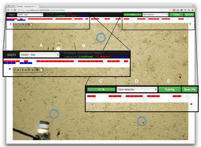
Figure 1. Screenshot of the DELPHI web interface. In the black top bar are the main navigation elements: on the left is a drop-down menu to select the transect within which laser points will be detected (A). Next to that, some information regarding the amount of laser point annotations and the detection performance are given (if available) (B). On the right, there is a visualization of the amount of annotations made (C), a selection box containing already trained detectors for other transects (D), as well as the button to train the detection system or start a detection (E). Directly below, a horizontal visualization of the complete transect is shown, spanning the whole width of the interface. Red rectangles stand for images where laser points were automatically detected, blue rectangles stand for images that have been annotated. The main part of the browser window is occupied by one transect image, in this case with three correctly detected LPs (highlighted for the figure with light blue circles). To the left/right of the image are arrows that allow to step to the previous/next image of the transect. In the top left part of the image are the buttons to zoom in and out of the image as well as move the image itself to the top/ bottom and left/right respectively to set the focus on the region of the image where laser points occur.

To moderate the data flow between the user interface and the C++ backend, an Apache web server is used (see Figure 2). This server runs PHP scripts to process data, e.g., to fetch all detections and send them to the GUI. The communication step is enabled through JSON RPC. For the communication with the C++ backend, the Apache server uses a Python DRMAA interface. Final detections ${\widehat{T}}^{(i,{\widehat{t}}^{(i)})}$ are stored in the file system while manual annotations T^(j) and confirmed detections are stored in the BIIGLE MySQL database.

FIGURE 2

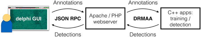
Figure 2. The detection framework. On the left is the field expert, interacting with the DELPHI GUI in a web browser. The annotations are transferred via JSON RPC to a web server. This server then starts the training process, which takes ca. 2 min. Afterwards (or in case an already trained detection system is applied), the web server schedules a detection process on the compute server. This makes the LP detection for a whole transect possible in <5 min. The field expert can poll for the results, which are transferred back to the DELPHI GUI through JSON RPC when the detection is completed. The web interface is then updated based on the results. A further iteration of LP annotation/correction with subsequent training and detection can follow if the detection result is seen as improvable.

Apart from the training and detection steps, which could in principle also be implemented in PHP and be run on the Apache server, DELPHI is runnable on any typical W/M/XAMP server.

4. Materials

To test the DELPHI approach, two image sets were evaluated. The first one is a transect taken in the Clarion-Clipperton fracture zone in the eastern Pacific Ocean (T1) (von Stackelberg and Beiersdorf, 1991). The second is a transect taken in the eastern Fram Strait (Arctic) at the HAUSGARTEN observatory (Bergmann et al., 2011) during Polarstern expedition ARK XX/1 (T2). The goal for T1 was to estimate the amount and size of poly-metallic nodules occurring on the seafloor (exploration scenario). The aim for T2 was to assess megafaunal densities and describe seafloor characteristics (detection scenario). Both image sets were captured with a towed camera rig (OFOS) that contains a downwardly facing camera. Because of the swell at the water surface, the camera altitude varies in both settings. The images thus show a rectangular area of the seafloor with varying pixel-to-centimeter ratio.

To allow for quantitative size measurements, three red laser points were projected on the seafloor in both transects. For T1, the OFOS was steered at a larger altitude, thus the color spectrum of the images (and the LPs) was shifted toward blueish/greenish colors. Here, the LP spatial layout consisted of two outer LPs with a distance of 20 cm that pointed straight down on the seafloor. The laser that created the LP between these two was attached with some angle to the OFOS and thus moved, relative to the outer two. This relative movement allows to compute the OFOS altitude.

For T2, the OFOS was towed closer to the seafloor and thus the images contained on average more red signal compared to T1. In this case, the LPs were all pointing straight down on the seafloor and arranged in a isosceles triangle with 50 cm side length. Figure 3 shows two image patches from T1 and T2 respectively that show the sub-region of one sample image where LPs occur. The highlighted parts show the mask M^(*) after 90 manual annotations to visualize the varying LP spatial layout. The Gaussian-like distributions of the position of the individual LPs for T2 occurs as a result of the pitch and roll of the camera rig and seafloor topography.

FIGURE 3

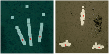
Figure 3. Examples for two different LP spatial layouts with detection masks (highlighted parts), corresponding to 90 annotated LPs each. The left part shows the spatial layout for T1, the right part for T2. Both cases show an example of a successful detection where the detected LP positions are given as red circles.

For both transects, manual annotations were available for more than 99% of the images in the transect. These annotations were used to compute classifier statistics (precision, recall, F-score) to evaluate the detection performance regarding the LP candidates detected by DELPHI. This performance evaluation was done iteratively with increasing training set size (N′ = 1, 2, 3, …, 10, 13, 16, …, 25, 27, 30). The manual annotation of one image with DELPHI requires about 10 s. The whole annotation process for the largest training set (N′ = 30) thus took ca. 5 min.

For comparison, we also applied to each of both transects alternative LP detection algorithms. These were based on a manually tuned color threshold and an explicitly defined model of the spatial layout of the LPs. Both alternative detections were defined by users in a time-consuming tuning process, including many corrections and feedback loops.

5. Results

Figure 4 contains the detection performance for T1 and T2. The detection performance rises at first with increasing training set size N′ but settles eventually. After 13 annotated images (i.e., 39 LP annotations or about 2 min effort), the detection performance lies ca. eight percent-points below (above) the average of the performances for larger training sets (i.e., N′ > 13). The average F-score after thirteen annotated images is 0.86 for T1 and 0.58 for T2.

FIGURE 4

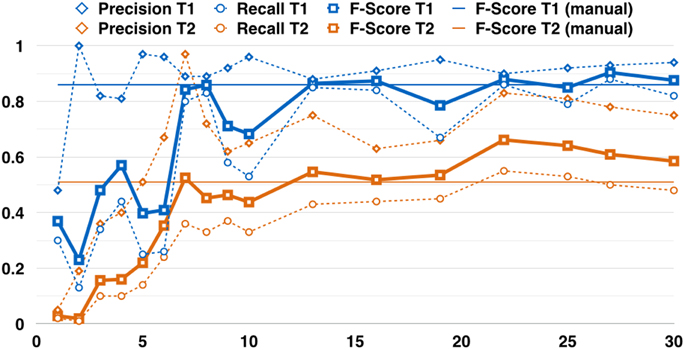
Figure 4. Two examples for the detection performance vs. the amount of images that were manually annotated (N_I). The blue curves (T1) are based on the Clarion Clipperton transect, the orange curves (T2) for the HAUSGARTEN transect. Note, that the performance does not chance a lot after ca. thirteen annotated images. This corresponds to one (two) % of the total amount of images in transect T1 (T2). The dashed curves indicate the precision (diamonds) and the recall (circles). The bold lines show the F-Score (squares). The thin straight lines indicate the detection performance for a manually tuned detection system for each individual transect (before DELPHI was established). These are horizontal lines as they represent the performance regarding the final tuned parameters for all images, rather than for a training set of increasing size.

The manually tuned detection system, that was used before DELPHI, resulted in an F-score of 0.86 for T1 and an F-Score of 0.51 for T2. This shows, that a major improvement regarding training time could be incorporated as well as a minor improvement regarding the detection performance.

6. Discussion

DELPHI was designed to detect LP spatial layouts with three LPs. In principle it could easily be extended to detect two or more than three LPs. The LP spatial layout part of the training and detection steps would have to be adapted. From the amount of annotations made in an image, the number of LPs per image would be determined automatically. Still, three LPs provide usually enough information for quantification of the image content. More LPs are useful in areas of higher structural complexity and from where thus finer-scale information is required.

As stated in the introduction, the LPs can become practically invisible to the human eye, e.g., when the altitude becomes too large. In those cases, a pre-processing of the images can be useful that normalizes the color spectrum of the whole image and thus makes the LPs perceivable. Possible pre-processings are described in Bazeille et al. (2006); Schoening et al. (2012a) but were so far not incorporated in DELPHI. Each pre-processing takes time and would thus slow down the detection process.

7. Conclusion

In this paper, DELPHI was presented, the first web-based, adaptively learning laser point detection for benthic images. It was designed to learn different laser point spatial layouts and laser point colors from a small set of manual annotations. By applying it to two real-world scenarios, a major improvement regarding the training effort and a minor improvement regarding the detection performance could be achieved. DELPHI thus proved to be as effective as a time-consuming individual tuning of detection parameters while further being more efficient as well.

7.1. Accessing DELPHI

A test login for DELPHI is available at https://ani.cebitec.uni-bielefeld.de/olymp/pan/delphi with the login name “test” and password “test.” A small transect (70 images) from the Hausgarten observatory can be annotated and the detection system be trained and applied. The trained detectors are automatically deleted after 1 day.

Conflict of Interest Statement

The authors declare that the research was conducted in the absence of any commercial or financial relationships that could be construed as a potential conflict of interest.

Acknowledgments

We thank the BGR for providing the images used to evaluate the detection process. This work was funded by the German Federal Ministry for Economics and Technology (BMWI, FKZ 03SX344A). Part of the footage used in this paper was generated during expeditions of the research icebreaker Polarstern to the HAUSGARTEN observatory. This publication is Eprint ID 34764 of the Alfred-Wegener-Institut Helmholtz-Zentrum für Polar- und Meeresforschung.

References

Bazeille, S., Quidu, I., Jaulin, L., and Malkasse, J.-P. (2006). “Automatic underwater image pre-processing,” in Proceedings of CMM'06 (Brest).

Google Scholar

Bergmann, M., Langwald, N., Ontrup, J., Soltwedel, T., Schewe, I., Klages, M., et al. (2011). Megafaunal assemblages from two shelf stations west of Svalbard. Marine Biol. Res. 7, 525–539. doi: 10.1080/17451000.2010.535834

CrossRef Full Text | Google Scholar

Bradski, G. (2000). Opencv. Dr. Dobb's Journal of Software Tools.

Lüdtke, A., Jerosch, K., Herzog, O., and Schlüter, M. (2012). Development of a machine learning technique for automatic analysis of seafloor image data: Case example, pogonophora coverage at mud volcanoes. Comput. Geosci. 39, 120–128. doi: 10.1016/j.cageo.2011.06.020

CrossRef Full Text | Google Scholar

MacLeod, N., and Culverhouse, P. (2010). Time to automate identification. Nature 467, 154–155. doi: 10.1038/467154a

PubMed Abstract | Full Text | CrossRef Full Text | Google Scholar

Ontrup, J., Ehnert, N., Bergmann, M., Nattkemper, T. (2009). “BIIGLE - Web 2.0 enabled labelling and exploring of images from the Arctic deep-sea observatory HAUSGARTEN,” in OCEANS 2009, (Bremen), 1–7.

Google Scholar

Pilgrim, D., Parry, D., Jones, M., and Kendall, M. (2000). Rov image scaling with laser spot patterns. Underwater Technol. 24, 93–103. doi: 10.3723/175605400783259684

CrossRef Full Text | Google Scholar

Purser, A., Bergmann, M., Lundälv, T., Ontrup, J., and Nattkemper, T. W. (2009). Use of machine-learning algorithms for the automated detection of cold-water coral habitats - a pilot study. Marine Ecol. Prog. Ser. 397, 241–251. doi: 10.3354/meps08154

CrossRef Full Text | Google Scholar

Schoening, T., Bergmann, M., Ontrup, J., Taylor, J., Dannheim, J., Gutt, J., et al. (2012a). Semi-automated image analysis for the assessment of megafaunal densities at the arctic deep-sea observatory HAUSGARTEN. PLoS ONE 7:e38179. doi: 10.1371/journal.pone.0038179

CrossRef Full Text | Google Scholar

Schoening, T., Kuhn, T., and Nattkemper, T. W. (2012b). “Estimation of poly-metallic nodule coverage in benthic images,” In Proceeding of the 41st Conference of the Underwater Mining Institute (UMI) (Shanghai).

Schoening, T., Steinbrink, B., Brün, D., Kuhn, T., and Nattkemper, T. W. (2013). “Ultra-fast segmentation and quantification of poly-metallic nodule coverage in high-resolution digital images,” in Proceedings of the UMI 2013 (Rio de Janeiro).

Google Scholar

von Stackelberg, U. and Beiersdorf, H. (1991). The formation of manganese nodules between the Clarion and Clipperton fracture zones southeast of Hawaii. Marine Geol. 98, 411–423.

Google Scholar

Williams, S. B., Pizarro, O., Jakuba, M., and Barrett, N. (2010). “AUV benthic habitat mapping in south eastern Tasmania,” in Field and Service Robotics, (Berlin; Heidelberg: Springer), 275–284.

Google Scholar