Productivity changes in the Mediterranean Sea for the twenty-first century in response to changes in the regional atmospheric forcing

Introduction

The Mediterranean Sea has been described as a hot-spot for climate change (Giorgi, 2006) because of a number of reasons. Firstly, it is located in a temperate region which is expected to become warmer and drier in the nearby future (IPCC, 2013). Secondly it is a semi-enclosed basin being, thereby, strongly influenced by continental conditions. Thirdly, it hosts a very large human population that exerts a considerable influence on the marine ecosystems' conditions (e.g., Macías et al., 2014a).

Climatic and anthropogenic forcings will combine in the future in uncertain ways and will potentially create a wide range of pressures on the Mediterranean Sea ecosystems. The only way to try to assess expected future consequences is through scenario generation using a set of numerical interconnected models (Najjar et al., 2000; Uncles, 2003). Three elements should, at least, be included in the scenario generation process, the atmosphere, the ocean, and the socio-economic activity. With such interconnected models, attribution exercises could be performed by isolating sources of variability and assessing potential changes on the variables of interest by the individual forcing factors (e.g., atmospheric conditions, river discharges, or human activities). In the present contribution, our aim is to evaluate the direct effects of alterations in atmospheric forcing due to climate change on the biogeochemical conditions of the Mediterranean Sea.

Numerical models have been mostly used to study changes in physical properties of the Mediterranean basin under different future scenarios. For example, the future evolution of the Mediterranean Thermohaline Circulation (MTHC) has been assessed in a number of works (e.g., Thorpe and Bigg, 2000; Somot et al., 2006) while water and heat fluxes evolution throughout the basin have been investigated under different emission scenarios (e.g., Christensen et al., 2007; Dubois et al., 2012). A review of the studies dealing with Mediterranean climate projections can be found in Planton et al. (2012).

However, assessments of potential changes on Mediterranean biological production characteristics in future scenarios are much less common. One of the few works evaluating basing wide changes on trophic regimes in climate scenarios was presented by Lazzari et al. (2014) which, however, considered just one single emission scenario (A1B) from the outdated Coupled Model Intercomparison Project Phase 3 (CMIP3) and used a time-slice approach which has some disadvantages compared to transient simulations (e.g., Gualdi et al., 2013). Also, Herrmann et al. (2014) made an assessment of the potential impacts of climate change on the NW Mediterranean Sea pelagic ecosystems. Besides these two works, to the best of our knowledge little more has been done regarding biogeochemical consequences of climatic scenarios in the Mediterranean Sea.

Biological productivity in the Mediterranean basin is typically dominated by a winter-spring bloom happening in some restricted areas (e.g., D'Ortenzio and Ribera d'Alcala, 2009) controlled by vertical mixing during winter time (Siokou-Frangou et al., 2010). Production associated to upwelling events is much lower and only associated to specific regions such as the NW Alboran Sea (e.g., Garcia-Gorriz and Carr, 2001). Henceforth, to correctly reproduce production levels and distribution with a numerical model, vertical stratification characteristics of the basin should be reasonably simulated.

Here we will use an ocean model already proven to provide a reasonable representation of past and present hydrodynamic and biogeochemical conditions of the Mediterranean basin (Macías et al., 2013, 2014a,c) to explore a set of future scenarios for the basin. This ocean model is forced at the surface with atmospheric variables provided by a regional circulation model (RCM) forced at the boundaries with different global climate models (GCMs) included in the Coupled Model Intercomparison Project Phase 5 CMIP5 exercise. Different emission scenarios for each GCM are considered, including the worst-case scenario (rcp8.5 or business as usual case) where emissions continue to grow throughout the entire twenty-first century and an intermediate, more desirable case (rcp4.5) where emissions peak ~2040 and decline afterwards. The different model runs are performed continuously from 2013 to 2100 so the transient evolution of the system is fully considered.

For the present contribution no year-to-year change in freshwater flow or nutrient concentrations in riverine waters is contemplated. This way the direct effect of changing atmospheric conditions on the marine ecosystem could be detected and isolated from the anthropogenic effects mainly happening by the modifications of rivers conditions.

The ocean model and atmospheric forcing used are exposed in Section Materials and Methods. Main results are presented in Section Results while conclusions could be found in Section Discussion.

Materials and Methods

Mediterranean Ocean Model

The 3-D General Estuarine Transport Model (GETM) was used to simulate the hydrodynamics in the Mediterranean Sea. GETM solves the three-dimensional hydrostatic equations of motion applying the Boussinesq approximation and the eddy viscosity assumption (Burchard and Bolding, 2002). A detailed description of the GETM equations could be found in Stips et al. (2004) and at http://www.getm.eu.

The configuration of the Mediterranean Sea (Figure 1) has a horizontal resolution of 5′ × 5′ and includes 25 vertical sigma-layers. A third-order Total Variation Diminishing (TVD) numerical scheme is used as recommended by Burchard et al. (2006). ETOPO1 (http://www.ngdc.noaa.gov/mgg/global/) was used to build the bathymetric grid by averaging depth levels to the corresponding horizontal resolution of the model grid. To avoid truncation errors over steep topographies (e.g., Haney, 1991) smoothing was applied before starting the simulations to the bathymetric grid by using the method proposed for ROMS (http://www.romsagrif.org). This method allows to prescribe the tolerance in the difference of depths for adjacent cells. The salinity and temperature climatologies required at the start of the model integration were obtained from the Mediterranean Data Archeology and Rescue-MEDAR/MEDATLAS database (http://www.ifremer.fr/medar/) while biogeochemical initial and boundary conditions were computed from the World Ocean Atlas database (www.nodc.noaa.gov/OC5/indprod.html). All model runs described below started with exactly the same initial conditions.

FIGURE 1

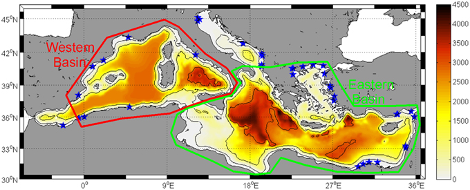
Figure 1. Model domain with bathymetry (background color). Blue stars indicate the position of the river mouths included in the model. The red and green polygons indicate the areas considered as Western and Eastern basins in this work.

Boundary conditions at the western entrance of the Strait of Gibraltar were also computed from the same MEDAR/MEDATLAS dataset imposing monthly climatological vertically-explicit values of salinity. Sea surface temperature at the western entrance of the Strait were extracted from the nearest node of the driven GCM for each simulation (see below) while the rest of the water column temperature was not changed. This configuration did not fundamentally modify the conditions of the Atlantic inflow during the simulations, which allows to better isolate the effects of a changing atmospheric forcing as explained below. No horizontal currents were imposed at the open boundary. With this boundary configuration the circulation through the Strait is stablished by the internally-adjusted baroclinic balance provoked mainly by the deep-water formation within the basin (Macias et al., under review). Although the magnitude of the interchanged flow and horizontal velocities in Gibraltar are in agreement with observations (not shown) the circulation pattern within the Alboran Sea is not in concordance with measurements as the eastern gyre is typically weaker than expected (Macias et al., under review).

The GETM configuration for the Mediterranean Sea is forced at surface every 6 h by the following atmospheric variables, wind velocity at 10 m (U10 and V10), air temperature at 2 m (t2), specific humidity (sh), cloud cover (tcc), and sea level pressure (SLP) provided by the different realizations of the atmospheric model described in the next section. Bulk formulae are used to calculate the corresponding relevant heat, mass, and momentum fluxes between atmosphere and ocean (Macías et al., 2013).

Regional Climate Model

The ocean model described above is forced at the surface with the outputs provided by the Cosmos-CLM (http://www.clm-community.eu/) RCM implemented within the EuroCORDEX initiative (http://www.euro-cordex.net/). This RCM is forced at the boundaries with conditions provided by two global circulation models (GCMs) included in the CMIP5 exercise (Table 1), MPI and EcEarth (http://cmip-pcmdi.llnl.gov/cmip5/). For each GCM two emission scenarios as defined by IPCC are considered; rcp4.5 and rcp8.5 (Meinshausen et al., 2011). Hence a total of four member ensemble runs are analyzed in this work.

TABLE 1

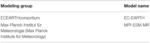
Table 1. Institutes/modeling groups providing the atmospheric model data used in the present contribution.

Atmospheric variables provided by the RCM realizations induce an underestimation of simulated SST for the present-day (Macias et al., under review) so a bias-correction of the most relevant variables (air temperature, cloud cover, and wind intensity) has been performed as proposed by Piani et al. (2010). The basic principle of this technique is to find a transfer function that allows matching the cumulative distribution functions (CDFs) of modeled and observed data (Dosio and Paruolo, 2011; Dosio et al., 2012). We have employed as observations the reanalysis data contained in the ECMWF ERAin dataset. Spatially-averaged values of the observed and model variables over the entire Mediterranean Sea basin were used, so no spatially explicit correction was applied. By doing so, the initial conditions of the scenario runs (forced with the RCM variables) compare quite well with the end of hindcast simulations forced with ERAin reanalysis (Dee et al., 2011) as shown in Figures 2, 6 below. Also seasonality and spatial distribution of SST compare well with observed satellite patterns for the recent decades (1989–2005) as shown by Macias et al. (under review).

FIGURE 2

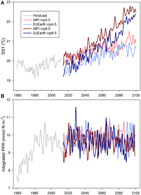
Figure 2. Time series of mean (basin averaged) (A) sea surface temperature (SST) and (B) surface (50 m) primary production rate (PPR) for the hindcast (gray line) and the different simulation scenarios (color lines).

Rivers′ Conditions

The present configuration of the ocean model includes 37 rivers discharging along the Mediterranean coast (blue stars in Figure 1). The corresponding river discharges were derived from the Global River Data Center (GRDC, Germany) database. Nutrient content (nitrate and phosphate) of freshwater runoff were obtained from Ludwig et al. (2009). For the full extent of the performed scenario simulations (2013–2100) river fluxes and nutrient loads where kept constant and equal to their seasonal climatological values during the years 1985–2000.

Results

Basin-wide averaged annual sea surface temperature (SST) and primary productivity rate integrated in the upper 50 m (PPR) are shown in Figure 2 for the hindcast run (1960–2012) and for the different scenarios runs (2014–2100). The hindcast run is described in Macías et al. (2013, 2014a) and has been included in the figures to allow comparison with the different future scenarios. As expected, SST continuously increase in the different scenario runs with the two rcp4.5 runs (light colored lines in Figure 2A) showing a mean warming of ~1°C by 2100 (i.e., a warming rate of ~0.12°C/decade for MPI and ~0.14°C/decade for EcEarth) and the two rcp8.5 runs (dark colored lines in Figure 2A) indicating a warming of ~2.7°C by 2100 (~0.32°C/decade for both MPI and EcEarth). MPI-driven simulations (red lines in Figure 2A) are typically warmer than the EcEarth runs (blue lines in Figure 2A) for the two different scenarios considered.

PPR time series are quite constant during the different scenario runs (colored lines in Figure 2B) showing no significant trend but quite a strong interannual variability. On the contrary, the hindcast simulation (gray line in Figure 2B) shows the transition from low to high PPR described and commented by Macías et al. (2014a) linked with the rivers′ flow and nutrients loads changes. It is also noteworthy the relative good agreement of the mean SST and PPR at the end of the hindcast (gray lines in Figure 2) and the initial years of the scenario runs (colored lines in Figure 2), even if in SST in some runs (especially those forced by EcEarth) present some small cold bias (~0.4°C).

Spatial maps of SST and PPR anomalies (mean from 2095 to 2099 minus mean from 2015 to 2019) for the different scenario runs are shown in Figure 3. For SST there is no consistent spatial structure in the different runs and only the stronger warming in rcp8.5 (Figures 3C,D) could be clearly observed when compared with the rcp4.5 runs (Figures 3A,B). For PPR, on the contrary, a consistent pattern could be observed in all scenario runs as the western basin tends to show negative PPR anomalies values (i.e., more oligotrophy) while the eastern basin consistently show positive PPR anomalies (i.e., more eutrophic). The consistency of this PPR anomaly pattern is further confirmed by the maps in Figure 4 where the ensemble mean (i.e., the mean value of all four scenario runs) is shown in Figure 4A and the ensemble standard deviation in Figure 4B. The mean PPR anomaly map show the already described west-east gradient (negative to positive) while the standard deviation map indicate a very low inter-runs variability except for the Alboran Sea region.

FIGURE 3

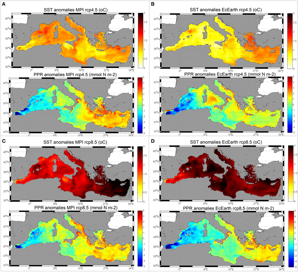
Figure 3. Spatial maps of SST and PPR anomalies (mean from 2095 to 2099 minus 2015–2019) for the different scenario runs. (A) MPI rcp45.5, (B) EcEarth rcp4.5, (C) MPI rcp8.5, (D) EcEarth rcp8.5.

FIGURE 4

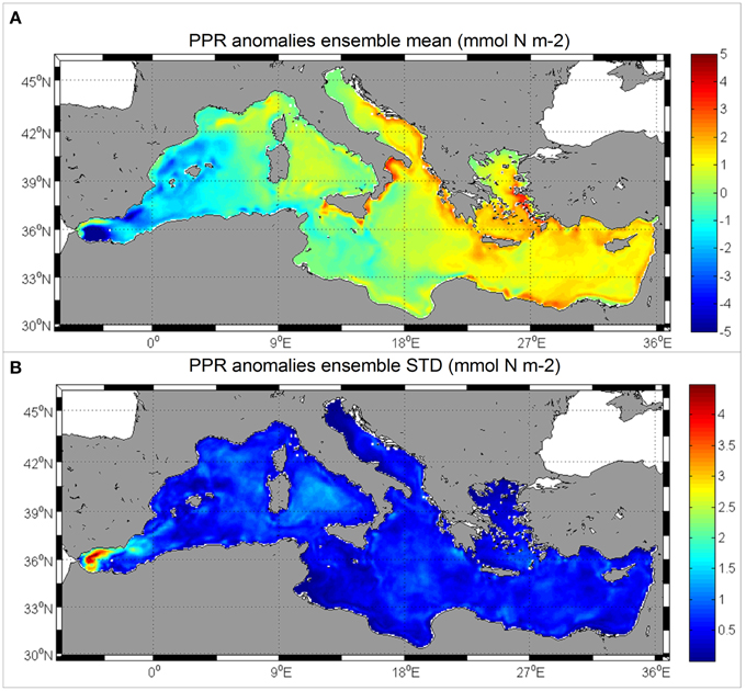
Figure 4. (A) Mean PPR anomalies (2095–2099 minus 2015–2019) for all the simulations run under the different scenarios/models (ENSEMBLE mean). (B) Standard deviation of the PPR anomalies between the different scenarios/models runs.

In order to understand further the potential reasons for the spatial distribution of PPR anomalies, the seasonal SST and PPR cycles for the beginning of the scenario runs (2015–2019) (gray line in Figure 5) are compared with those for the end of the runs (2095–2099) (color lines in Figure 5). For SST (Figure 5A) there are no evident seasonal differences and each model has a quite similar season-to-season anomaly along the entire year. As seen in Figure 2A, in the MPI-driven simulations the warming anomaly is consistently larger than in the EcEarth for the two considered rcp.

FIGURE 5

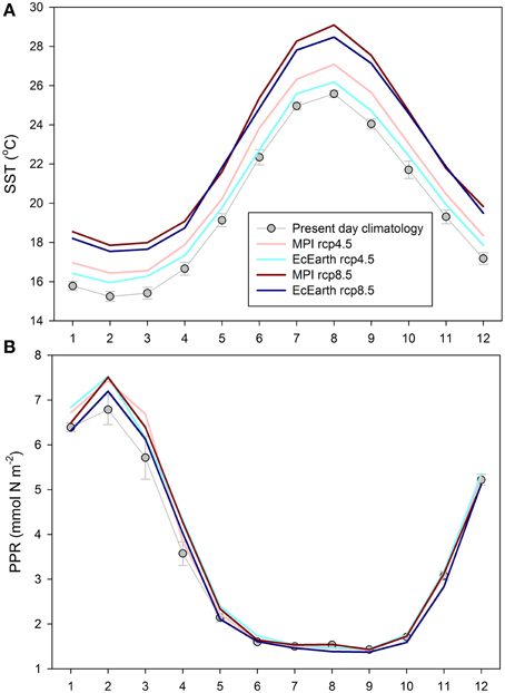
Figure 5. Climatological cycles of (A) SST and (B) PPR at the beginning of the different runs (gray lines, 2015–2019) and at the end (2095–2099) of each scenario run. The errors bars indicate the dispersion between model runs for the beginning simulation period.

For PPR, however, only significant deviations (positive) are observed for the end of all scenario runs during the winter/spring months (January–April) as shown in Figure 5B. PPR values are quite similar in all model runs except for EcEarth rcp8.5 which is consistently lower than the other three model runs. This is clearly indicating that in the future scenarios the winter/spring blooms are larger than in the present day conditions. As such blooms are typically linked to winter mixing events, it would be advisable to analyze the forecasted surface density changes for the different scenarios.

Surface density is going to be affected by the warmer SST in the future but also by potential changes in surface salinity. Basin-wide averaged annual surface salinity (SSS) are shown in Figure 6A for the hindcast (gray lines) and for the different scenario runs (color lines).

FIGURE 6

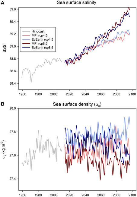
Figure 6. Time series of mean (basin averaged) (A) sea surface salinity (SSS) and (B) surface density (σ₀) for the hindcast (gray line) and the different simulation scenarios (color lines).

As happened with SST, SSS increases in all scenarios with a larger increase in rcp8.5 (~0.09/decade) than in rcp4.5 (~0.05/decade). During the hindcast run (gray line in Figure 6A) the salinity also increased but at a much smaller rate (~0.019/decade). If both SST and SSS are combined to compute the surface density averaged over the entire basin (Figure 6B) it could be seen that it did not significantly change in the different scenarios. This is due to the opposite effect of warming (decrease density) and salinization (increase density) compensating each other along the simulations.

Plotting the surface density anomaly maps between the end (2095–2099) and the beginning (2015–2019) of the different simulations (Figures 7A–D) a familiar pattern emerges, with the western basin showing surface density reduction (i.e., increased vertical stratification) while the eastern basin shows surface density increase (i.e., reduced vertical stratification assuming constant deep density). The ensemble average map of mean surface density anomaly (Figure 7E) does, indeed, resemble the one for PPR anomalies shown in Figure 4A.

FIGURE 7

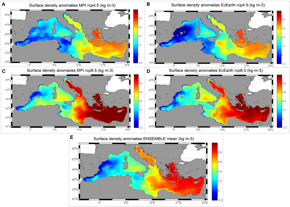
Figure 7. (A–D) Surface density anomalies (2095–2099 minus 2015–2019) for the different simulations runs. (E) Mean surface density anomalies in all scenario runs (ENSEMBLE mean).

The similarities between density and PPR anomalies are further shown by the scatter plot in Figure 8. Here, it is clear that regions with a negative density anomaly (i.e., where surface water becomes lighter) correspond with a negative PPR anomaly (oligotrophy) while regions where surface water becomes denser correspond with positive PPR anomalies. The linear fit of all simulations together is indicated in Figure 8A by the green line and has a correlation coefficient of 0.48. The same linear fitting could be obtained for each of the individual runs (Figures 8B–E) all with significant correlations ranging from 0.47 to 0.67. In those individual scatters it becomes clear that the western basin (as defined by the red polygon in Figure 1) is typically on the lower left corner of the plots (crosses in Figures 8B–E) while the eastern basin (green polygon in Figure 1) occupies the upper right corner of the plots (circles in Figures 8B–E).

FIGURE 8

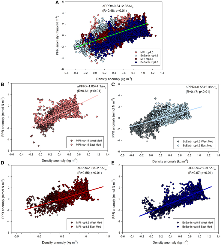
Figure 8. Scatter plot of surface density anomalies vs. PPR anomalies in the different runs. (A) All scenario runs, (B) MPI rcp4.5, (C) EcEarth rcp4.5, (D) MPI rcp8.5, (E) EcEarth rcp8.5.

Discussion

As expected, simulated SST during the different scenario runs show a continuous warming of the surface Mediterranean basin in concordance with previous works (e.g., Somot et al., 2006; Lazzari et al., 2014). In the time evolution of SST during the next century (Figure 2A) there is only a monotonic trend to be observed in contrast with the existence of a multidecadal oscillation (Schlesinger and Ramankutty, 1994) during the hindcast period (Macías et al., 2013). The lack of the correct natural variability in current generation climate models have already been pointed out elsewhere (Fyfe et al., 2013; Kavvada et al., 2013) and have been also related with the overestimation of simulated global surface temperature during the last 10 years (e.g., Guemas et al., 2013; Macías et al., 2014c). However, the warming trend is very consistent in all simulation runs and the final total warming in the different scenarios are in line with the most probable trajectory of the system (e.g., Somot et al., 2008; Gualdi et al., 2013).

It is also important the fact that by applying bias correction techniques to the atmospheric variables, we have been able to almost level the final SST conditions during the hindcast runs (forced by ERAin reanalysis) and the initial years of the scenarios. Without applying bias correction, simulated SST during the period 1989–2005 was between −1.4°C and −1.8°C for MPI and EcEarth respectively (Macias et al., under review) when compared with the SST obtained with ERAin forcing for the same period in agreement with previous model/reanalysis comparisons for the recent decades (e.g., Dell'Aquila et al., 2012). In the runs presented here, this cold bias is reduced (with respect to the final years of the hindcast run) to ~−0.1°C for MPI and ~−0.4°C and EcEarth. This provides a more suitable starting point for the scenario simulations and allows to analyze the complete transient evolution of the system from the actual conditions, avoiding the need of using a time-slice approach which has many associated problems (Gualdi et al., 2013). The correct representation of the actual SST values imply that the density structure is, also, better simulated in the models and, hence, the strength of vertical mixing (e.g., Vichi et al., 2003; Steinacher et al., 2010). This is one of the reasons why present-day PPR mean levels are also correctly simulated in the different scenario runs (Figure 2B).

Regarding this PPR, the four scenario runs presented in this work clearly indicate that changes in atmospheric forcing alone will not significantly alter its mean integrated value in the Mediterranean basin (Figure 2B). Even if winter PPR values are shown to be larger in the future scenarios (Figure 5B) annual mean PPR is not significantly different (t-student test, 99% probability) at the beginning and the end in any of the performed simulations. This is in consistency with the previously described influence of riverine water quality (nutrients concentrations and relative abundance) on the global productivity of the basin (Macías et al., 2014a). In this previous work, it has been described the causal link between freshwater quality changes derived from European legislation and the alteration of marine productivity in the whole Mediterranean basin extending from primary producers to high trophic levels. The results obtained in the present ensemble of simulations with a quasi-constant integrated PPR levels linked with non-changing rivers conditions are an additional proof of the importance of riverine discharges for the overall productivity of the basin.

However, the seasonal cycle of PPR is simulated to change in the future scenarios, with enhanced winter/spring blooms compared with present-day conditions. The rest of the seasonal PPR cycle seems not to change significantly with mean levels compared to present day values (Figure 5B). As recently shown by Macías et al. (2014c), a substantial fraction of the basin PPR happen in subsurface chlorophyll accumulations (DCMs) especially during the stratified period of the year. To further understand the changes in integrated PPR simulated for the different scenarios, the mean monthly position (depth) and spread (% of the open sea basin) of the DCMs are compared in Figure 10. The present day conditions (Figure 10A) shows the already described pattern with more abundant and deep DCMs during the summer months, being shallower and less common in winter/fall. The anomalies (values at the end of the simulation—values at the beginning) shown in Figures 10B–E indicate that larger differences are typically simulated to occur in winter/spring when DCMs tend to be shallower but more common in the open Mediterranean by the end of the century. During summer the differences are typically lower in the different simulated scenarios. On average, there is a small reduction of the mean depth of the DCMs in the future scenarios (0.3–2.1 m, mean = 1.2 m) and a larger percentage of the open sea basin showing these structures (0.3–3.8%, mean = 1.8%).

The generalized increase in winter/spring blooms in the scenarios (Figure 5B) is most likely linked to vertical density changes created by the combination of warming and salinization. As shown for the present day conditions, production during these months happens in a wide layer on the surface ocean (Macías et al., 2014c) with less prominent vertical structures, so surface changes could be considered a good measure of total water column alterations. More intense winter/spring blooms could have consequences for energy and biomass transfer up the food web as, for example, winter-spawning species (e.g., sardine) will have a competitive advantage in terms of food availability with respect to summer-spawning species (e.g., anchovy) (Ruiz et al., 2013; Macías et al., 2014b).

The most typical consequence of a warmer earth future for marine ecosystems is the increase in the surface water temperature which, consequently, increases vertical stratification (Manabe et al., 1991; Sarmiento et al., 1998; Bopp et al., 2001). This increase in water column stability makes vertical mixing more difficult and, thus, surface primary production is expected to reduce (e.g., Behrenfeld et al., 2006) leading to a reduction of the biologically-mediated carbon export to the deep ocean. This represents a positive feedback mechanism for global warming (Sarmiento et al., 1998; Bopp et al., 2001; Schmittner, 2005).

As recently pointed out by Marañón et al. (2014), stratification changes are more important for future PPR in the global ocean than the direct effect to warming on biological rates. We have, thus, computed the changes in mean vertical stratification (defined as the density differences between surface and 50 m) and compare them with the PPR anomalies in Figure 9. As it could be seen, regions where vertical stratification decreases or remain unchanged, typically show positive PPR anomalies while where vertical stratification increases, PPR decreases.

FIGURE 9

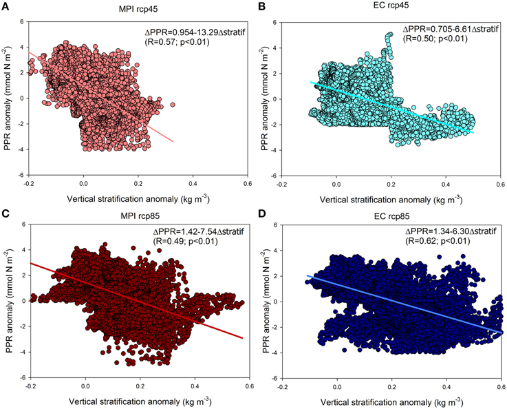
Figure 9. Scatter plot of vertical stratification (density at 50 m—surface density) anomalies vs. PPR anomalies in the different runs. (A) MPI rcp4.5, (B) EcEarth rcp4.5, (C) MPI rcp8.5, (D) EcEarth rcp8.5.

FIGURE 10

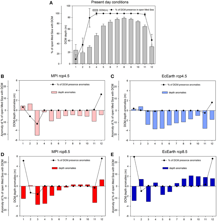
Figure 10. (A) Present day (2015–2019) mean DCM depth (bars) and % of the basin showing the presence of DCMs (lines). (B–E) Anomalies (future-present) values of the DCMs depth (bars) and areal coverage (lines) for the four scenarios.

For the Mediterranean Sea, being an evaporative basin, it is necessary to consider also the potential changes in salinity to evaluate the surface density anomalies. As shown by Figure 6A, surface salinity is simulated to increase in all scenarios with a variable rate depending on the emission scenario considered. Salinity in Mediterranean basin-wide models is a quite difficult variable to simulate as its temporal evolution depends very much on the model set-up, including bathymetric details and, particularly, the Gibraltar Strait configuration (e.g., Naranjo et al., 2014). If the simulated water interchange through the Strait is not similar to its real value, there could be a salt accumulation (or loss) from the initial conditions that will affect the temporal evolution of this variable. However, as shown by the hindcast simulation (gray line in Figure 6A) for this specific model set-up it seems that salinity (at least surface values) are quite stable with a slight salinification trend as already described from field data (e.g., Borghini et al., 2014). Henceforth, it is quite reasonable to assume that the observed salinity trends in the scenario runs are driven by the changing atmospheric conditions (especially if we consider that freshwater inputs are not changing throughout the simulations).

The salinity anomaly provokes a very clear pattern of surface density changes, with the region closer to the Strait of Gibraltar showing a reduction of surface density (i.e., warming being more relevant) while in the regions further away from the Strait surface density tends to increase (i.e., salinization is more important) (Figure 7). The extent of the region with positive or negative surface anomalies change in the different emission scenarios considered. For rcp4.5 ~ 33% of the basin is simulated to present negative density anomalies (34% for MPI and 31% for EcEarth) while for rcp8.5 this percentage reduces to ~ 1.4% (1.3% for MPI and 1.5% for EcEarth). This numbers indicate that the effect of warming is relatively (compared to salinization) more important in rcp4.5 than in rcp8.5 where the increase of salinity is much acute and generalized.

Associated to these surface density changes (and vertical mixing strength) there is a very consistent PPR anomaly distribution as shown by Figure 4A. A clear dipole could be observed with a generalized reduction of surface productivity in the areas affected by the surface density decrease while in regions where surface density enhances, PPR also do increase. A productivity increase in the eastern basin in future scenarios has been previously linked to increase population and, hence, nutrient inputs in this region (Lazzari et al., 2014) although this is not the case in our simulations as rivers conditions are kept unchanged. Our results are somehow in line with the recent findings by Chust et al. (2014), who found that while the general trend in the overall ocean is to decrease PPR with an increase of the vertical stratification in future scenarios, there are some regional exception where models predict an increase on surface production level associated with a warmer climate.

The exact extension of the region affected by the fresher waters coming from the Atlantic Ocean is going to depend on the salinity of those waters. In our simulations we have maintained the salinity unchanged in the boundary because of its complex past behavior (e.g., Curry et al., 2003) and the large uncertainty associated to its future evolution. Atlantic waters salinity will be affected by the same evaporative processes described for the Mediterranean here but also by the melting of ice sheet from the poles (Stroeve et al., 2012). How this two opposed process will alter future salinity is highly uncertain. If Atlantic waters salinity decreases, the oligotrophic regions shown in our scenarios will, likely, be enhanced. If, on the contrary, Atlantic surface salinity increases, the oligotrophic region in the Mediterranean should be expected to be smaller. The large importance of the Atlantic inflow on the future state of the Mediterranean biological production is also in agreement with its described significance for the future evolution of mass and heat fluxes (Adloff et al., 2015).

Finally, in the polygons shown in Figure 1 separating the scatter data presented in Figure 8 there are two regions excluded, the Adriatic and the Alboran Sea. The Adriatic Sea have been omitted because it has been shown that the used model could not correctly reproduce the present-day biogeochemical conditions of this sub-basin (Macías et al., 2014c) so it does not make sense to evaluate changes in the scenarios. On the other hand, the Alboran Sea has been excluded since is situated just on the boundary of the model and because there primary production characteristics has been shown to strongly depend on a number of complex interacting hydrological processes (Sarhan et al., 2000; Macías et al., 2007; Ruiz et al., 2013) specially, on the strength of the Atlantic Jet (AJ) (e.g., Oguz et al., 2014).

In conclusion, even if the proposed scenarios are not very realistic (because of the assumed constant river outflow) they could be considered useful in two different senses. Firstly, they allow to isolate the impact of direct atmospheric forcing on the surface layer of the Mediterranean Sea and with no direct anthropogenic interaction. And secondly, this ensemble of simulations could be considered as a baseline reference in order to evaluate more complex scenarios including both changes in freshwater fluxes and alteration of the chemical composition of riverine waters driven by socio-economic changes. Such complex scenarios are being currently evaluated within our group and will be presented in future associated works. Additionally, the effect of climatic changes on community composition and/or physiological adaptations are important topic for future endeavors trying to understand potential changes on Mediterranean Sea ecosystems.

Author Contributions

DM, AS, and EG jointly debated the new hypothesis, discussed the results and contributed to the manuscript. DM, EG, and AS developed the coupled models and designed the simulations. DM, AS, and EG performed the analyses and wrote the paper.

Conflict of Interest Statement

The authors declare that the research was conducted in the absence of any commercial or financial relationships that could be construed as a potential conflict of interest.

Acknowledgments

A. Dosio facilitated the atmospheric model runs to force the ocean model from the EuroCORDEX initiative database (http://www.euro-cordex.net/). We acknowledge the World Climate Research Programme's Working Group on Coupled Modeling, which is responsible for CMIP, and we thank the climate modeling groups (listed in Table 1 of this paper) for producing and making available their model output. For CMIP the U.S. Department of Energy's Program for Climate Model Diagnosis and Intercomparison provides coordinating support and led development of software infrastructure in partnership with the Global Organization for Earth System Science Portals.

References

Adloff, F., Somot, S., Sevault, F., Jorda, G., Aznar, R., Deque, M., et al. (2015). Mediterranean Sea response to climate change in an ensemble of twenty first century scenarios. Clim. Dyn. 2507, 1–28. doi: 10.1007/s00382-015-2507-3

CrossRef Full Text | Google Scholar

Behrenfeld, M. J., O'Malley, R. T., Siegel, D. A., McClain, C. R., Sarmiento, J. L., Feldman, G. C., et al. (2006). Climate-driven trends in contemporary ocean productivity. Nature 444, 752–755. doi: 10.1038/nature05317

PubMed Abstract | CrossRef Full Text | Google Scholar

Bopp, L., Monfray, P., Aumont, O., Dufresne, J. L., Le Treut, H., Madec, G., et al. (2001). Potential impact of climate change on marine export production. Glob. Biochem. Cycles 15, 81–99. doi: 10.1029/1999GB001256

CrossRef Full Text | Google Scholar

Borghini, M., Bryden, H., Schroeder, K., Sparnocchia, S., and Vetrano, A. (2014). The Mediterranean is getting saltier. Ocean Sci. Discuss. 11, 735–752. doi: 10.5194/osd-11-735-2014

CrossRef Full Text | Google Scholar

Burchard, H., and Bolding, K. (2002). GETM, a General Estuarine Transport Model in Scientific Documentation. Technical report, European Commission, Ispra, Italy.

Burchard, H., Bolding, K., Kuhn, W., Meister, A., Neumann, T., and Umlauf, L. (2006). Description of a flexible and extendable physical–biogeochemical model system for the water column. J. Mar. Syst. 61, 180–211. doi: 10.1016/j.jmarsys.2005.04.011

CrossRef Full Text | Google Scholar

Christensen, J. H., Carter, T. R., Rummukainen, M., and Amanatidis, G. (2007). Evaluating the performance and utility of regional climate models: the PRUDENCE project. Clim. Chang. 81, 1–6. doi: 10.1007/s10584-006-9211-6

CrossRef Full Text | Google Scholar

Chust, G., Allen, J. I., Bopp, L., Schrum, C., Holt, J., Tsiaras, K., et al. (2014). Biomass changes and trophic amplification of plankton in a warmer ocean. Glob. Chang. Biol. 20, 2124–2139. doi: 10.1111/gcb.12562

PubMed Abstract | CrossRef Full Text | Google Scholar

Curry, C., Dickson, B., and Yashayaev, V. (2003). A change in the freswater balance of the Atlantic Ocean over the past four decades. Nature 426, 826–829. doi: 10.1038/nature02206

PubMed Abstract | CrossRef Full Text | Google Scholar

Dee, D. P., Uppala, S. M., Simmons, A. J., Berrisford, P., Poli, P., Kobayashi, S., et al. (2011). The ERA-Interim reanalysis: configuration and performance of the data assimilation system. QJR Meteorol. Soc. 137, 553–597. doi: 10.1002/qj.828

CrossRef Full Text | Google Scholar

Dell'Aquila, A., Calamanti, S., Ruti, P., Struglia, M. V., Pisacane, G., Carillo, A., et al. (2012). Impacts of seasonal cycle fluctuations in an A1B scenario over the Euro-Mediterranean. Clim. Res. 52, 135–157. doi: 10.3354/cr01037

CrossRef Full Text | Google Scholar

D'Ortenzio, F., and Ribera d'Alcala, M. (2009). On the trophic regimes of the Mediterranean Sea: a satellite analysis. Biogeoscience 6, 139–148. doi: 10.5194/bg-6-139-2009

CrossRef Full Text | Google Scholar

Dosio, A., and Paruolo, P. (2011). Bias correction of the ENSEMBLES high-resolution climate change projections for use by impact models: evaluation on the present climate. J. Geophys. Res. 116, D161106. doi: 10.1029/2011jd015934

CrossRef Full Text | Google Scholar

Dosio, A., Paruolo, P., and Rojas, R. (2012). Bias correction of the ENSEMBLES high resolution climate change projections for use by impact models: analysis of the climate change signal. J. Geophys. Res. 117, D171110. doi: 10.1029/2012jd017968

CrossRef Full Text | Google Scholar

Dubois, C., Somot, S., Calmanti, S., Carillo, A., Déqué, M., Dell'Aquilla, A., et al. (2012). Future projections of the surface heat and water budgets of the Mediterranean Sea in an ensemble of coupled atmosphere-ocean regional climate models. Clim. Dyn. 39, 1859–1884. doi: 10.1007/s00382-011-1261-4

CrossRef Full Text | Google Scholar

Fyfe, J. C., Gillet, N. P., and Zwiers, F. W. (2013). Overestimated global warming over the past 20 years. Nat. Clim. Chang. 3, 767–769. doi: 10.1038/nclimate1972

CrossRef Full Text | Google Scholar

Garcia-Gorriz, E., and Carr, M. E. (2001). Physical control of phytoplankton distributions in the Alborán Sea: a numerical and satellite approach. J. Geophys. Res. 106, 16795–16805. doi: 10.1029/1999JC000029

CrossRef Full Text | Google Scholar

Giorgi, F. (2006). Climate change hot-spots. Geophys. Res. Lett. 33, L08707. doi: 10.1029/2006GL025734

CrossRef Full Text | Google Scholar

Gualdi, S., Somot, S., Li, L., Artale, V., Adani, M., Bellucci, A., et al. (2013). The CIRCE simulations regional climate projections with realistic representation of the Mediterranean Sea. Bull. Am. Meteorol. Soc. 94, 65–81. doi: 10.1175/BAMS-D-11-00136.1

CrossRef Full Text | Google Scholar

Guemas, V., Doblas-Reyes, F. J., Andreu-Burillo, I., and Asif, M. (2013). Retrospective prediction of the global warming slowdown in the past decade. Nat. Clim. Chang. 3, 649–653. doi: 10.1038/nclimate1863

CrossRef Full Text | Google Scholar

Haney, R. L. (1991). On the pressure gradient force over steep topography in sigma coordinate ocean models. J. Phys. Oceanogr. 21, 610–619.

Google Scholar

Herrmann, M., Estournel, C., Adloff, F., and Diaz, F. (2014). Impact of climate change on the northwestern Mediterranean Sea pelagic planktonic ecosystem and associated carbon cycle. J. Geophys. Res. 119, 5815–5836. doi: 10.1002/2014JC010016

CrossRef Full Text | Google Scholar

IPCC. (2013). Climate Change 2013: the Physical Science Basis. Contribution of working group I to the fifth assesment report of the intergovernmental panel on climate change, Cambridge University Press.

Kavvada, A., Ruiz-Barradas, A., and Nigam, S. (2013). AMO's structure and climate footprint in observations and IPCC AR5 climate simulations. Clim. Dyn. 41, 1345–1364. doi: 10.1007/s00382-013-1712-1

CrossRef Full Text | Google Scholar

Lazzari, P., Mattia, G., Solidoro, C., Salon, S., Crise, A., Zavatarelli, M., et al. (2014). The impacts of climate change and environmental management policies on the trophic regimes in the Mediterranean Sea: a scenario analysis. J. Mar. Syst. 135, 137–149. doi: 10.1016/j.jmarsys.2013.06.005

CrossRef Full Text | Google Scholar

Ludwig, W., Dumont, E., Meybeck, M., and Heussner, S. (2009). River discharges or water and nutrients to the Mediterranean and Black Sea: major drivers for ecosystem changes during past and future decades? Prog. Oceanogr. 80, 199–217. doi: 10.1016/j.pocean.2009.02.001

CrossRef Full Text | Google Scholar

Macías, D., Castilla-Espino, D., García-Del-Hoyo, J. J., Navarro, G., Catalán, I. A., Renault, L., et al. (2014b). Consequences of a future climatic scenario for the anchovy fishery in the Alboran Sea (SW Mediterranean): a modeling study. J. Mar. Syst. 135, 150–159. doi: 10.1016/j.jmarsys.2013.04.014

CrossRef Full Text | Google Scholar

Macías, D., García-Gorríz, E., Piroddi, C., and Stips, A. (2014a). Biogeochemical control of marine productivity in the Mediterranean Sea during the last 50 years. Glob. Biochem. Cycles 28, 897–907. doi: 10.1002/2014GB004846

PubMed Abstract | CrossRef Full Text

Macías, D., García-Gorríz, E., and Stips, A. (2013). Understanding the causes of recent warming of mediterranean waters. How much could be attributed to climate change? PLoS ONE 8:e81591. doi: 10.1371/journal.pone.0081591

PubMed Abstract | CrossRef Full Text | Google Scholar

Macías, D., Navarro, G., Echevarría, F., García, C. M., and Cueto, J. L. (2007). Phytoplankton pigment distribution in the north-western Alboran Sea and meteorological forcing: a remote sensing study. J. Mar. Res. 65, 523–543. doi: 10.1357/002224007782689085

CrossRef Full Text | Google Scholar

Macías, D., Stips, A., and Garcia-Gorriz, E. (2014c). The relevance of deep chlorophyll maximum in the open Mediterranean Sea evaluated through 3D hydrodynamic-biogeochemical coupled simulations. Econ. Model. 281, 26–37. doi: 10.1016/j.ecolmodel.2014.03.002

CrossRef Full Text

Manabe, S., Stouffer, R. J., Spelman, M. J., and Bryan, K. (1991). Transient response of a coupled ocean- atmosphere model to gradual changes of atmospheric CO2, Part II, Annual mean response. J. Clim. 4, 785–818.

Google Scholar

Marañón, E., Cermeno, P., Huete-Ortega, M., Lopez-Sandoval, D. C., Mourino-Carballido, B., and Rodriguez-Ramos, T. (2014), Resource supply overrides temperature as a controlling factor of marine phytoplankton growth. PLoS ONE 9:e99312. doi: 10.1371/journal.pone.0099312

PubMed Abstract | CrossRef Full Text | Google Scholar

Meinshausen, M., Smith, S. J., Calvin, K., Daniel, J. S., Kainuma, M. L. T., Lamarque, J. F., et al. (2011). The RCP greenhouse gas concentrations and their extensions from 1765 to 2300. Clim. Change 109, 213–241. doi: 10.1007/s10584-011-0156-z

CrossRef Full Text | Google Scholar

Najjar, R. G., Walker, H. A., Anderson, P. J., Barron, E. J., Bord, R. J., Gibson, J. R., et al. (2000). The potential impacts of climate change on the Mid-Atlantic coastal region. Clim. Res. 14, 219–233. doi: 10.3354/cr014219

CrossRef Full Text | Google Scholar

Naranjo, C., Garcia-Lafuente, J., Sannino, G., and Sanchez-Garrido, J. C. (2014). How much do tides affect the circulation of the Mediterranean Sea? From local processes in the Strait of Gibraltar to basin-scale effects. Prog. Oceanogr. 127, 108–116. doi: 10.1016/j.pocean.2014.06.005

CrossRef Full Text | Google Scholar

Oguz, T., Macias, D., and Tintore, J. (2014). Fueling phytoplankton production by a meandering frontal jet: a case study for the Alboran Sea (Western Mediterranean). PLoS ONE 9:e111482. doi: 10.1371/journal.pone.0111482

PubMed Abstract | CrossRef Full Text | Google Scholar

Piani, C., Weedon, G. P., Best, M., Gomes, S. M., Viterbo, P., Hagemann, S., et al. (2010). Statistical bias correction of global simulated daily precipitation and temperature for the application of hydrological models. J. Hydrogen 39, 199–215. doi: 10.1016/j.jhydrol.2010.10.024

CrossRef Full Text | Google Scholar

Planton, S., Lionello, P., Artale, V., Aznar, R., Carrillo, A., Colin, J., et al. (2012). “Modelling of the Mediterranean climate system,” in Mediterranean Climate Variability, ed P. Lionello (Amsterdam: Elsevier, B.V), 449–500.

Ruiz, J., Macías, D., Rincon, M., Pascual, A., Catalan, I. A., and Navarro, G. (2013). Recruiting at the edge: kinetic energy inhibits anchovy populations in the Western Mediterranean. PLoS ONE 8:e55523. doi: 10.1371/journal.pone.0055523

PubMed Abstract | CrossRef Full Text | Google Scholar

Sarhan, T., García-Lafuente, J., Vargas, M., Vargas, J. M., and Plaza, F. (2000). Upwelling mechanisms in the northwestern Alboran Sea. J. Mar. Syst. 23, 317–331. doi: 10.1016/S0924-7963(99)00068-8

CrossRef Full Text | Google Scholar

Sarmiento, J. L., Hughes, T. M. C., Stouffer, R. J., and Manabe, S. (1998). Simulated response of the ocean carbon cycle to anthropogenic climate warming. Nature 393, 245–249. doi: 10.1038/30455

CrossRef Full Text | Google Scholar

Schlesinger, M. E., and Ramankutty, N. (1994). An oscillation in the global climate system of period 65-70 years. Nature 367, 723–726. doi: 10.1038/367723a0

CrossRef Full Text | Google Scholar

Schmittner, A. (2005). Decline of the marine ecosystem caused by a reduction in the Atlantic overturning circulation. Nature 434, 628–633. doi: 10.1038/nature03476

PubMed Abstract | CrossRef Full Text | Google Scholar

Siokou-Frangou, I., Christaki, U., Mazzocchi, M. G., Montresor, M., Ribera D'Alcalá, M., Vaqué, D., et al. (2010). Plankton in the open Mediterranean Sea: a review. Biogeosciences 7, 1543–1586. doi: 10.5194/bg-7-1543-2010

CrossRef Full Text | Google Scholar

Somot, S., Sevault, F., and Déqué, M. (2006). Transient climate change scenario simulation of the Mediterranean Sea for the twenty-first century using a high-resolution ocean circulation model. Clim. Dyn. 27, 851–879. doi: 10.1007/s00382-006-0167-z

CrossRef Full Text | Google Scholar

Somot, S., Sevault, F., Déqué, M., and Crépon, M. (2008). Twenty-first century climate change scenario for the Mediterranean using a coupled atmosphere–ocean regional climate model. Glob. Plant. Change 63, 112–126. doi: 10.1016/j.gloplacha.2007.10.003

CrossRef Full Text | Google Scholar

Steinacher, M., Joos, F., Frölicher, T. L., Bopp, L., Cadule, P., Cocco, V., et al. (2010). Projected 21st century decrease in marine productivity: A multi-model analysis. Biogeosciences 7, 979–1005. doi: 10.5194/bg-7-979-2010

CrossRef Full Text | Google Scholar

Stips, A., Bolding, K., Pohlman, T., and Burchard, H. (2004). Simulating the temporal and spatial dynamics of the North Sea using the new model GETM (general estuarine transport model). Ocean Dyn. 54, 266–283. doi: 10.1007/s10236-003-0077-0

CrossRef Full Text | Google Scholar

Stroeve, J., Serreze, M. C., Holland, M. M., Kay, J. E., Malanik, J., and Barret, A. P. (2012). The Artic's rapidly shrinking sea ice cover: a research synthesis. Clim. Change 110, 1005–1027. doi: 10.1007/s10584-011-0101-1

CrossRef Full Text | Google Scholar

Thorpe, R. B., and Bigg, G. R. (2000). Modelling the sensitivity of Mediterranean outflow to anthropogenically forced climate change. Clim. Dyn. 16, 355–368. doi: 10.1007/s003820050333

CrossRef Full Text | Google Scholar

Uncles, R. J. (2003). From catchment to coastal zone: examples of the application of models to some long-term problems. Sci. Total Environ. 314–316, 567–588. doi: 10.1016/S0048-9697(03)00074-3

CrossRef Full Text | Google Scholar

Vichi, M., May, W., and Navarra, A. (2003). Response of a complex ecosystem model of the northern Adriatic Sea to a regional climate change scenario. Clim. Res. 24, 141–158. doi: 10.3354/cr024141

CrossRef Full Text | Google Scholar