Physical constrains and productivity in the future Arctic Ocean

Introduction

Primary production in the Arctic Ocean (AO) is predominately controlled by extreme variations in light, which further is strongly modulated by ice and snow cover as well as the density of ice algae and phytoplankton (e.g., Leu et al., 2015). In the marginal ice zone, toward the end of summer and during present day global warming, the extent of the ice cover is substantially reduced, the ice becomes thinner, snow cover is reduced and an increasing number of melt ponds appear. The changes result in increased primary production of both ice algae and phytoplankton (e.g., Zhang et al., 2010; Leu et al., 2011; Wassmann and Reigstad, 2011; Arrigo et al., 2014). As reductions in sea ice extent and thickness continue (Rothrock et al., 2008; Kwok and Rothrock, 2009; Screen and Simmonds, 2010) the effect of ice and freshening on the total productivity in the AO will become stronger (e.g., Pabi et al., 2008; Arrigo and van Dijken, 2011; Leu et al., 2011; Barber et al., 2015; Coupel et al., 2015). Variability in ice extent and thickness is reflected in variable primary production along the seasonal ice zone of the AO (e.g., Slagstad et al., 2011; Tremblay et al., 2011).

The largest interannual variability in primary production takes place along the innermost region of the seasonal ice zone, exemplified by extreme interannual variability in ice-cover characteristics (Wassmann et al., 2010). Recently there has been an unprecedented decline in sea-ice cover and the loss rate accelerated by a factor of ~5 in 1996 (e.g., Wadhams, 2012; Kwok et al., 2013; Barber et al., 2015), but increases in random fluctuations, as an early warning signal, were observed already in 1990 (Carstensen and Weydmann, 2012). A new minimum September ice extent was recorded in September 2012 and the loss rate of sea ice appears to increase even further. After the melt of most of the multiyear ice the Arctic will, for the most, have a seasonal ice cover (some ice close to Greenland and Canada may not totally melt). When this new state will occur is unknown, but it may only be 1–2 decades away, accompanied by a gigantic light experiment, the new Arctic lightscape (Varpe et al., 2015). It is thus timely to study the physical constrains of primary production of the entire AO that lie ahead of us.

Hind cast estimates of primary production in the AO (Pabi et al., 2008; Popova et al., 2010, 2012; Wassmann et al., 2010; Zhang et al., 2010; Tremblay et al., 2011; Jin et al., 2012; Bélanger et al., 2013; Matrai et al., 2013; Arrigo and van Dijken, 2015; Babin et al., 2015) have been provided, but estimates of future productivity, let alone secondary production, are hardly existing. How does physical forcing regulate AO productivity now and how does it respond in decades to come? Primary production, in particular new production¹, is not only forced by Photosynthetic Active Radiation (PAR), but also decisively by nutrient availability (Popova et al., 2010; Zhang et al., 2010; Tremblay et al., 2015), which in turn is determined by the nutrient content of dominating water masses, stratification/mixing and upwelling (Carmack and McLaughlin, 2011; Williams and Carmack, 2015). In the AO, winter NO₃ concentrations typically range widely from 10 to 30 mmol N m⁻³ in the Pacific inflow through the Bering Strait to as little as 2 mmol N m⁻³ in polar surface waters of the Beaufort Gyre, with 12 mmol N m⁻³ in the Atlantic inflow water taking an intermediate position (Tremblay et al., 2006; Codispoti et al., 2013). In addition, the supply of nutrients to the euphotic zone is critical, in particular for new production. Erosion events in ice-free and lightly ice-covered waters linked to storms (Yang et al., 2004; Rainville et al., 2011; Randelhoff et al., 2014), vertical mixing (Randelhoff et al., 2015), near-inertial mixing (Fer, 2014), and upwelling along continental shelves (e.g., Tremblay et al., 2011; Williams and Carmack, 2015) have been observed. Consequently, primary production is unevenly distributed in the AO.

The Arctic inflows shelves, i.e., the Chukchi and Barents Seas, experience the most variable ice-cover and PAR, the highest nutrient availability and enjoy thus the highest regional primary and secondary production in the AO, with about 50% of pan-arctic shelf primary production taking place in the Barents Sea (Sakshaug, 2004; Carmack et al., 2006; Tremblay et al., 2011). Today's internal Arctic shelves off Siberia, characterized by high seasonal river run-off, turbidity and extensive ice-cover, exhibit, in concert with the AO basins, the lowest primary production, with the outflow shelves (Canadian Archipelago and East-Greenlandic shelf) taking an intermediate position, often influenced by extensive ice cover (Sakshaug, 2004; Carmack et al., 2006; Tremblay et al., 2011).

It is expected that five distinct physical processes affecting biological production will occur in the near future. (1) Greater upwelling of nutrient-rich waters from offshore basins onto the outer shelf when the seasonal ice edge routinely retreats past the shelf break (e.g., Williams and Carmack, 2015). (2) When ice become thinner the momentum transfer from the atmosphere to the ocean becomes more efficient which affect wind induced mixing, inertial motions and circulation (Rainville et al., 2011; Carmack et al., accepted). (3) Elimination of multiyear ice and associated habitat and ice transport when the AO become ice-free in summer will increase level of PAR in the water column (Arrigo and van Dijken, 2015). (4) The widening of the seasonal ice zone will increase the light availability over a larger area (Tremblay and Gagnon, 2009). (5) The freshening of the AO induced major changes in species composition, productivity, and biogeochemical cycling of the AO (Coupel et al., 2015; Carmack et al., accepted).

Detailed knowledge about the effects of climate change for marine ecosystems in the AO is minute and limited to certain regions (Wassmann et al., 2011). The best-investigated AO ecosystem is the Barents Sea and adjacent waters (e.g., Wassmann et al., 2006a; Dalpadado et al., 2012; Smedsrud et al., 2013). The other well studied region is the Bering Strait and Chukchi Sea (Grebmeier et al., 2006; Grebmeier and Maslowski, 2014). Under such circumstances the obvious answer to point out the all-over trends and spatial patterns in C flux and productivity is modeling. The physical constrains and ecosystem C flux of the Barents Sea regions has been extensively modeled and validated (e.g., Slagstad and McClimans, 2005; Wassmann et al., 2006b, 2010), but detailed attempts of modeling in other regions are limited (but see Ji et al., 2012). The only fully spatial ecosystem models that cover the entire AO are based on simple PNZ-type (Phytoplankton-Nutrients-Zooplankton) models. They are driven by ocean general circulation models of relatively low spatial resolution, some of them with poor representation of mixing (Popova et al., 2012). Modeling the entire AO with more satisfying resolution and an ecosystem models of reasonable complexity will at present be burdened with uncertainties that may be even greater than the generic lack of ecosystem knowledge.

To provide some first answers we applied the SINMOD model (Slagstad and McClimans, 2005; Wassmann et al., 2006b) to simulate the potential effect of the future climate on sea ice cover, physical oceanography and ecosystem productivity. To obtain indications on the magnitude of change, and where and when these may take place we forced SINMOD with down-scaled climate trajectories of the International Panel of Climate Change (IPCC) with the A1B climate scenario. We raise two key questions: (1) How much will productivity change in a warmer, future AO? (2) Where may the changes be observed?

Materials and Methods

Hydrodynamic and Ice Models

The hydrodynamic model is based on the primitive Navier-Stokes equations and is established on a z-grid (Slagstad and McClimans, 2005). The ice model is similar to that of Hibler (1979) and has two state variables: Average ice thickness and ice compactness (A). The equation solver uses the elastic-viscous-plastic mechanism as described in Hunke and Dukowicz (1997). Ice compactness denotes the area fraction of a grid cell that is covered with ice. The other fraction (1-A) is regarded as open water. PAR is an important driving force in the Arctic as it changes dramatically from the long Arctic winter to continuous sun light during the summer. In addition, ice and especially snow on the ice strongly attenuates light before it enters the water column. The water column under the ice fraction is receiving PAR through ice and snow cover and one part is receiving PAR through the open water fraction. PAR is attenuated through the ice using an attenuation coefficient of 3 m⁻¹ in the first 0.3 m from the air-ice interface and 1.1 m⁻¹ below (Pegau and Zaneveld, 2000). The model does not account for light attenuation through the snow cover. Data on snow thickness on the Arctic sea ice is not available during the spring and melting season. However, the major fraction of PAR penetrating into the water column is entering through the open water fraction of the ice cover. Only when the ice becomes thinner, the contribution from the ice fraction becomes a significant part of primary production. In this model primary production does not distinguish between plankton and ice algae.

Ecological Model

A comprehensive description of the ecosystem or food web model is found in Wassmann et al. (2006b) and a short description, including recent deviations, is given here. The model structure is designed for the Barents Sea ecosystem and state variables and parameter values are set for modeling the carbon flux in this region (Figure 1). The state variables are: nitrate, ammonium, silicate, diatoms, autotrophic flagellates, bacteria, heterotrophic nanoflagellates, microzooplankton, and two mesozooplankters: the Atlantic Calanus finmarchicus and the arctic C. glacialis. The model contains further compartments for fast and slow sinking detritus, dissolved organic carbon and the sediment surface. In a model that uses constant stoichiometry, respiration of phytoplankton may be regarded as a loss term or mortality rate. This rate is assumed to be 5% of the biomass per day and independent of temperature. Organic matter entering the bottom sediments is remineralized at a constant rate of 5% per day. In the model, nitrogen and silicate are the potential limiting nutrients. The basic unit used in the model is mmol N m⁻³. When conversion to carbon is needed a C:N ratio equal 7.6 is used, as based upon average data from the Barents Sea (Reigstad et al., 2002). SINMOD calculates Gross Primary Production (GPP), new production (NP), the f ratio (NP/GPP) and secondary production of two key mesozooplankton species. In the continental shelf areas of the AO the supply of biogenic matter is high and significant denitrification takes place in the sediment. This is especially pronounced in the Bering Strait and Chukchi Sea (Devol et al., 1997). In order to match the annual estimates of denitrification, we assumed that 40% of the remineralized nitrogen is released as N2 (Kaltin and Anderson, 2005; Chang and Devol, 2009). This rate is limited by the overlaying nitrate concentration using Michaelis-Menten relationship with a half saturation constant assumed to be 1 mmol m⁻³ NO₃. No data are available to support this assumption and advection of nitrate across the continental shelf into the AO might be therefore be inaccurately represented in the model, in particular through Bering Strait and shallow Siberian shelves.

FIGURE 1

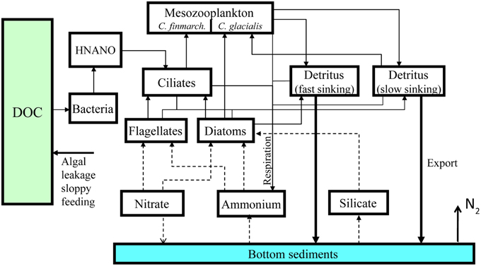
Figure 1. Ecosystem model structure. See text for details and explanations.

Model Set-up and Boundary Conditions

The model set-up encompassed the Nordic Seas, the central AO and the Eurasian shelf (Figure 2) and uses a horizontal grid point distance of 20 km. The model has 25 vertical levels. The levels which were modeled are the upper 10 m just below the sea surface, 10–15, 15–20, 20–25, 25–30, 30–35, 35–40, 40–50 m, then 50–75, 75–100, 100–150, 150–200, 200–250, 250–300, 300–400, 400–500, 500–700, 700–1000, 1000–1500, 1500–2000, 2000–2500, 2500–3000, 3000–3500, 3500–4000, and 3500–4500 m. Particular focus is provided to the region for which the SINMOD ecosystem model has been developed (and beyond), i.e., the western and eastern Fram Strait (FSW, FSE; where the main in- and outflow to and from the AO takes place), the southern and northern Barents Sea (BSS, BSN, permanently ice-free and seasonally ice-covered), the Laptev Sea Shelf Break (LSS, east-ward spreading of Atlantic water) and the North Pole (NoP, center point of AO) (see Figure 2).

FIGURE 2

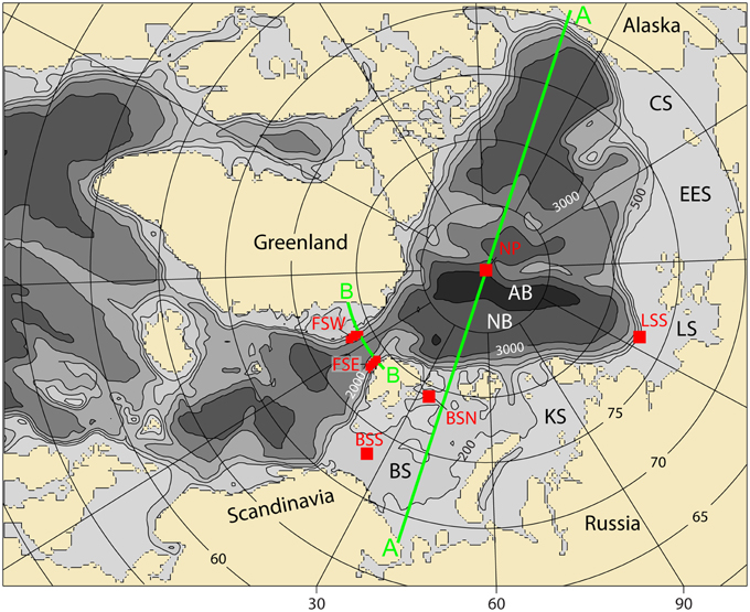
Figure 2. The model domain. BS, Barents Sea; SB, Spitsbergen; KS, Kara Sea; LS, Laptev Sea; ESS, East Siberian Sea; NB, Nansen Basin; and AB, Amundsen Basin. The transect line A (blue) indicates a cross Arctic Ocean transect. The transect line B (red) indicates a cross Fram Strait transect. The boxes indicate regions of 25 grid points that are investigated through a time series analysis: FSW, Fram Strait West; FSE, Fram Strait East; BSS, Barents Sea South; BSN, Barents Sea North; LSS, Laptev Sea Shelf Break; and NoP, North Pole.

A total of 8 tidal components were specifying and imposed (elevation and currents) at the open boundaries. Data were taken from TPXO 6.2 model of global ocean tides (http://www.coas.oregonstate.edu/research/po/research/tide/global.html).

Initial values of temperature and salinity are taken from World Ocean Circulation Experiment Global Data Resource Version 3.0 (http://www.nodc.noaa.gov). A comprehensive description of the WOCE data system can be found in Lindstrom (2001).

Fluxes through the open boundaries were kept constant during the simulation. A flux of 0.8 Sv enters the model domain through the Bering Strait (Woodgate et al., 2010). On the Atlantic side the average fluxes were taken from a large-scale (50 km resolution) model covering most of the North Atlantic. Part of the surface water heat advected into the Barents Sea, Svalbard. The model is also forced with freshwater fluxes (river discharges and diffuse run-off from land).

Freshwater run-off along the Norwegian coast and in the Barents Sea is based on data from a simulation with a hydrological model (see Dankers and Middelkoop, 2008 for more details). For Arctic Rivers, data are obtained from R-ArcticNet (Vörösmarty et al., 1996, 1998) available through http://www.r-arcticnet.sr.unh.edu/v4.0/index.html.

Two scenarios have been run: one presenting the present and past climate (1979–2010) and one the future IPCC Spres 2 scenario (A1B) from 2001 to 2099. The ERA INTERIM reanalysis (Dee et al., 2011; www.ecmwf.int) data (wind, sea level air pressure, air temperature, cloud cover, and humidity) has been used to force SINMOD in the first case. In the second case, the atmospheric forcing fields come from a regional model system run by the Max Planck Institute, REMO (Keup-Thiel et al., 2006). This model is configured to cover the model domain of SINMOD (Figure 2) and has a resolution of 0.22° and uses data from the MPI-ECHAM5 coupled climate model system.

SINMOD has open ocean boundaries to the Atlantic Ocean and the Bering Sea. The CARINA database (Tanhua et al., 2010) has been used to calculate the seasonal average of temperature (T), salinity (S), nitrate (NO₃), silicate (Si) (Bellerby et al., 2012). In order to depict the trends in nutrient concentrations at the boundaries we have used monthly mean values from Bergen Climate Model (BCM) using IPCC's A2 run for the climatic scenarios. Although these data are IPPC's A2 run, the development of atmospheric CO₂ concentration is quite similar to the A1B run (Nakićenović and Swart, 2000). Since these data had a significant offset compared with the CARINA data the BCM data has been corrected in the following way:

Using the CARINA data set the average values of T, S, NO₃, and Si for the 1990s around the model's open boundaries were calculated. The difference between these values and the BCM's A2 run was added to the BCM A2 boundary data for the Scenario runs. Since most of the CARINA data originates from the spring to summer season, the winter values were taken from the bottom of the winter mixed layer. The depth of the winter mixed layer in the North Atlantic was estimated based on Steinhoff et al. (2010). The CARINA data was also used for initial values of NO₃ and Si. The nutrient concentration (NO₃, Si) in the river run-off is taken from Dittmar and Kattner (2003) and Amon and Meon (2004).

Results

Before projecting the productivity of the AO into the future we need to examine if the SINMOD reflects the basic oceanography of today's AO. Thus, we start our attempt to characterize shortly the distribution and characteristics of various water masses in the AO of today through ERA INTERIM.

Simulated Monthly Means (T, S, and NO₃) Across the Arctic Ocean and the Fram Strait

Early spring and late summer data were selected for two cross sections. Section A starts in the Barents Sea (40°E) across the North Pole into the Beaufort Sea (140°W) and section B across the Fram Strait along at 79°N (Figure 2). Section A shows warm and saline water on the Barents Sea shelf having low stratification in winter, but strong stratification in late summer (Figure 3). A core of warm Atlantic water (AW) is locked to the shelf break north of Svalbard. This core is the east-bound, subducted AW, start of the boundary current that engirdles the entire AO. Along transect A two separated cores with AW are found across the AO, as indicated by elevated temperatures (Figures 3A,B). This is AW following the Gakkel and Lomonosov ridges toward Greenland. The boundary current on the Canadian side is clearly visible at depths of 300–800 m depth (Figures 3A,B). Toward the end of the summer, the temperature has increased to more than 6°C in the southern Barents Sea (Figure 3B). Strong stratification due to ice melt is encountered throughout the center of the AO (Figure 3D).

FIGURE 3

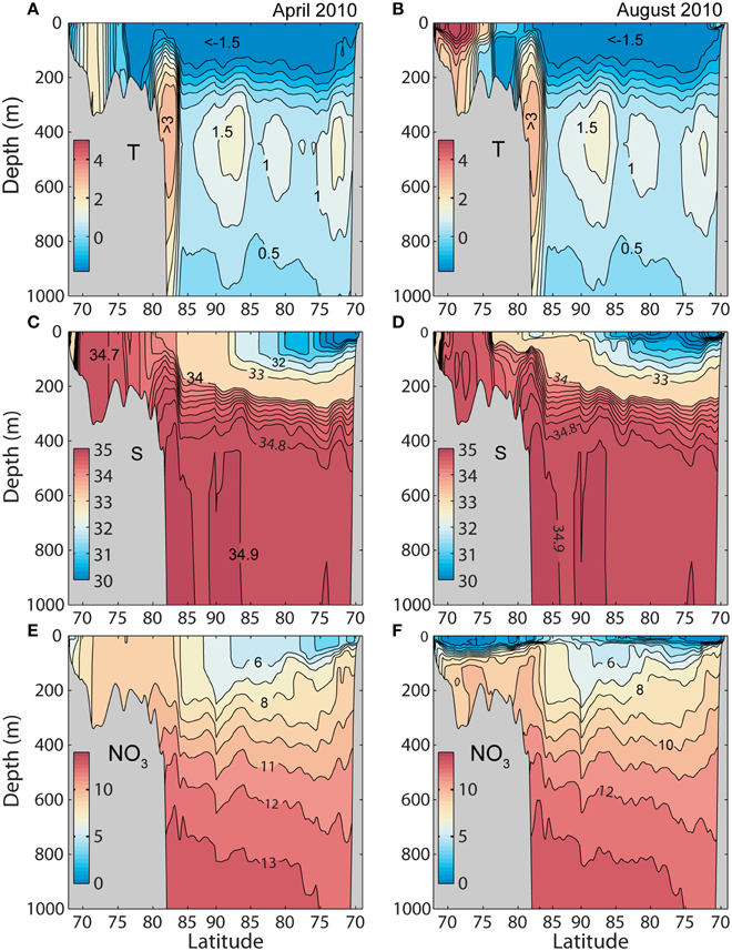
Figure 3. Simulated monthly mean temperature (°C), salinity (psu), and nitrate (mmol N m⁻³) along section A from the southern Barents Sea to the Beaufort Sea 2010 (see Figure 2), forced by ERA INTERIM (reanalyzed atmospheric fields). (A,C,E) April 13. (B,D,F) August 16.

The surface nitrate concentration is low in the AO and especially in the Beaufort Sea where it is low even in late winter (Figure 3E). In summer nitrate is removed from the near surface layer along the entire section, although some nitrate is still available between 85 and 90°N (40°E). Nitrate availability is relatively high on the Barents Sea side and depleted during the productive season, supporting a high new production.

Section B across the Fram Strait (along 79°N; Figure 2) shows typical AW in the eastern part of the section and low saline cold water originating from the Arctic in the western side, in particular on the Greenland shelf (Figure 4). Due to ice melt a shallow mixed layer is created in the western part of the section whereas surface heating seems to be the dominant factor for creating stability in the eastern, Atlantic part of the section. The winter concentration of nitrate is low in Artic water whereas the West Spitsbergen Current (eastern side) has concentrations typical for AW. During the summer the surface water is stripped for nitrate over the entire Fram Strait.

FIGURE 4

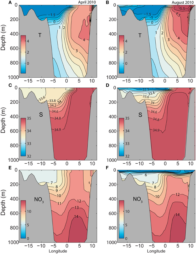
Figure 4. Simulated monthly mean temperature (°C), salinity (psu), and nitrate (mmol N m⁻³) along section B (79°N) across the Fram Strait 2010 (see Figure 2), forced by ERA INTERIM (reanalyzed atmospheric fields). (A,C,E) April 13. (B,D,F) August 16.

The described SINMOD results on basic distribution of water masses, water mass characteristics and currents of the entire AO (Figures 3, 4) are as reflected and interpreted by direct measurements (e.g., Schauer et al., 2008; Carmack et al., 2010; Carmack and McLaughlin, 2011; Mauritzen et al., 2011; Beszczynska-Möller et al., 2012; Woodgate et al., 2012; Smedsrud et al., 2013). This legitimates to investigate the future primary and secondary production.

A Comparison between ERA Interim and the A1B Scenario

In order to compare productivity derived from the hindcast (ERA INTERIM) with the forecast forcing (A1B) it is necessary to compare the two forcings for the same time interval (2001–2010). If there is reasonably coherence between the climate of the recent past then we may proceed with A1B forcing into the future. The A1B scenario is based on a “free running” downscaled version of the MPI Global atmospheric model. The ERA INTERIM (EI) is adjusted to the actual weather through data assimilation. The A1B data set covers a time period from 2001 to 2099 which make it possible to compare the average performance of the A1B forcing with the ERA INTERIM forcing.

Generally, as compared to the A1B-forced production, the ERA INTERIM-forced production is slightly lower in the Barents Sea and Arctic basins, but higher on the Arctic shelves (Table 1). The annual variability (expressed as STD) is higher in the ERA INTERIM-forced simulation run. In the Barents Sea the ERA INTERIM-forced annual average of GPP is 97 g C m⁻² (STD 7.6). The A1B forced annual GPP production is 104 g C m⁻² that is within the range of STD. In the Arctic basins the annual ERA INTERIM-forced GPP production is 17.3 g C m⁻² (STD 3.4), while the A1B-forced GPP production comprises 20.2 g C m⁻². On the Arctic shelves, which are dominated by the Siberian, shelf, the A1B run provided lower GPP (28.6 g C m⁻²) as compared to the ERA INTERIM run (32 g C m⁻²). Despite these differences the annual production rates of both forcings are similar and of same order.

TABLE 1

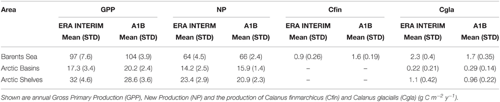
Table 1. Comparison between of simulated mean rates for the 2001–2010 period for ERA INTERIM and A1B for different regions of the AO [mean and standard deviation (STD)].

Simulated Monthly Means (T, S, and NO₃) Across the Arctic Ocean and the Fram Strait: Projections for Middle and End of the Century

Also in the future water masses on the southern Barents Sea shelf (between 70 and 74°N) will stay well mixed in late winter (April), while the temperature increases above 4.5°C in the 2050 and above 6.0°C in the 2099 (compare Figure 3A and Figures 5A,B). Salinity is above 34.8. In the northern Barents Sea (between 75 and 80°N) the April temperatures range between 0 and 1°C around 2050 and above 2.5°C in 2099. Also here the water column stays well mixed. At the shelf break a core of AW (T = 5.5°C and S = 35) is flowing eastward. In the present climate this warm core is isolated from the surface by a low salinity surface layer (Figures 3A, 5A,B). Already in 2050 the low saline surface water has disappeared and the AW is found from 500 m to the surface. The Atlantic layer in the AO is projected about 2°C warmer than today (Figure 3A) toward the end of this century.

FIGURE 5

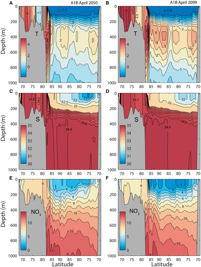
Figure 5. Simulated monthly mean temperature (°C), salinity (psu), and nitrate (mmol N m⁻³) for April along section A from the southern Barents Sea to the Beaufort Sea (see Figure 2). Forced by a A1B scenario. (A,C,E) April 13 in 2050. (B,D,F) August 16 in 2099.

Surface nitrate is slightly lower in the Barents Sea in 2050 and 2099 compared to today (Figures 3E, 5E,F), but the most pronounced difference is found in the AO. Today's low nitrate concentrations in the Beaufort Sea is encountered across the entire AO. Toward the end of the century, surface winter values of nitrate about 2 mmol N m⁻³ are found in the AO basins.

The model produces a structure of the West Spitsbergen Current (Figure 6) that is similar to the situation of today (Figure 4). The main difference is that the core temperature of the AW increases by about 3°C. The increased temperature of the Atlantic inflow is more pronounced toward the end of the century. SINMOD projects extremely low surface nitrate concentrations in the Arctic water (ArW) leaving the AO on and along the Greenland shelf in spring, about 3 mmol N m⁻³ around 2050 and 2 mmol N m⁻³ at the end of the century, respectively (Figures 6E,F). The surface water of the West Spitsbergen Current also contains less nitrate in the future, 1–2 mmol N m⁻³ less than compared to today (Figure 4E).

FIGURE 6

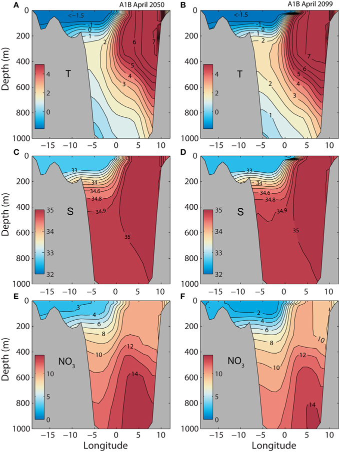
Figure 6. Simulated monthly mean temperature (°C), salinity (psu), and nitrate (mmol N m⁻³) for April along section across the Fram Strait (see Figure 2). Forced by a A1B scenario. (A,C,E) April 13 in 2050. (B,D,F) August 16 in 2099.

Time Variation of Ice and Productivity at Selected Arctic Ocean Regions

Before dealing with the productivity of the entire AO it is useful to address the variability of important processes at six selected sites that are inside or adjacent to the European Arctic Corridor (reaching from the Fram Straight to Severnaja Zemlja, east of the Kara Sea, Figure 2). To this end we characterize time series changes in ice cover (in spring and annually) and primary and secondary production (Figure 7). Each time series shows average values from an area of 10⁴ km². Two regions are in the Fram Strait (FSW, Fram Strait West; FSE, Fram Strait East). Two are in the Barents Sea (BSS, Barents Sea South; BSN, Barents Sea North). The two remaining regions are situated in the Laptev Sea (LSS, Laptev Sea Shelf Break) and at the North Pole (NoP, North Pole) (see Figure 7).

FIGURE 7

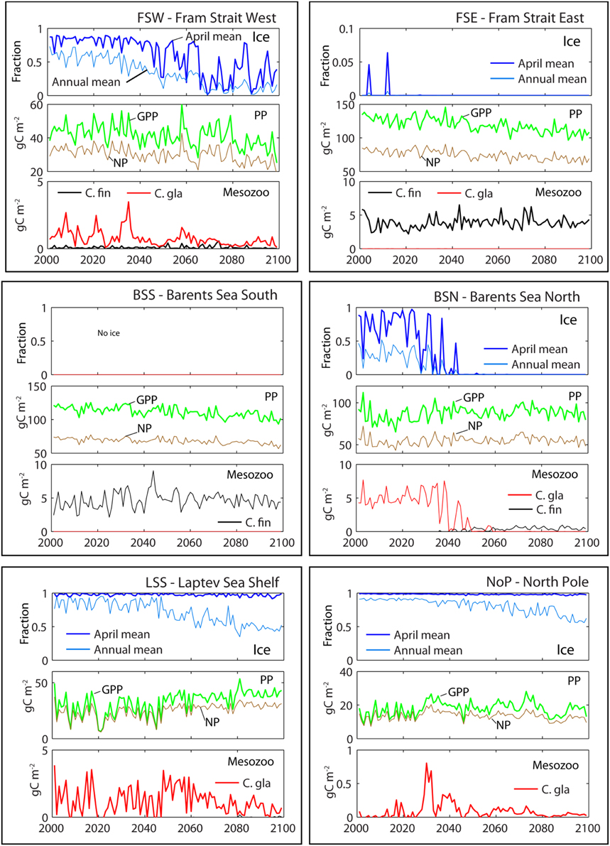
Figure 7. Time series variation at six stations in the Arctic Ocean. FSW, Fram Strait West; FSE, Fram Strait East; BSS, Barents Sea South; BSN, Barents Sea North; LSS, Laptev Sea Shelf Break; and NoP, North Pole (see Figure 2). Each of the six boxes shows the fraction of ice cover (above, 0–1), gross primary production (GPP, red) and new production (NP, blue) (middle; g C m⁻² y⁻¹) and the production of Calanus finmarchicus (C. fin., black) and Calanus glacialis (C. gla., red) (g C m⁻² y⁻¹). Forced by a A1B scenario.

Ice Cover

Both the annual mean and the April mean ice cover in the AO outflow region in the Western Fram Strait (FSW) is relatively stable to around 2040. After 2040 the April mean shows strong inter annual variability. The annual mean ice concentration decreases steadily with some interannual variability throughout the century (Figure 7, upper panels). The Eastern Fram Strait (FSE) and Southern Barents Sea (BSS) experience almost no ice. There is a large inter annual variability in the annual ice cover in the northern Barents Sea (BSN), which increases toward the 2040s. After 2045 the ice disappears completely from the BSN location. The April average ice concentration at the Laptev Sea Shelf break (LSS) shows no trends during the simulation period. However, the annual mean ice cover decreases from around 85% in 2040 to 50% in 2099. This reflects earlier break-up of winter ice and later refreezing during the autumn. At the North Pole (NoP) similar ice patterns are found. Annual mean ice cover will decrease from 95% in the 2040s to around 53% in 2099.

Gross Primary and New Production

GPP at FSW is characterized by great interannual variability (see Table 2 for average productions rates). There is a weak decrease in GPP toward the end of the century in spite of less ice cover (Figure 7, mid panels). The average NP is about 72% of GPP. GPP in the eastern part of the Fram Strait (FSE) is three times higher compared to the western part, but the NP is somewhat lower, 63% of GPP. The GPP in the southern Barents Sea (BSS) is similar to that of eastern Fram Strait (FSE). There is however a 14% decrease in production during this century.

TABLE 2

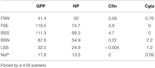
Table 2. Annual Gross Primary Production (GPP), New Production (NP) and the production of Calanus finmarchicus (Cfin) and Calanus glacialis (Cgla) (g C m⁻² y⁻¹) in the FSW, Fram Strait West; FSE, Fram Strait East; BSS, Barents Sea South; BSN, Barents Sea North; LSS, Laptev Sea Shelf Break; and NoP, North Pole, (2010; see Figure 2).

The mean annual GPP in the selected Northern Barents Sea station (BSN) is 87 g C m⁻² and surprisingly unaffected by ice conditions (Figure 7, mid panel). Even when the ice is completely absent the production does not increase. This is caused by southwards transport of ice-melt impacted surface water from the AO and lower winter concentration of NO₃. In the north-eastern Barents Sea the fresh water input is lesser and there we have a substantial increase in GPP (Figure 7). Average NP (63% of GPP) shows a minor negative trend with time. At the Laptev Sea shelf break (LSS) a significant increase in annual production from 25 to 40 g C m⁻² is projected around 2045. The ice cover decreases from 0.83 to 0.74 during the simulation period. The annual mean production at the North Pole (NoP) is 18 g C m⁻². There are relatively large inter annual fluctuations. The f ratio (NP/GPP) in the AO will decrease from 0.85 to 0.69 during this period. Most likely NP will decrease (nutrient limitation) while GPP increases (more PAR).

There is a strong decrease in GPP and NP along Section A (Table 3). In today's climate GPP ranges around 120 g C in the Barents Sea, 12 g C at the North Pole and 25 g C close to the Beaufort Sea shelf (m⁻² y⁻¹). The NP ranges from 78 and 11 to 21 m⁻² y⁻¹ at the respective stations. Across the Fram Strait there are also strong differences in GPP, with 120 g C on the Svalbard shelf and about 45 g C closer to Greenland (m⁻² y⁻¹, Table 4). Equivalent rates for NP is 79 and about 35 g C m⁻² y⁻¹, respectively. With an average f ratio of 0.76 it is obvious that NP in the AO represents a far higher proportion of primary production compared to boreal waters.

TABLE 3

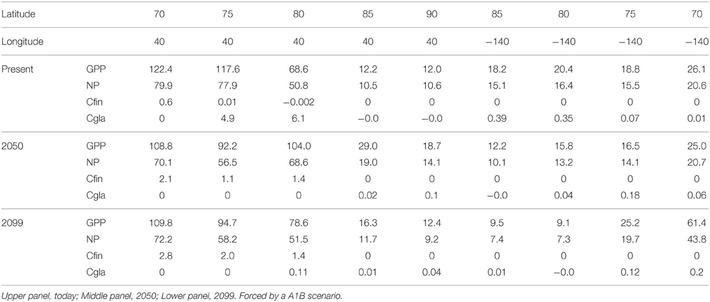
Table 3. Annual Gross Primary Production (GPP), New Production (NP) and the production of Calanus finmarchicus (Cfin) and Calanus glacialis (Cgla) (g C m⁻² y⁻¹) at the various latitudes along transect A from the southern Barents Sea to the Beaufort Sea (see Figure 2).

TABLE 4

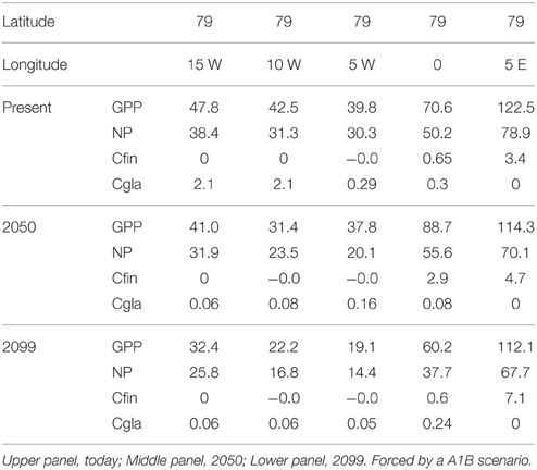
Table 4. Annual Gross Primary Production (GPP), New Production (NP) and the production of Calanus finmarchicus (Cfin) and Calanus glacialis (Cgla) (g C m⁻² y⁻¹) at the various latitudes along transect B across the Fram Strait (see Figure 2).

Production of Key Zooplankton Species

The mesozooplankton production is dominated by Calanus finmarchicus in the AW and C. glacialis in the ArW masses. In the Western Fram Strait (FSW) C. glacialis dominates, but shows large interannual variability (Figure 7, lower panels). There is a strong negative trend in production with time. In the eastern Fram Strait (FSE) production of C. finmarchicus is remarkably stable and very similar to the production pattern in the Atlantic dominated southern Barents Sea (BSS). In the northern Barents Sea (BSN) the mesozooplankton is dominated by C. glacialis. Around 2035 large oscillations in the production are seen for a period of 10–15 years. Note that the oscillations act in concert with the annual variation in ice cover. After this transition C. glacialis disappears totally from this location. C. finmarchicus is not able to replace C. glacialis since the temperatures here are not high enough for effective reproduction. The Laptev Sea shelf edge (LSS) has a significant production of C. glacialis, but the variability in production is extreme, from almost zero to 4 g C m⁻² y⁻¹ between consecutive years. Toward the end of the century there is a decrease in production even though annual mean ice concentration is decreasing. At the North Pole (NoP) we find a very low zooplankton production, caused primarily by low GPP. During the transition from permanent ice cover to periods with some open water around 2030 there is a short period with higher annual production (0.5–0.8 g C m⁻² y⁻¹).

The production of C. finmarchicus is connected to the warmer AW and thus only prominent in the Barents Sea station of Sector A (Table 3) and Svalbard, Sector B (Table 4). C. glacialis plays a more pronounced role along both transects, except at the stations dominated by AW. Dependent on both primary production and lower temperatures C. glacialis production is highest close to the northern Barents Sea and eastern Greenland shelf edge (Tables 1, 2).

Present and Future Annual Primary and Key Zooplankton Production in the Entire AO

No place is the GPP of the AO higher than across the western and central European Arctic Corridor, which is a continuum of highly productive regions along the Norwegian coast and the Norwegian Sea. Also in the advective regions of the Chukchi Sea and adjacent Bering Strait GPP is high (Figure 8, upper panel). In contrast, much lower GPP is found in the Arctic basins (10–20 g C m⁻² y⁻¹). Present GPP in the eastern Fram Strait, the southern Barents Sea and the Chukchi Sea are in order 120–150 g C m⁻² y⁻¹ and about 60 g C m⁻² in the northern Barents and Chukchi Seas. NP estimates show a similar pattern as GPP, which comprises around 62% of GPP in AW of the European shelf (Figure 8, lower panel). This percentage increases northwards toward the central AO where PAR is increasingly the limiting factor for production today.

FIGURE 8

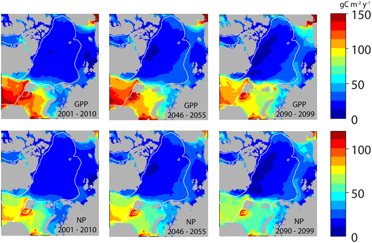
Figure 8. Simulated 10 year mean production gross primary production (GPP, upper panels) and new production (NP, lower panels) in the entire Arctic Ocean (A1B) at present (2001–2010), in 2046–2055 and 2090–2099 (g C m⁻² y⁻¹).

The intensification of GPP and NP in the AO basins during the course of this century is clearly illustrated in Figure 8. By 2050 GPP and NP have significantly increased north of Svalbard, the north-eastern Barents Sea, the Kara Sea Chukchi Sea and at the western end of the Siberian shelf. There is also an increase in the outer sections of the AO basins, but the basic pattern—low productivity in the center and highest production along the European Arctic Corridor region—prevails. Noteworthy is the decrease in GPP and NP in wide regions of the southern Barents Sea toward the end this century (Figure 8). North of Greenland and Canada GPP are low at present and it will decrease to about 10 g C m⁻² y⁻¹ toward the end of the century. Despite the general reduction in ice cover in the central AO the production is kept low due to limited supply of nutrients (see Figure 11).

At present high production of the Atlantic key mesozooplankton C. finmarchicus, closely connected to the warm AW masses, is found in the eastern Norwegian Sea and Fram Strait and southwestern Barents Sea (Figure 9, upper panel). The production here is in the range of 4–10 g C m⁻² y⁻¹. C. finmarchicus may also be found outside the AW, but the production is strongly reduced when summer temperatures stay below 4–5°C. Along and toward the Eurasian shelf break its production is negative (growth—respiration). Today's production of the Arctic species, C. glacialis, is high north of the Polar Front, in cold ArW and the northern Barents and Greenland Seas (Figure 9, lower panel). This species is also found along the Eurasian shelf, but in much smaller quantities. Production along the Siberian shelf break is negative.

FIGURE 9

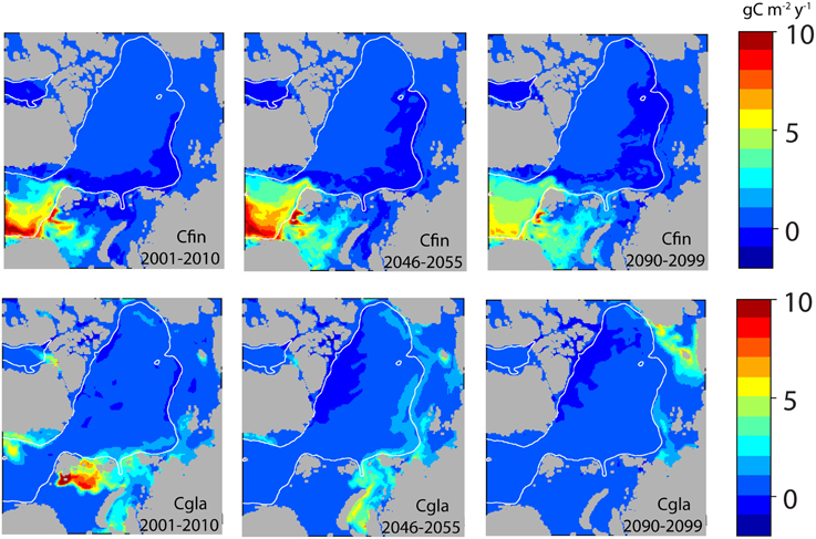
Figure 9. Simulated 10 year mean annual production of the zooplankton key species Calanus finmarchicus (Cfin, upper line) and Calanus glacialis (Cgla lower line) in the entire Arctic Ocean (A1B) at present (2001–2010), in 2046–2055 and 2090–2099 (g C m⁻² y⁻¹).

Toward the end of the century and along with warming (Figure 10) the production areas of C. finmarchicus will gradually expand into the Greenland Sea, northern Barents Sea and even the western Kara Sea (Figure 9, upper panel). The production in the southern Barents Sea and western Fram Strait suggests a negative trend. As AW spreads eastward north of Svalbard along the northern edge of the Barents and Kara Seas (Figure 10), negative production is turned into net growth. The area of negative growth is now found further east along the shelf break (Figure 9). There is a significant increase in the production of C. finmarchicus in the northern Barents Sea, but the temperature is too low for effective growth (Figure 10).

FIGURE 10

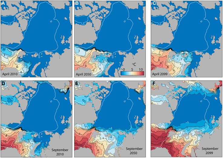
Figure 10. Monthly simulated mean surface water temperatures at the start of the productive period in April (upper panel) and at the end, September (lower panel) in the entire Arctic Ocean (A1B) at present (2010), in 2050 and 2099 (°C).

C. glacialis is sensitive to increased water temperature. Already in 2055 most of the Barents Sea population has disappeared (Figure 9). There is a transition to a gradually more eastern distribution. Around 2055 we find a substantial production of C. glacialis in the Kara Sea. Forty years later the production of C. glacialis has collapsed also there (Figure 9). The production in the Kara Sea region is stable to around 2050 when a steady decline start accompanied with larger inter annual oscillations until complete stop in production by 2080 (data not shown). The production areas of C. glacialis have by then moved along the Siberian Shelf and into East Siberian Sea, especially near the shelf break (Figure 9).

The productivity of C. finmarchicus and C. glacialis along Section A and B in 2050 and 2099 are in principle similar to those of today (Tables 2, 3), but show some clear deviations. C. finmarchicus expands from 70 to 80° latitude in 2050 and 2099 while C. glacialis disappears from these stations, but produces throughout the remaining section (Table 3). Along section B no principle changes are projected by 2099, but C. finmarchicus intensifies its production close to Svalbard while production of C. glacialis appears to cease throughout (Table 4).

Discussion

Since the beginning of the twenty-first century the Arctic became warmer and wetter, a self-reinforcing trend expected to continue because it is linked to sea-ice melt and more persistent open-water conditions (Boisvert and Stroeve, 2015). Recent awareness of rapid climate change in the AO, the most significant on the globe, is accompanied by the fact that the region has critical effects on the biophysical, political, and economic system of the Northern Hemisphere (such as increased winter storms, record snow falls). Extreme weather events in the midlatitudes are linked through the atmosphere with the effects of climate change in the Arctic, such as dwindling sea ice (Grambling, 2015). The continuous melt of sea ice, in particular the expected disappearance of summer ice, an extensive open water region, a “new ocean,” that due to massive ice-cover were not managed by the nations that engirdle and use the AO. As we already see human activities spread in to the up till now ice-covered regions (e.g., oil/gas exploitation, shipping, fisheries, tourism) the demand to obtain sufficient system-ecological knowledge is paramount. Humanity has to apply the limited knowledge regarding the AO (Wassmann et al., 2011) and tools in all possible manners of which physical-biologically coupled modeling is one. In order to guide future management, investigating the physical constrains and production over the entire AO is imperative.

Confines and Limitations

We have presented results from SINMOD using forcing from a single downscaled A1B scenario of the global climate model MPI-ECHAM5. It is well known that there are many uncertainties associated with these climate model scenarios and we will point to those of greatest relevance for the present study. We have chosen the A1B emission scenario as the CO₂ emission over the latest years follows this rather pessimistic projection. Only a single model simulation was run and this must be considered. Running an ensemble of simulations would enable us to provide more robust trends over time. This would be a very computational demanding task and as the purpose of the present analysis is to discuss the physical constrains of the future production and not to determine the general trends, a single simulation is adequate.

A well-known atmospheric feature in the AO is the Beaufort High located over the Beaufort Sea (Kwok, 2011; Wood et al., 2013). This weather system transports ice toward the Canadian Archipelago. Kwok (2011) compared results from CMIP3 model runs with observations and found that the mean high-pressure system was in most models displaced. The MPI-ECHAM5 has the high-pressure center displaced toward the central Arctic and this influences naturally SINMOD ice results both by direct wind driven forcing, but also because SINMOD ice distribution will resemble the ice cover of the forcing data due to thermodynamics. Another aspect is the rapid decrease in the observed ice cover that is not captured by most global models (e.g., Carstensen and Weydmann, 2012; Wadhams, 2012; Kwok et al., 2013), which is also the case for the SINMOD results presented here. Future projections of primary production are naturally sensitive to model presentation of ice and Vancoppenolle et al. (2013) characterized ice cover to be the largest source of uncertainty.

Consideration of computational time for a model run for 1970 to 2100 for the entire AO resulted in that only a horizontal resolution of 20 km was chosen. However, the internal Rossby radius in the AO is around 10 km and thus the applied resolution is too coarse to resolve eddies. Eddies are important for mixing and cross shelf transport. This probably has an effect on the present simulations. When the grid size of the original model was changed from 20 (e.g., Slagstad and Wassmann, 1997) to 4 km (e.g., Wassmann et al., 2006b) GPP increased on average with 14.5%, mainly due to eddy resolution. However, interannual variability was similar and on regional scales, the spatial distribution of GPP was the same. Higher productivities can be expected if the spatial resolution of the model increases, in particular on shelves, shelf seas and water columns that are weakly stratified.

SINMOD does not account for vertical mixing by internal waves and vertical transport by double diffusive convection. Including both processes into the vertical mixing scheme of the model is non-trivial, as discussed in Sundfjord et al. (2008). That SINMOD potentially underestimates mixing can be overrun by an “artificial” vertical mixing that occurs as a consequence of representing vertical motions in a z-level model. GPP results from SINMOD might thus be both over and underestimated due to this. Given that the model give a realistic water mass distribution implies that this error should not have a significant impact on spatial distribution of GPP.

The model results are sensitive to light attenuation in ice and ice-covered water and this creates challenges for modeling primary production (Babin et al., 2015). Besides shading by plankton and ice algae PAR underneath ice depends on ice thickness and snow on the ice surface. SINMOD gives an annual mean gross production rate of 16 g C m⁻² y⁻¹ in the Arctic basins. The production is relatively sensitive to the assumptions of chosen attenuation coefficient through ice (Pegau and Zaneveld, 2000). A doubling of the attenuation coefficients results in a production of 9.6 g C m⁻² y⁻¹ and reduction of 50% to a production of 26 g C m⁻² y⁻¹, which is similar to the A1B projection toward the end of the century. Whatever, the realism of the applied PAR model, GPP and NP will stay low as long as ice-cover prevails.

Another source of uncertainty is related to that the SINMOD was used for the entire AO using the same ecosystem structure and parameter settings. The further we move from the European Arctic Corridor into the AO the more questions may be raised about the adequacy of the applied biological model. However, SINMOD does not differ significantly in structure compared to other models used for pan Arctic studies and produce generally similar distribution of GPP (Babin et al., 2015). The greatest weakness that is important to keep in mind is that the model underestimates production in the Chukchi and the Beaufort Sea. There are several potential reasons for this. One is that the open boundary of the model domain is too close to the Bering Strait. In the shallow Chukchi Sea there is also a close pelagic-benthic coupling not properly represented in SINMOD.

In this model primary production does not distinguish ice algae from plankton algae as only phytoplankton is considered. Primary production in the AO can comprise significant fractions that derive from ice algae (e.g., Tedesco et al., 2010, 2012; Leu et al., 2015). During the Arctic melt season, floating ice algae aggregates likely play an important ecological role in an otherwise impoverished near-surface sea ice environment (Boetius et al., 2013; Assmy et al., 2014). The timing of phytoplankton and ice algae blooms as well as the biochemical composition is different. As we cannot distinguish between these two algae forms only annual primary production estimates are presented, which do not depend on such a differentiation.

The robustness of SINMOD of answering how much annual productivity will change in a future AO. Where the changes may be observed is not fundamentally different from other projections (i.e., Vancoppenolle et al., 2013). Our simulations seem thus adequate to approximate possible scenarios of productivity in the future AO. Our main goal is to point out the all-over trends and spatial patterns in productivity around the high-productive perimeter of the AO basins and a discussion on the changes in forcing that result in the expected patterns.

Physical and Chemical Changes in the Future Arctic Ocean

Strong stratification preventing mixing between surface Polar Water and the nutrient-rich halocline water below are one of the main characteristics of the AO, except for sections of the inflow shelves (Carmack and McLaughlin, 2011).

There are several factors that impact freshwater content in the AO and thus the surface salinity and stratification (e.g., Carmack et al., accepted). Freshwater run-off from land is locally important, but most of the AO freshwater ultimately derives from the Pacific Water inflow. Freshwater in sea ice is a minor fraction (Figure 11B). Stratification in the upper 100 m is thus only partly influenced by Pacific Water and ice melt, the latter in the uppermost meters. Ice dynamics, strongly impacted by wind, are an important forcing factor for the surface freshwater distribution. It results in freshwater and ice accumulation close to northern Canada and Greenland, causing both considerable light and nutrient limitation. Sea ice cover can thus be primarily wind or thermally driven, or both (Frey et al., 2015).

FIGURE 11

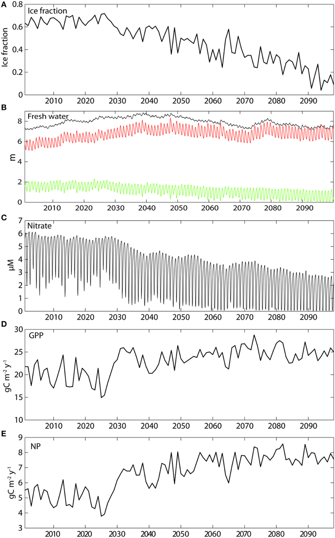
Figure 11. Mean annual simulated ice concentration for April (%, A), the total (black), liquid (red), and ice (green) bound freshwater heights in the upper 100 m of the water column using a reference value of salinity of 35 (B), the nitrate surface concentrations (C), and the annual gross primary (D) and new primary (E) productions (g C m⁻² y⁻¹) in the Arctic Ocean basins throughout this century (A1B).

Increased stratification results in decreasing simulated nutrient concentrations in the upper water masses, particularly in the basins of the AO. A steady decrease during this century is projected (Figure 11C). As summer ice gets thinner and eventually disappears (Figure 11B), primary production will increase because of increased PAR, but become increasingly nutrient limited. In today's climate surface nitrate concentrations decrease during the growth season to about 2 mmol m⁻³. By about 2050 nitrate concentrations may become undetectable at the end of the growth season while the maximum concentration will drop from 6 to 4 mmol m⁻³ (Figure 11C). This estimate is supported by Vancoppenolle et al. (2013) who suggests that the AO surface NO₃ concentrations decrease over the twenty-first century by 2.31 mmol m⁻³, associated with shoaling mixed layer and with decreasing NO₃ in the nearby North Atlantic and Pacific waters. The estimate is almost identical with results from SINMOD (Figure 11C). In the AO basins increased stratification and significant nutrient limitation will characterize an AO free of summer ice, a likely scenario within the next decades. This impoverishment of nutrients impacts NP. So even though increased wind driven mixing is expected as the summer ice-free area in the AO expands and in the AO basins internal motions may contribute to mixing, (e.g., Rainville et al., 2011), it is not necessarily enough to support large increase in GPP. Even though there are errors in the atmospheric forcing fields as discussed in 4.1, these same results were achieved with a model experiment using ERA-INTERIM forcing where air temperature artificially was increased to obtain ice free summers (Slagstad et al., 2011).

What impact the increase in PAR and UVB will have on phytoplankton growth and diversity remains a matter of discussion. Whereas Arctic warming is expected to lead to lower net community production (Vaquer-Sunyer et al., 2010, 2013), recent experimental results suggest that increased UVB radiation may partially stimulate primary production in surface waters (Garcia-Corral et al., 2014). In the central AO SINMOD projects only a slight increase in GPP and NP of 20–25 and 5–8 g C m⁻² y⁻¹ during the course of this century, respectively.

Primary Production of the Future Arctic Ocean Basins

The development of ice cover, primary and secondary production in the course of this century demonstrates clearly that the AO is highly dynamic spatially variable and affected by ice cover (Figure 7). Throughout this century GPP and NP range widely between a few to 150 and 100 g C m⁻² y⁻¹, respectively, with the highest rates on the shelves and seas of the European sector to the Arctic Ocean and the Chukchi Sea (Figure 8). In essence, SINMOD suggests that primary production increases in most regions (in particular along the northernmost shelves and shelf breaks), that it declines in the southernmost regions in the European sector and north of Greenland and Canada, but that the basic production patterns in the basins will only change slightly (Figures 8, 13A).

In the present climatic regime the simulated GPP and NP for the entire Arctic basins are for the most limited by PAR, but later nutrient depletion plays a role (Figures 11A,C). Along with the declining ice cover in the AO basins (from 0.6 to 0.1 ice fraction) also the winter concentrations of nitrate decline (from 6 to 2.5 mmol m⁻³; Figure 11C). Widespread nitrogen deficiency in surface waters fosters the occurrence and seasonal persistence of subsurface layers of maximum chlorophyll a and phytoplankton carbon biomass (Tremblay et al., 2015). From about 2050 and onwards surface water nitrate gets depleted after the spring bloom, clearly indicating an increasing nutrient depletion in the AO basins throughout this century. The decrease coincides with the decline in ice cover around 2025. The reason of increasing nutrient depletion while radiation and GPP increases (Figure 11D) is found in the highly stratified nature of the AO basins (Figures 3, 5). Large amounts of freshwater (7–8 m) characterize the upper 100 m of the AO basins from which the ice fraction only comprises 0–2 m (Figure 11B). As a result of increasing light availability and stratification surface waters get stripped for increasing amounts of nitrate through modest, but inevitable sedimentation. Which has implications for regenerated production and the potential NP the following year. As a consequence, the new (or harvestable) production increases only by about 2 g C m⁻² y⁻¹ in the AO basins over the course of this century (Figure 11E). This is reflected in the negligible to small difference of GPP and NP in the central AO basins between 2001–2010 and 2091–2099 (Figures 12A,B). The entire basin area does not enjoy major increases of primary production and toward northern Greenland and Canada even decreases are projected. These results, all connected to the on-going and future freshening of the AO are much in line with suggestions by Coupel et al. (2015) for the Pacific AO.

FIGURE 12

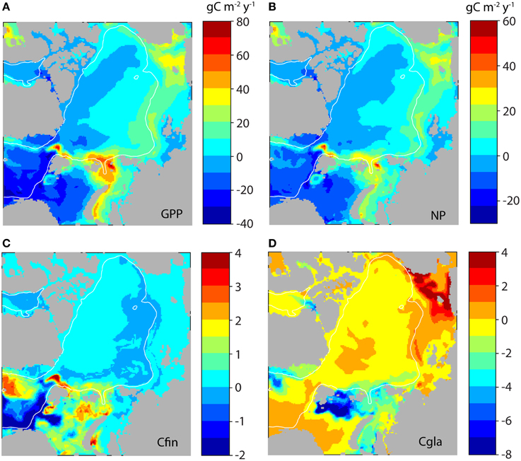
Figure 12. Difference between the simulated gross primary production (GPP, A) and new production (NP, B) between 2099 and 2010 (as based upon Figure 8; g C m⁻² y⁻¹). Also shown is the difference between simulated production of Calanus finmarchicus (Cfin, C) and C. glacialis (Cgla, D).

The average GPP in the Arctic basins increases slightly from 19.5 to 23 g C m⁻² y⁻¹ around 2030 (Figure 11D) that is also reflected by the North Pole station (Figure 7, station NoP). This is mainly caused by a small drop in ice summer concentration that allows more PAR to penetrate into the water column. After 2030 the model suggests summer ice concentration in the Arctic basins to decline continuously and, switching from light to a nutrient limitation, the average GPP remains close to 23 g C m⁻² y⁻¹.

The change from light to nutrient limitation is reflected by the f ratio. The f ratio is far higher in the AO as compared to boreal sea regions. This difference is due to the short growth season in which spring production (high f ratio) constitutes a substantial proportion of GPP at higher latitudes. Regenerated production during a short summer–fall period is correspondingly less important. As a consequence the f ratio in today's AO basins is comparatively high. More light availability and nutrient depletion the f ratio drops significantly during this century. With a harvestable production over the entire AO basins in the range of 4–8 g C m⁻² y⁻¹ (Figure 9) and neutral or slightly increasing trends in the projections for this century (Figure 11D) the potential for a sustainable pelagic fishery in the AO basins is small. By large the SINMOD results support the conclusion of Coupel et al. (2015) that predicted an increase in freshening in future years will likely cause the Arctic deep basins to become more oligotrophic, caused by weaker surface nutrient renewal, despite higher light penetration.

The Hot Perimeter of the Future Arctic Ocean Basins: Primary Production along the Eurasian Shelf Break and Adjacent Shelf Seas

While there is general agreement that primary production will stay low in the central AO basins, even when summer ice retreats for good in forthcoming decades, the question can be raised where the differences between today's and future climate may be strongest? The major increases in GPP and NP will take place at the Eurasian perimeter of the AO, in particular along the shelf break and adjacent shelf stretching from the Beaufort to Svalbard, including the southern Kara Sea (Figures 12A,B, transect A in Figures 13A,C). These are not only the regions where ice loss and PAR gain will be greatest. Shelf seas and particularly along shelf breaks are also regions where advection of AW and PW is most significant and where vertical density gradients are less pronounced, leading to vertical mixing and upwelling. This is illustrated by increasing GPP and NP between 80 and 95°N along transect A (Figures 13C,D). The difference in productivity between the Eurasian and American-Greenlandic perimeter across the Fram Strait is strong and this pattern will continue (Figures 13B,D). However, increasing stratification over the course of this century (e.g., thermal generated on the Svalbard and due to ice-melt in the Greenland side) suggests a generic, Fram Strait wide decrease in primary production (Figures 13B,D). The perimeter of the AO has a hot (Svalbard to Beaufort Sea) and a cool side (northern Greenland and north eastern Canada). Of particular interest is the increase in productivity along the Siberian shelf break (around 80°N) in the latter part of this century (Figure 8).

FIGURE 13

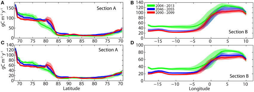
Figure 13. Annual simulated gross primary production (GPP, upper panel), new production (NP, lower panel) along transect A (A,C) and transect B (B,D) (Figure 2) for the period 2001–2010 (green), the period 2046–2055 (blue) and the period 2090–2099 (red). The shaded areas correspond to the period mean values are ± one standard deviation.

The increases in productivity may support increased harvestable production for some Arctic countries such as Norway, but in particular north-western Russia, including the Kara Sea, will experience a pronounced increase of harvestable production caused by climate warming (Figures 12A,B, 13). These regions will be characterized by a harvestable production range of 80–100 g C m⁻² y⁻¹ (Figure 8B), comparable to today's regions with significant fisheries (such as the Barents Sea and eastern Fram Strait). The production in the Chukchi Sea is high today and will increase in the future, but that does likely not result increased fisheries as a cold pool in the Bering Strait prevents the spread of commercial fisheries into the AO (Hunt et al., 2013). Over the next 30–50 years Skaret et al. (2014) predicted an all-over increase of GPP in a major fraction of the Barents Sea of about 36% (in some regions from 100 g C m⁻² y⁻¹ to around 200 g C m⁻² y⁻¹). The majority of this production will take place in the ice-free region in the south. In contradiction, toward the end of the century SINMOD predicts a decline for the entire Barents Sea of 9% and for the hitherto ice-covered north-western Barents Sea an increase of 8% (results not shown). Differences in physical forcing is part of the reason why two models using the same IPPC scenario provide contradicting results, but the mechanism for how additional nitrate can be added to the upper layers of the ice-free Barents Sea in times of warming (advection of AW and increased heat flux from the atmosphere) is not provided (Sandø et al., 2014; Skaret et al., 2014). On the contrary, winter nutrients in the Atlantic waters of the Barents Sea have declined from 1990 to 2010, silicate about 20% and nitrate by about 7% (Rey, 2012). This is caused by changes in the Atlantic inflow waters, which originate much further south in an North Atlantic subjected atmospheric changes. Also cloud cover and PAR must not be forgotten. Increasing cloudiness in the Arctic dampens the potential increase in phytoplankton primary production caused by receding sea-ice (Bélanger et al., 2013). Consistent with these declines SINMOD predicts a decrease of GPP and NP over the next 100 years in the southern Barents Sea and adjacent regions. As ice disappears and the Polar Front moves northwards (Wassmann et al., 2015), primary production in the north increases, as predicted by Skaret et al. (2014). Primary production estimates are sensitive to how well the model performs with regard to physical environment (Popova et al., 2012, 2013), in particular vertical mixing (see Physical and Chemical Changes in the Future Arctic Ocean). Therefore, in the future more care has to be taken to ensure that the physics of models are as correct as possible.

In the AW that dominates the south-western Barents Sea GPP is nutrient limited after the spring bloom. Nutrient availability is determined by (i) winter concentration of nutrients of AW, (ii) the strength and onset of thermal stability during early summer and (iii) the nutrient concentration of the inflowing water (e.g., Rey, 2012). In AW dominated parts of the Barents Sea and eastern Fram Strait vertical mixing in the weakly stratified water column reaches down to 200 m and more (Figure 14). Any change of AW warming (surface) will increase thermal stratification. As a consequence of warming, SINMOD simulates a decrease in GPP during this century partly due to decreased winter nutrient concentration of AW (Figure 8). Already at ocean weather ship Mike (66°N, 2°E) in the inflow region of AW of the Norwegian Sea the effects of increasing thermal stratification can be shown by SINMOD, with a reduction of the maximum nitrate concentrations of 1 mmol m⁻³ during this century (results not shown). This effect, already observed (Rey, 2012), becomes more pronounced in the southern Barents Sea (Figure 14). SINMOD suggests that the maximum nitrate concentrations decrease in the bottom and surface waters with about 1 mmol m⁻³ during the century, and the main reason for this may be increased thermal stratification projected by SINMOD. A future increase of primary production in AW would require increased frequency of intense wind events during to break down thermal stability. Previous simulations (Wassmann et al., 2006b) have shown that the thermocline during summer is quite persistent and an effect of wind-induced mixing is greatest during early spring and summer (Sakshaug et al., 2000).

FIGURE 14

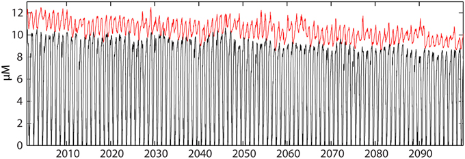
Figure 14. Variation of simulated nitrate concentrations (μM) near the bottom between 300 and 370 m (red) and at the surface (black) in the southern Barents Sea during this century (A1B).

The increase in GPP along the European and Siberian perimeter is predicted to range between 20 and 80 g C m⁻² y⁻¹ and decrease by up to 30 g C m⁻² y⁻¹ in the regions dominated by AW inflow or ArW export. Where these changes can be observed is highly variable and depends upon the selection of stations for time series studies (Figures 2, 14, Table 2). There is also significant interannual variability reflecting the dynamic nature of climate–enforced primary production.

The basic feature of future changes in GPP and NP are thus a decline in the southern AW (caused by thermal stratification) and north of Greenland and Canada (accumulation of ice), and a crescent shaped increase region along the Eurasian and American continental shelf (caused by reduction in sea ice, increased vertical mixing, and upwelling along shelf break).

Secondary Production of the Future Arctic Ocean

The secondary production estimates of SINMOD have to be interpreted with great caution. Regarding physical forcing and primary production the knowledge from the Barents Sea and adjacent regions can be more straightforwardly applied over large arctic region. However, this is more complicated for various species of copepods. While the Calanus finmarchicus model is adequate for the regions dominated by AW (comprising a large share of the secondary production in the AO), the case of Calanus glacialis is more complicated. C. glacialis is assumed to be a shelf species, but in the model it represents Arctic copepods per se, despite of being only one of several Arctic species. For example, the important, long-lived C. hyperboreus that inhabits the deeper waters of the AO, the Fram Strait and adjacent Greenland Sea is not part of the model. The results of SINMOD can thus predict with some certainty the future development of C. finmarchicus and C. glacialis along the European Arctic Corridor (where most of the AO secondary production takes place), but the predictions for C. glacialis beyond this region have to be interpreted as an indication for the potential secondary production of unspecified Arctic copepods.

Toward the end of this century the production of C. finmarchicus is predicted to increase substantially in the Greenland Sea, north and south of Svalbard and the eastern Barents Sea, which finds support by Skaret et al. (2014). The eastern extent of C. finmarchicus production is found in the St. Anna Trough and has to be seen as a result of warming (Figure 10). There is an obvious decrease in C. finmarchicus production in regions that in today's climate play an important role for fish food and fisheries (e.g., Figures 8A,B). This points at that we may expect a decrease in C. finmarchicus as fish food in these regions (Figure 12C), which is in contrast to Skaret et al. (2014). As mentioned above the reason for the decline in NP and secondary production is caused by the increased thermal stratification and the 15–20% decline in nitrate of the AW that is advected into the Barents Sea (Figure 14). Biomass of C. finmarchicus is advected further east along the shelf break, but the temperature in this area is not sufficient for build-up of new biomass: respiration losses exceed production. This is seen as tongue of negative production rate along the shelf break (Figure 12C). Today's significant production of C. glacialis (Figure 12D) is strongly reduced in the northern Barents Sea (i.e., C. glacialis disappears completely from these regions). Increase in production is found along the Laptev-East Siberian shelf break (e.g., Kosobokova et al., 2011). Being part of the hot AO perimeter, it will here create a new food source for pelagic organisms, while production is low and negligible along the American-Greenlandic perimeter. Should these predictions become a reality or unless other zooplankton species of comparative nutritional significance substitute future fishery management in the AO will have to be re-evaluated.

Projections of Arctic Ocean Productivity toward the End of the Century

Despite the limitations and shortcomings that are connected to any model that attempts to project the future our SINMOD projections for C flux and productivity in the future AO are useful to address the main goal. This is to point out the all-over time trends, the approximate order of changes and future spatial patterns in C flux and productivity along the high-productive perimeter of the AO basins.

Local changes in light availability resulting from reduced sea-ice are only one factor in the intricate web of local and remote drivers of GPP and NP in the Arctic Ocean. GPP and NP increase along the Eurasian perimeter of the AO basins and adjacent shelf seas, in particular in the northern Barents Sea and entire Kara Sea and the projected increases are in the range of 10–80 g C m⁻² y⁻¹ and 10–50 g C m⁻² y⁻¹ of GPP and NP, respectively (Figure 12). The central regions of the AO, subjected to increasing freshening, show a slight increase in GPP while NP does hardly change. On the American-Greenlandic perimeter of the AO GPP and NP are projected to decrease to even lower rates, mainly due to continued ice-cover and freshening. In the southern regions of the continuous domains of AW advection, in the outflow regions east of Greenland and compared to today's productivity GPP and NP will generally decline, caused by increased thermal stratification and declines in the advected nutrient concentrations.

The increase in GPP and NP along the shelf break and adjacent continental shelves of Eurasia is accompanied by increased productivity of zooplankton in the range of 1–4 g C m⁻² y⁻¹ (Figure 12). The hot perimeter of the AO may thus support increased growth of pelagic species that are of commercial interest, such as cod and capelin, but ultimately also shrimps, snow crab, and scallops (see also Renaud et al., 2015). Among the Arctic coastal nations Russia may benefit the most from the increases in harvestable production in the future AO. A sustainable pelagic fishery in the central AO basins appears unlikely, as harvestable production at best will stay low and may even decline.

The Atlantic copepod species Calanus finmarchicus will expands its dominance in the Barents Sea, the Greenland Sea and adjacent regions, but will not penetrate into the central AO and only by advection along the Siberian shelf. Arctic zooplankton, here exemplified by Calanus glacialis, will increase its abundance over much of the AO, in particular the Eurasian shelf and shelf edge. In the most productive fishing regions of the Arctic and Sub-Arctic these two species play a pivotal role today, but this may change in decades to come, resulting so far unidentified consequences for zooplankton consumers such as capelin, juvenile fish and marine birds.

Conflict of Interest Statement

The authors declare that the research was conducted in the absence of any commercial or financial relationships that could be construed as a potential conflict of interest.

Acknowledgments

This work was funded by the European Union through the project Arctic Tipping Points (ATP, contract # 226248; www.eu-atp.org) in the framework FP7, the projects CarbonBridge and ARCEx—The Research Center for ARCtic Petroleum Exploration funded by the Research Council of Norway (contracts # 226415/E10 and #228107, respectively), and Arctic Climate Change, Economy and Society (ACCESS, contract # 265863). It is also a contribution of the ARCTic marine ecOSystem research network, ARCTOS (www.arctosresearch.net), a northern-Norwegian network that emphasizes interdisciplinary approaches to addressing large-scale and pan-Arctic questions in marine arctic oceanography. We acknowledge the contribution of R. Bellerby and A. Silyakova inside the frame of the Research Council of Norway funded project Marine Ecosystem Response to a Changing Climate (MERCLIM, contract # 184860), resulting in a better-constrained SINMOD model. Three anonymous referees contributed significantly to the improvement of the manuscript.

Footnotes

1. ^New production is supported by nutrient inputs from outside the euphotic zone, especially upwelling of nutrients from deep water, but also from terrestrial and atmosphere. New production depends on mixing and vertical advective processes associated with circulation.

References

Amon, R. M. W., and Meon, B. (2004). The biogeochemistry of dissolved organic matter and nutrients in two large Arctic estuaries and potential implications for our understanding of the Arctic Ocean system. Mar. Chem. 92, 311–330. doi: 10.1016/j.marchem.2004.06.034

CrossRef Full Text | Google Scholar

Arrigo, K. R., Perovich, D. K., Pickart, R. S., Brown, Z. W., van Dijken, G. L., Lowry, K. E., et al. (2014). Phytoplankton blooms beneath the sea ice in the Chukchi Sea. Deep Sea Res. 105, 1–16. doi: 10.1016/j.dsr2.2014.03.018

CrossRef Full Text | Google Scholar

Arrigo, K. R., and van Dijken, G. L. (2011). Secular trends in Arctic Ocean net primary production. J. Geophys. Res. Oceans 116:C09011. doi: 10.1029/2011jc007151

CrossRef Full Text | Google Scholar

Arrigo, K. R., and van Dijken, G. L. (2015). Continued increases in Arctic Ocean primary production. Prog. Oeanogr. 136, 60–70. doi: 10.1016/j.pocean.2015.05.002

CrossRef Full Text | Google Scholar

Assmy, P., Ehn, J., Fernández-Méndez, M., Hop, H., Katlein, C., et al. (2014). Floating ice-algal aggregates below melting arctic sea ice. PLoS ONE. 8:e76599. doi: 10.1371/journal.pone.0076599

PubMed Abstract | CrossRef Full Text | Google Scholar

Babin, M., Bélanger, S., Ellingsen, I., Forest, A., Le Fouest, V., Lacour, T., et al. (2015). Estimation of primary production in the Arctic Ocean using ocean colour remote sensing and coupled physical-biological models: strengths, limitations and how they compare. Prog. Oceanogr. doi: 10.1016/j.pocean.2015.08.008. [Epub ahead of print].

CrossRef Full Text | Google Scholar

Barber, D. G., Hop, H., Mundy, C. J., Else, B., Dmitrenko, I. A., Tremblay, J.-E., et al. (2015). Selected physical, biological and biogeochemical implications of a rapidly changing Arctic Marginal Ice Zone. Prog. Oceanogr. doi: 10.1016/j.pocean.2015.09.003. [Epub ahead of print].

CrossRef Full Text | Google Scholar

Bélanger, S., Babin, M., and Tremblay, J.-E. (2013). Increasing cloudiness in Arctic damps the increase in phytoplankton primary production due to sea ice receding. Biogeosciences 10, 4087–4101. doi: 10.5194/bg-10-4087-2013

CrossRef Full Text | Google Scholar

Bellerby, R. G. J., Silyakova, A., Nondal, G., Slagstad, D., Czerny, J., de Lange, T., et al. (2012). Marine carbonate system evolution during the EPOCA Arctic pelagic ecosystem experiment in the context of simulated Arctic ocean acidification. Biogeosci. Discuss. 9, 15541–15565. doi: 10.5194/bgd-9-15541-2012

CrossRef Full Text | Google Scholar

Beszczynska-Möller, A., Fahrbach, E., Schauer, U., and Hansen, E. (2012). Variability in Atlantic water temperature and transport at the entrance to the Arctic Ocean, 1997–2010. Ices J. Mar. Sci. 69, 852–863. doi: 10.1093/icesjms/fss056

CrossRef Full Text | Google Scholar

Boetius, A., Albrecht, S., Bakker, K., Bienhold, C., Felden, J., Fernández-Méndez, M., et al. (2013). Export of algal biomass from the melting Arctic sea ice. Export of algal biomass from the melting Arctic sea ice. Science 339, 1430–1432. doi: 10.1126/science.1231346

PubMed Abstract | CrossRef Full Text | Google Scholar

Boisvert, L. N., and Stroeve, J. C. (2015). The Arctic is becoming warmer and wetter as revealed by the Atmospheric Infrared Sounder. Geophys. Res. Lett. 42, 4439–4446. doi: 10.1002/2015GL063775

CrossRef Full Text | Google Scholar

Carmack, E., Barber, D., Christensen, J., Macdonald, R., Rudels, B., and Sakshaug, E. (2006). Climate variability and physical forcing of the food webs and the carbon budget on panarctic shelves. Prog. Oceanogr. 71, 145–181. doi: 10.1016/j.pocean.2006.10.005

CrossRef Full Text | Google Scholar

Carmack, E. C., and McLaughlin, F. A. (2011). Towards recognition of physical and geochemical change in subarctic and arctic seas. Prog. Oceanogr. 90, 90–104. doi: 10.1016/j.pocean.2011.02.007

CrossRef Full Text | Google Scholar

Carmack, E. C., McLaughlin, F. A., Vagle, S., Williams, W., and Melling, H. (2010). Towards a long-term climate monitor of the three oceans surrounding Canada. Atmos. Ocean 48, 211–224. doi: 10.3137/OC324.2010

CrossRef Full Text | Google Scholar

Carmack, E., Yamamoto-Kawai, M., Haine, T., Bacon, S., Bluhm, B., Lique, C., et al. (accepted). Freshwater and its role in the Arctic marine system: sources, disposition, storage, export and physical and biogeochemical consequences in the Arctic and global oceans. J. Geophys. Res. Biogeosci.

Carstensen, J., and Weydmann, A. (2012). Tipping points in the arctic: eyeballing or statistical significance. Ambio 41, 34–43. doi: 10.1007/s13280-011-0223-8

PubMed Abstract | CrossRef Full Text | Google Scholar

Chang, B. X., and l, Devol, A. H. (2009). Seasonal and spatial patterns of sedimentary denitrification rates in the Chukchi Sea. Deep Sea Res. II Topical Stud. Oceanogr. 56, 1339–1350. doi: 10.1016/j.dsr2.2008.10.024

CrossRef Full Text | Google Scholar

Codispoti, L. A., Kelly, V., Thessen, A., Matrai, P., Suttles, S., Hill, V., et al. (2013). Synthesis of primary production in the Arctic Ocean: III. Nitrate and phosphate based estimates of net community production. Prog. Oceanogr. 110, 126–150. doi: 10.1016/j.pocean.2012.11.006

CrossRef Full Text | Google Scholar

Coupel, P., Ruiz-Pino, D., Sicre, M. A., Chen, J. F., Lee, S. H., Schiffrine, N., et al. (2015). The impact of freshening on phytoplankton in the Pacific Arctic Ocean. Prog. Oceanogr. 131, 113–125. doi: 10.1016/j.pocean.2014.12.003

CrossRef Full Text | Google Scholar

Dalpadado, P., Ingvaldsen, R. B., Stige, L. C., Bogstad, B., Knutsen, T., Ottersen, G., et al. (2012). Climate effects on Barents Sea ecosystem dynamics. ICES J. Mar. Sci. 69, 1303–1316. doi: 10.1093/icesjms/fss063

CrossRef Full Text | Google Scholar

Dankers, R., and Middelkoop, H. (2008). River discharge and freshwater runoff to the Barents Sea under present and future climate conditions. Clim. Change 87, 131–153. doi: 10.1007/s10584-007-9349-x

CrossRef Full Text | Google Scholar

Dee, D. P., Uppala, S. M., Simmons, A. J., Berrisford, P., Poli, P., Kobayashi, S., et al. (2011). The ERA-Interim reanalysis: configuration and performance of the data assimilation system. Q. J. R. Meteorol. Soc. 137, 553–597. doi: 10.1002/qj.828

CrossRef Full Text | Google Scholar

Devol, A. H., Condispoti, L. A., and Christensen, J. P. (1997). Summer and winter denitrification rates in western Arctic shelf sediments. Cont. Shelf Sci. 17, 1029–1050. doi: 10.1016/S0278-4343(97)00003-4

CrossRef Full Text | Google Scholar

Dittmar, T., and Kattner, G. (2003). The biogeochemistry of the river and shelf ecosystem of the Arctic Ocean: a review. Mar. Chem. 83, 103–120. doi: 10.1016/S0304-4203(03)00105-1

CrossRef Full Text | Google Scholar

Fer, I. (2014). Near-inertial mixing in the central Arctic Ocean. J. Phys. Oceanogr. 44, 2031–2049. doi: 10.1175/JPO-D-13-0133.1

CrossRef Full Text | Google Scholar

Frey, K. E., Moore, G. W. K., Cooper, L. W., and Grebmeier, J. (2015). Divergent patterns of recent sea ice cover across the Bering, Chukchi, and Beaufort Seas of the Pacific Arctic Region. Progr. Oceanogr. 136, 32–49. doi: 10.1016/j.pocean.2015.05.009

CrossRef Full Text | Google Scholar

Garcia-Corral, L. S., Agustí, S., Regaudie-de-Gioux, A., Iuculano, F., Carrillo-de-Albornoz, P., Wassmann, P., et al. (2014). Ultraviolet radiation enhances Arctic net plankton community production. Geophys. Res. Lett. 41, 5960–5967. doi: 10.1002/2014gl060553

CrossRef Full Text | Google Scholar

Grambling, C. (2015). Arctic impact. Is the melting arctic really bringing frigid winters to north america and eurasia? Science 347, 818–821. doi: 10.1126/science.347.6224.818

PubMed Abstract | CrossRef Full Text | Google Scholar

Grebmeier, J., Cooper, L., Sirenko, B., and Feder, H. (2006). Ecosystem dynamics of the Pacific-influenced northern Bering and Chukchi Seas in the Amerasian Arctic. Prog. Oceanogr. 71, 331–361 doi: 10.1016/j.pocean.2006.10.001

CrossRef Full Text | Google Scholar

Grebmeier, J. M., and Maslowski, W. (eds) (2014). The Pacific Arctic Region: Ecosystem Status and Trends in a Rapidly Changing Environment. Dordrecht: Springer.

Google Scholar

Hibler, W. D. III. (1979). A dynamic thermodynamic sea ice model. J. Phys. Oceanogr. 9, 815–846.

Google Scholar

Hunke, E. C., and Dukowicz, J. K. (1997). An elastic-viscous-plastic model for sea ice dynamics. J. Phys. Oceanogr. 27, 1849–1867.

Google Scholar

Hunt, G. L. Jr., Blanchard, A. L., Boveng, P., Dalpadado, P., Drinkwater, K. F., Eisner, L., et al. (2013). The Barents and Chukchi Seas: comparison of two Arctic shelf ecosystems. J. Mar. Syst. 109–110, 43–68, doi: 10.1016/j.jmarsys.2012.08.003

CrossRef Full Text | Google Scholar

Ji, R., Ashjian, C. J., Campbell, R. G., Chen, C., Gao, G., Davis, C. S., et al. (2012). Life history and biogeography of Calanus copepods in the Arctic Ocean: an individual-based modeling study. Prog. Oceanogr. 96, 40–56. doi: 10.1016/j.pocean.2011.10.001

CrossRef Full Text | Google Scholar

Jin, M. B., Deal, C., Lee, S. H., Elliott, S., Hunke, E., Maltrud, M., et al. (2012). Investigation of Arctic sea ice and ocean primary production for the period 1992–2007 using a 3-D global ice-ocean ecosystem model. Deep Sea Res. II 81–84, 28–35. doi: 10.1016/j.dsr2.2011.06.003

CrossRef Full Text | Google Scholar

Kaltin, S., and Anderson, L. G. (2005). Uptake of atmospheric carbon dioxide in Arctic shelf seas: evaluation of the relative importance of processes that influence pCO₂ in water transported over the Bering-Chukchi Sea shelf. Mar. Chem. 94, 67–79. doi: 10.1016/j.marchem.2004.07.010

CrossRef Full Text | Google Scholar

Keup-Thiel, E., Gottel, H., and Jacob, D. (2006). Regional climate simulations for the Barents Sea region. Boreal Environ. Res. 11, 329–339.

Google Scholar

Kosobokova, K. N., Hopcroft, R. R., and Hirche, H.-J. (2011). Patterns of zooplankton diversity through the depths of the Arctic's central basins. Mar. Biodiversity 41, 29–50. doi: 10.1007/s12526-010-0057-9

CrossRef Full Text | Google Scholar

Kwok, R. (2011). Observational assessment of Arctic Ocean sea ice motion, export, and thickness in CMIP3 climate simulations. J. Geophys. Res. Oceans 116:C00D05. doi: 10.1029/2011jc007004

CrossRef Full Text | Google Scholar

Kwok, R., and Rothrock, D. A. (2009). Decline in Arctic sea ice thickness from submarine and ICES at records: 1958–2008. Geophys. Res. Lett. 36, L1551. doi: 10.1029/2009GL039035

CrossRef Full Text | Google Scholar

Kwok, R., Spreen, G., and Pang, S. (2013). Arctic sea ice circulation and drift speed: decadal trends and ocean currents. J. Geophys. Res. Oceans 118, 2408–2425. doi: 10.1002/jgrc.20191

CrossRef Full Text | Google Scholar

Leu, E., Mundy, C. J., Assmy, P., Campbell, K., Gabrielsen, T. M., Gosselin, M., et al. (2015). Arctic spring awakening – steering principles behind the phenology of vernal ice algae blooms. Prog. Oceanogr. doi: 10.1016/j.pocean.2015.07.012. [Epub ahead of print].

CrossRef Full Text | Google Scholar

Leu, E., Søreide, J. E., Hessen, D. O., Falk-Petersen, S., and Berge, J. (2011). Consequences of changing sea ice cover for primary and secondary producers in European Arctic shelf seas: timing, quantity and quality. Prog. Oceanogr. 90, 18–32. doi: 10.1016/j.pocean.2011.02.004

CrossRef Full Text | Google Scholar

Lindstrom, E. J. (2001). “Developing the WOCE Global Data System,” in Ocean Circulation and Climate - Observing and Modelling the Global Ocean, eds G. Siedler, J. Church, and J. Gould (Waltham, MA: Academic Press), 181–190.

Matrai, P. A., Olson, E., Suttles, S., Hill, V., Codispoti, L. A., Light, B., et al. (2013). Synthesis of primary production in the Arctic Ocean: I. Surface waters, 1954–2007. Prog. Oceanogr. 110, 93–106. doi: 10.1016/j.pocean.2012.11.004

CrossRef Full Text | Google Scholar

Mauritzen, C., Hansen, E., Andersson, M., Berx', B., Beszczynska-Möller, A., Burud, I., et al. (2011). Closing the Loop – Approaches to monitoring the state of the Arctic Mediterranean during the International Polar Year 2007–2008. Prog. Oceanogr. 90, 62–89. doi: 10.1016/j.pocean.2011.02.010

CrossRef Full Text | Google Scholar

Nakićenović, N., and Swart, R. (2000). Special Report on Emission Scenarios. A special report of Working Group III of the Intergovernmental Panel on Climate Change. Cambridge: Cambridge University Press.

Pabi, S., van Dijken, G. L., and Arrigo, K. R. (2008). Primary production in the Arctic Ocean, 1998–2006. J. Geophys. Res. 113:C08005. doi: 10.1029/2007jc004578

CrossRef Full Text | Google Scholar

Pegau, W. S., and Zaneveld, J. R. V. (2000). Field measurements of in-ice radiance. Cold Reg. Sci. Technol. 31, 33–46. doi: 10.1016/S0165-232X(00)00004-5

CrossRef Full Text | Google Scholar

Popova, E. E., Yool, A., Aksenov, Y., and Coward, A. C. (2013). Role of advection in Arctic Ocean lower trophic dynamics: a modeling perspective. J. Geophys. Res. Oceans 118, 1571–1586. doi: 10.1002/jgrc.20126

CrossRef Full Text | Google Scholar

Popova, E. E., Yool, A., Coward, A. C., Aksenov, Y. K., Alderson, S. G., de Cuevas, B. A., et al. (2010). Control of primary production in the Arctic by nutrients and light: insights from a high resolution ocean general circulation model. Biogeosciences 7, 3569–3591. doi: 10.5194/bg-7-3569-2010

CrossRef Full Text | Google Scholar

Popova, E. E., Yool, A., Coward, A. C., Dupont, F., Deal, C., Elliott, S., et al. (2012). What controls primary production in the Arctic Ocean? Results from an intercomparison of five general circulation models with biogeochemistry. J. Geophys Res. Oceans 117:C00D12. doi: 10.1029/2011jc007112

CrossRef Full Text | Google Scholar

Rainville, L., Lee, C. M., and Woodgate, R. A. (2011). Impact of wind-driven mixing in the Arctic Ocean. Oceanography 24, 136–145. doi: 10.5670/oceanog.2011.65

CrossRef Full Text | Google Scholar

Randelhoff, A., Sundfjord, A., and Reigstad, M. (2015). Seasonal variability and fluxes of nitrate in the surface waters over the Arctic shelf slope. Geophys. Res. Lett. 42, 3442–3449 doi: 10.1002/2015gl063655

CrossRef Full Text | Google Scholar

Randelhoff, A., Sundfjord, A., and Renner, A. (2014). Effects of a shallow pycnocline and surface meltwater on sea ice-ocean drag and turbulent heat flux. J. Phys. Oceanogr. 44, 2176–2190. doi: 10.1175/JPO-D-13-0231.1

CrossRef Full Text | Google Scholar

Reigstad, M., Wassmann, P., Wexels-Riser, C., Øygarden, S., and Rey, F. (2002). Variations in hydrography, nutrients and chlorophyll a in the marginal ice-zone and the central Barents Sea. J. Mar. Systems 38, 9–29. doi: 10.1016/S0924-7963(02)00167-7

CrossRef Full Text | Google Scholar

Renaud, P. E., Sejr, M. K., Bluhm, B. A., Sirenko, B., and Ellingsen, I. H. (2015). The future of arctic benthos: expansion, invasion, and biodiversity. Prog. Oceanogr. doi: 10.1016/j.pocean.2015.07.007. [Epub ahead of print].

CrossRef Full Text | Google Scholar

Rey, F. (2012). Declining silicate concentrations in the Norwegian and Barents Sea. ICES J. Mar. Sci. 69, 208–212. doi: 10.1093/icesjms/fss007

CrossRef Full Text | Google Scholar

Rothrock, D. A., Percival, D. B., and Wensnahan, M. (2008). The decline in arctic sea-ice thickness: separating the spatial, annual, and interannual variability in a quarter century of submarine data. J. Gephys. Res. Oceans 113, C05003. doi: 10.1029/2007jc004252

CrossRef Full Text | Google Scholar

Sakshaug, E. (2004). “Primary and secondary production in the Arctic seas,” in The Organic Carbon Cycle in the Arctic Ocean, eds R. Stein and R. W. Macdonald (New York, NY: Springer), 57–81.

Google Scholar

Sakshaug, E., Tangen, K., and Slagstad, D. (2000). “Marine primary productivity and the effects of wind,” in The Changing Ocean Carbon Cycle, eds R. B. Hanson, H. W. Ducklow, and J. G. Field (Cambridge: Cambridge University Press), 19–36.

Google Scholar

Sandø, A. B., Melsom, A., and Budgell, P. W. (2014). Downscaling IPCC control run and future scenario with focus on the Barents Sea. Ocean Dyn. 64, 927–949. doi: 10.1007/s10236-014-0731-8

CrossRef Full Text | Google Scholar

Schauer, U., Beszczynska-Möller, A., Walczowski, W., Fahrbach, E., Piechura, J., and Hansen, E. (2008). “Variation of measured heat flow through the Fram Strait between 1997 and 2006,” in Arctic-Subarctic Ocean Fluxes, Define the Role of the Northern Seas in Climate, eds R. R. Dickson, J. Meincke, and P. Rhines (Dordrecht: Springer), 65–85.

Google Scholar

Screen, J. A., and Simmonds, I. (2010). The central role of diminishing sea ice in recent Arctic temperature amplification. Nature 464, 1334–1337. doi: 10.1038/nature09051

PubMed Abstract | CrossRef Full Text | Google Scholar

Skaret, G., Dalpadado, P., Hjøllo, S. S., Skogen, M. D., and Strand, E. (2014). Calanus finmarchicus abundance, production and population dynamics in the Barents Sea in a future climate. Prog. Oceanogr. 125, 26–39. doi: 10.1016/j.pocean.2014.04.008

CrossRef Full Text | Google Scholar

Slagstad, D., Ellingsen, I. H., and Wassmann, P. (2011). Evaluating primary and secondary production in an Arctic Ocean void of summer sea ice: an experimental simulation approach. Prog. Oceanogr. 90, 117–131. doi: 10.1016/j.pocean.2011.02.009

CrossRef Full Text | Google Scholar

Slagstad, D., and McClimans, T. A. (2005). Modeling the ecosystem dynamics of the Barents Sea including the marginal ice zone: I. Physical and chemical oceanography. J. Mar. Systems 58, 1–18. doi: 10.1016/j.jmarsys.2005.05.005

CrossRef Full Text | Google Scholar

Slagstad, D., and Wassmann, P. (1997). Climate change and carbon flux in the Barents Sea: 3-D simulations of ice-distribution, primary production and vertical export of particulate organic matter. Mem. Natl. Inst. Polar Res., Spec. Issue 51, 119–141.

Google Scholar

Smedsrud, L. H., Esau, I., Ingvaldsen, R. B., Eldevik, T., Haugan, P. M., Li, C., et al. (2013). The role of the Barents Sea in the Arctic climate system. Rev. Geophys. 51, 415–449. doi: 10.1002/rog.20017

CrossRef Full Text | Google Scholar

Steinhoff, T., Friedrich, T., Hartman, S. E., Oschlies, A., Wallace, D. W. R., and Kortzinger, A. (2010). Estimating mixed layer nitrate in the North Atlantic Ocean. Biogeosciences 7, 795–807. doi: 10.5194/bg-7-795-2010

CrossRef Full Text | Google Scholar

Sundfjord, A., Ellingsen, I., Slagstad, D., and Svendsen, H. (2008). Vertical mixing in the marginal ice zone of the northern Barents Sea - results from numerical model experiments. Deep Sea Res. II 55, 2154–2168. doi: 10.1016/j.dsr2.2008.05.027

CrossRef Full Text | Google Scholar

Tanhua, T., van Heuven, S., Key, R. M., Velo, A., Olsen, A., and Schirnick, C. (2010). Quality control procedures and methods of the CARINA database. Earth Syst. Sci. Data 2, 35–49. doi: 10.5194/essd-2-35-2010

CrossRef Full Text | Google Scholar

Tedesco, L., Vichi, M., Haapala, J., and Stipa, T. (2010). A biologically active layer for numerical studies of the sea ice ecosystem. Ocean Mod. 35, 89–104. doi: 10.1016/j.ocemod.2010.06.008

CrossRef Full Text | Google Scholar

Tedesco, L., Vichi, M., and Thomas, D. N. (2012). Process studies on the ecological coupling between sea ice algae and phytoplankton. Ecol. Mod. 226, 120–138 doi: 10.1016/j.ecolmodel.2011.11.011

CrossRef Full Text | Google Scholar

Tremblay, J.-E., Anderson, L. G., Matrai, P., Coupel, P., Bélanger, S., Michel, C., et al. (2015). Global and regional drivers of nutrient supply, primary production and CO₂ drawdown in the changing Arctic Ocean. Prop. Oceanogr. doi: 10.1016/j.pocean.2015.08.009. [Epub ahead of print].

CrossRef Full Text

Tremblay, J. E., and Gagnon, J. (2009). “The effects of irradiance and nutrient supply on the productivity of Arctic waters: a perspective on climate change,” in Influence of Climate Change on the Changing Arctic and Subarctic Conditions, eds C. J. Nihoul and A. G. Kostianoy (New York, NY: Springer Science), 73–92.

Tremblay, J.-E., Hattori, H., Michel, C., Hobson, K. A., Ringuette, M., Lovejoy, C., et al. (2006). Pathways of biogenic carbon flow in a highly productive Arctic polynya: the North Water. Prog. Oceanogr. 71, 402–425. doi: 10.1016/j.pocean.2006.10.006

CrossRef Full Text | Google Scholar

Tremblay, J.-E., Robert, D., Varela, D. E., Lovejoy, C., Darnis, G., Nelson, R. J., et al. (2011). Current state and trends in Canadian Arctic marine ecosystems: I. Primary production. Clim. Change 115, 161–178. doi: 10.1007/s10584-012-0496-3

CrossRef Full Text | Google Scholar

Vancoppenolle, M., Bopp, L., Madec, G., Dunne, J., Ilyina, T., Halloran, P. R., et al. (2013). Future Arctic Ocean primary productivity from CMIP5 simulations: uncertain outcome, but consistent mechanisms. Glob. Biogeochem. Cycles 27, 605–619. doi: 10.1002/gbc.20055

CrossRef Full Text | Google Scholar

Vaquer-Sunyer, R., Duarte, C. M., Regaudie-de-Gioux, A., Holding, J., García-Corral, L. S., Reigstad, M., et al. (2013). Seasonal patterns in Arctic planktonic metabolism (Fram Strait–Svalbard region). Biogeosciences 10, 1–19. doi: 10.5194/bg-10-1451-2013

CrossRef Full Text | Google Scholar

Vaquer-Sunyer, R., Duarte, C. M., Santiago, R., Wassmann, P., and Reigstad, M. (2010). Experimental evaluation of planktonic respiration response to warming in the European Arctic Sector. Polar Biol. 33, 1661–1671. doi: 10.1007/s00300-010-0788-x

CrossRef Full Text | Google Scholar

Varpe, Ø., Daase, M., and Kristiansen, T. (2015). A fish-eye view on the new Arctic lightscape. ICES J. Mar. Sci. doi: 10.1093/icesjms/fsv129. [Epub ahead of print].

CrossRef Full Text | Google Scholar

Vörösmarty, C. J., Fekete, B., and Tucker, B. A. (1996). River Discharge Database. Version 1.0 (RivDIS v1.0), Volumes 0 through 6. A contribution to IHP-V Theme 1. Technical Documents in Hydrology Series, Paris: UNESCO.

Vörösmarty, C. J., Fekete, B., and Tucker, B. A. (1998). River Discharge Database, Version 1.1 (RivDIS v1.0 supplement). Institute for the Study of Earth, Oceans, and Space University of New Hampshire, Durham, NH.

Wadhams, P. (2012). Arctic ice cover, ice thickness and tipping points. Ambio 41, 23–33. doi: 10.1007/s13280-011-0222-9

CrossRef Full Text | Google Scholar

Wassmann, P., Carmack, E., Kosobokova, K. N., Slagstad, D., Drinkwater, K. F., Hopcroft, R. R., et al. (2015). The contiguous domains of Arctic Ocean advection: trails of life and death. Prog. Oceanogr. doi: 10.1016/j.pocean.2015.06.011. [Epub ahead of print].

CrossRef Full Text | Google Scholar

Wassmann, P., Duarte, C. M., Agusti, S., and Sejr, M. (2011). Footprints of climate change in the Arctic marine ecosystem. Biol. Global Change 17, 1235–1429. doi: 10.1111/j.1365-2486.2010.02311.x

CrossRef Full Text | Google Scholar

Wassmann, P., and Reigstad, M. (2011). Future Arctic Ocean seasonal ice zones and implications for pelagic-benthic coupling. Oceanography 24, 98–109. doi: 10.5670/oceanog.2011.74

CrossRef Full Text | Google Scholar

Wassmann, P., Reigstad, M., Haug, T., Rudels, B., Wing Gabrielsen, G., Carroll, M. L., et al. (2006a). Food web and carbon flux in the Barents Sea. Prog. Oceanogr. 71, 232–287. doi: 10.1016/j.pocean.2006.10.003

CrossRef Full Text | Google Scholar

Wassmann, P., Slagstad, D., and Ellingsen, I. (2010). Primary production and climatic variability in the European sector of the Arctic Ocean prior to 2007: preliminary results. Polar Biol. 33, 1641–1650. doi: 10.1007/s00300-010-0839-3

CrossRef Full Text | Google Scholar

Wassmann, P., Slagstad, D., Riser, C. W., and Reigstad, M. (2006b). Modelling the ecosystem dynamics of the Barents Sea including the marginal ice zone: II. Carbon flux and interannual variability. J. Mar. Systems 59, 1–24. doi: 10.1016/j.jmarsys.2005.05.006

CrossRef Full Text | Google Scholar

Williams, W., and Carmack, E. (2015). The ‘interior’ shelves of the arctic ocean: physical oceanographic setting, climatology and effects of sea-ice retreat on cross-shelf exchange. Prog. Oceanogr. doi: 10.1016/j.pocean.2015.07.008. [Epub ahead of print].

CrossRef Full Text | Google Scholar

Wood, K.-R., Overland, J. E., Salo, S. A., Bond, N. A., Williams, W. J., and Dong, X. (2013). Is there a “new normal” climate in the Beaufort Sea? Polar Res. 32, 19552. doi: 10.3402/polar.v32i0.19552

CrossRef Full Text | Google Scholar

Woodgate, R. A., Weingartner, T., and Lindsay, R. (2010). The 2007 Bering Strait oceanic heat flux and anomalous Arctic sea-ice retreat. Geophys. Res. Lett. 37, L01602. doi: 10.1029/2009GL041621

CrossRef Full Text | Google Scholar

Woodgate, R., Weingartner, T. J., and Lindsay, R. (2012). Observed increases in Bering Strait oceanic fluxes from the Pacific to the Arctic from 2001 to 2011 and their impacts on the Arctic Ocean water column. Geophys. Res. Let. 39, L24603. doi: 10.1029/2012gl054092

CrossRef Full Text | Google Scholar

Yang, J. Y., Comiso, J., Walsh, D., Krishfield, R., and Honjo, S. (2004). Storm-driven mixing and potential impact on the Arctic Ocean. J. Geophys. Res. Oceans 109:C04008. doi: 10.1029/2001jc001248

CrossRef Full Text | Google Scholar

Zhang, J. L., Spitz, Y. H., Steele, M., Ashjian, C., Campbell, R., Berline, L., et al. (2010). Modeling the impact of declining sea ice on the Arctic marine planktonic ecosystem. J. Geophys. Res. Oceans 115:C10015. doi: 10.1029/2009jc005387

CrossRef Full Text | Google Scholar