Predicting Dissolved Lignin Phenol Concentrations in the Coastal Ocean from Chromophoric Dissolved Organic Matter (CDOM) Absorption Coefficients

Introduction

Lignin is a major biochemical component of vascular plant tissues, and a well-established biomarker of terrigenous organic matter in the ocean. Lignin is a complex aromatic heteropolymer that binds cellulose and hemicellulose microfibrils in the secondary cell wall of xylem tissues, and provides biomechanical support to stems in vascular plants. Lignin is exclusively produced on land by vascular plants, with the exception of an intertidal red seaweed Calliarthron cheilosporioides (Martone et al., 2009). During decomposition of plant matter by microorganisms in litter and soils, some lignin is mobilized in particulate or dissolved form to nearby streams and rivers (Aiken et al., 1985; Aiken and Cotsaris, 1995; Eriksson, 2010). Lignin eventually reaches the ocean, where its vascular-plant origin makes it an unambiguous biomarker of terrigenous organic matter (Hedges et al., 1997). As a result, lignin extracted from seawater and marine sediments has long been used to derive qualitative and quantitative information about the origins, transformations, and fates of terrigenous organic matter in the ocean (Opsahl and Benner, 1997; Hernes and Benner, 2006; Goni et al., 2008; Amon et al., 2012; Fichot and Benner, 2014; Tesi et al., 2014; Medeiros et al., 2015).

Dissolved lignin molecules are also chromophores, and evidence suggests they contribute significantly to the optical properties of chromophoric dissolved organic matter (CDOM) in natural waters. Lignin is an aromatic macromolecule, and is therefore an efficient absorber of ultraviolet radiation in natural waters (Chin et al., 1994; Weishaar and Aiken, 2001; Schmidt, 2010). The complex macromolecular structure of lignin is also thought to promote a continuum of intramolecular charge-transfer interactions that extend the absorption properties of lignin well into the visible region of the solar spectrum (Furman and Lonsky, 1988a,b; Del Vecchio and Blough, 2004; Boyle et al., 2009). As a result, strong linear relationships between dissolved lignin concentrations and absorption and fluorescence properties of CDOM have been observed in various estuarine and coastal environments (Hernes and Benner, 2003; Spencer et al., 2008; Hernes et al., 2009; Walker et al., 2009; Osburn and Stedmon, 2011; Fichot and Benner, 2012; Fichot et al., 2013; Yamashita et al., 2015). The ubiquity of correlations between CDOM and dissolved lignin in river-influenced ocean margins suggests lignin could be an important driver of the variability of CDOM optical properties in such systems. This strong linkage also suggests CDOM optical properties could serve as practical optical proxies for the concentration of this terrigenous biomarker in the ocean.

The utility of CDOM as a proxy for lignin concentration hinges strongly on the existence of relationships that are applicable to most river-influenced environments, and on an understanding of the factors driving and impacting these relationships. Despite the various reports of linkages between CDOM and dissolved lignin, the general characteristics of the CDOM-lignin relationship and of its drivers along the river-ocean continuums of the coastal ocean remains poorly known. Differences in the origin and alteration of CDOM and lignin, or the occurrence of non-lignin and non-covarying components of CDOM are examples of factors that can impact the lignin-CDOM relationship and jeopardize the utility of the proxy. Here, we investigated the relationship between dissolved lignin and CDOM absorption coefficients in the ultraviolet range (250–400 nm) using a large and fairly comprehensive data set (n = 421) that spanned the full salinity gradient and multiple types of coastal systems in the global ocean. The objectives of this study were to reveal the characteristics of the relationship between CDOM absorption and dissolved lignin concentration in the ocean, provide insights about the factors driving and affecting the relationship, and provide simple models for predicting dissolved lignin concentration from CDOM absorption coefficients that are widely applicable in terrestrially-influenced coastal systems.

Materials and Methods

Field Sampling Overview and Study Regions

Field samples were collected from a wide variety of rivers, estuaries, and coastal waters across the northern hemisphere (Figure 1 and Table 1). A total of 421 paired water samples for CDOM and dissolved lignin analyses were collected as part of different research projects between September 2005 and October 2013. Nine different coastal-ocean areas off North America and Asia were sampled and encompassed subtropical, temperate, and arctic environments. A majority of samples was collected in waters from or influenced by rivers that contrast in terms of discharge dynamics and drainage-basin vegetation (e.g., Mississippi, Atchafalaya, Delaware, Susquehanna, Hudson, Connecticut, Mackenzie, Ob, Yukon, Noatak, Lena, and Yenisey). Two study regions stood out: (1) the Chukchi Sea was an area of high biological productivity that received less riverine inputs compared to the other regions (Cota et al., 1996; Grebmeier, 2012; Shen et al., 2012a; Palmer et al., 2013), and (2) the Otsuchi Bay was influenced by rivers with small drainage basins, steep slopes, and short residence times (Fukuda et al., 2007). Some samples in this data set (e.g., northern Gulf of Mexico, South Carolina Coast, Middle Atlantic Bight) were also collected in waters influenced by coastal wetlands and marshes. Finally, a significant number of samples were also representative of oligotrophic, subsurface (e.g., Arctic halocline), and deep-water environments (e.g., North Atlantic Deep Water). Overall, samples were collected during different seasons from waters spanning salinities ranging from 0 to 37, depths ranging from 0 to 2800 m, and water types ranging from nutrient-rich riverine waters to oligotrophic marine waters.

FIGURE 1

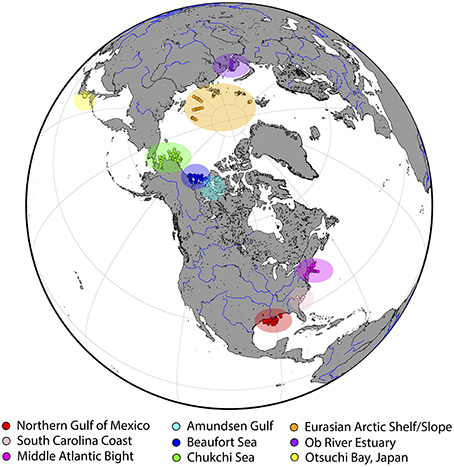
Figure 1. The nine ocean regions investigated in this study, along with their corresponding sampling sites. A total of 421 sample sets were collected between 2005 and 2013. Sampling details are provided in Table 1.

TABLE 1

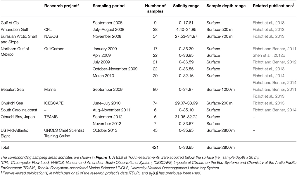
Table 1. General sampling information.

CDOM Sampling and Analysis

Most samples for CDOM analysis were gravity filtered from Niskin bottles using Whatman Polycap Aqueous Solution (AS) cartridges (0.2-μm pore size), collected in pre-combusted borosilicate glass vials, and stored immediately at 4°C until analysis in the laboratory. A few samples were collected using a bucket and filtered using a peristaltic pump through the Whatman Polycap Aqueous Solution (AS) cartridges. Absorbance of the samples was measured from λ = 250–800 nm using an ultraviolet (UV)-visible dual-beam spectrophotometer (Shimadzu UV-1601 or UV-2401PC/2501PC) and 10-cm quartz cells. For riverine and low-salinity samples (salinity < 10), 5-cm quartz cells or 1-cm quartz cuvettes were used. An exponential fit of the absorbance spectrum over an optimal spectral range was used to derive an offset value that was subtracted from the absorbance spectrum (Fichot and Benner, 2011). The optimal spectral range for the fit was typically 400–700 nm, but was adjusted for each sample (e.g., 350–700, 450–700 nm) as to provide the best fit of the absorbance spectrum possible over that spectral range. Absorbance corrected for offset was then converted to Napierian absorption coefficients, a_g(λ) (m⁻¹). The dependence of a_g(λ) on λ is described using Equation (1):

$\begin{array}{ll}{a}_g\left(\lambda \right)=a_g\left({\lambda }_0\right)·\text{exp}\left(-S\left(\lambda -{\lambda }_0\right)\right)& (1)\end{array}$

where λ₀ < λ and S is the spectral slope coefficient in the λ₀–λ nm spectral range. A careful examination of each a_g(λ) spectrum demonstrated the a_g(λ)-values (especially for λ > 350 nm) were well above the uncertainty of the measurement (±0.005 m⁻¹ at λ = 400 nm, for a 10-cm pathlength). The spectral slope coefficient of CDOM between 275 and 295 nm, S_275−295, was calculated as the slope of the linear regression of ln[a_g(λ)] on λ, between λ = 275 and 295 nm (Helms et al., 2008; Fichot and Benner, 2011). The S_275−295-values are reported in nm⁻¹.

Lignin Sampling and Analysis

Samples for lignin analysis (1–10 L) were gravity filtered from Niskin bottles using Whatman Polycap AS cartridges (0.2-μm pore size), acidified to pH = 2.5–3 with sulfuric acid, and extracted within a few hours using C-18 cartridges (Louchouarn et al., 2000). Cartridges were stored at 4°C until elution with 30 mL of methanol (HPLC-grade). The eluent was stored in sealed, pre-combusted glass vials at –20°C until analysis. Lignin phenols were analyzed using the CuO oxidation method of Kaiser and Benner (2012). Concentrations of lignin phenols were measured as trimethylsilyl derivatives using an Agilent 7890 gas chromatograph equipped with a Varian DB5-MS capillary column and an Agilent 5975 mass selective detector. The sum of nine lignin phenols was calculated as the total lignin phenol concentration: p-hydroxybenzaldehyde (PAL), p-hydroxyacetophenone (PON), p-hydroxybenzoic acid (PAD), vanillin (VAL), acetovanillone (VON), vanillic acid (VAD), syringaldehyde (SAL), acetosyringone (SON), and syringic acid (SAD). The sum of nine p-hydroxy, vanillyl, and syringyl lignin phenols is denoted as TDLP₉ and is reported in units of nmol L⁻¹. The sums of concentrations of the three p-hydroxy phenols (PAL+PON+PAD), three vanillyl phenols (VAL+VON+VAD), and three syringyl phenols (SAL+SON+SAD) were also calculated, and are denoted here as P, V, and S phenols. All values of P, V, and S phenols are reported in units of nmol L⁻¹. The P/V and S/V ratios were also calculated and are unitless.

Models

The models presented in this work for predicting dissolved lignin concentration from CDOM absorption coefficients were developed using the R environment for statistical computing and graphics and the “lm {stats}” function, obtained from the Comprehensive R Archive Network (https://cran.r-project.org).

Results and Discussion

The Relationship between Lignin and CDOM Absorption Coefficients Across Coastal Oceans

A strong, non-linear relationship between dissolved lignin concentrations and the ultraviolet (UV) absorption coefficients of CDOM was observed over the full range of lignin concentrations measured in this study (Figures 2A,C). Dissolved lignin concentrations, TDLP₉, ranged more than 500-fold from < 1 to 491 nmol L⁻¹, and the CDOM absorption coefficient, a_g(λ), ranged 85-fold at λ = 250 nm (1.1–84.5 m⁻¹), and 300-fold at λ = 400 nm (0.025–7.8 m⁻¹). The relationship between TDLP₉ and a_g(λ) followed a relatively well-behaved exponential over the wide range of lignin concentrations and coastal environments sampled, thereby indicating that the observed variations in CDOM UV absorption are tightly linked to changes in lignin along the river-ocean continuum (Figures 2A,C). The concave-down shape of the exponential (Figures 2A,C) further indicated that the rate of decrease of a_g(λ) relative to that of TDLP₉ (i.e., the derivative of the fitted line) increased substantially as lignin concentration decreased along the river-ocean continuum. At 250 nm, this rate increased about nine-fold from 0.09 to 0.75 L nmol⁻¹ m⁻¹, meaning a_g(250) decreased 9 times faster in high-salinity waters than in low-salinity waters for the same 1 nmol L⁻¹ decrease in TDLP₉ along the river-ocean continuum. The exponential behavior was less accentuated at 400 nm, for which the rate increased only 3-fold from ~0.01 to 0.035 L nmol⁻¹ m⁻¹.

FIGURE 2

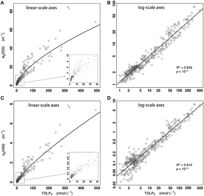
Figure 2. (A,B) Scatter plots of a_g(250) vs. TDLP₉ for the entire data set (n = 421) displayed using linear-scale and log-scale axes, respectively. The inset in (A) is a close-up of the relationship for the lower a_g(250) and TDLP₉-values. The coefficient of determination (R²) and p-value of the linear regression of ln[a_g(250)] on ln(TDLP₉) are shown in (B). (C,D) Same as (A,B) but for a_g(400).

Linear regressions of the form shown in Equation (2) provided adequate fits for the exponential relationship between TDLP₉ and a_g(λ) at any wavelength in the 250–400 nm range (Figures 2B,D, 3A).

$\begin{array}{ll}\text{ln}\left(a_g\left(\lambda \right)\right)=\alpha ·ln\left({\text{TDLP}}_9\right)+\beta & (2)\end{array}$

FIGURE 3

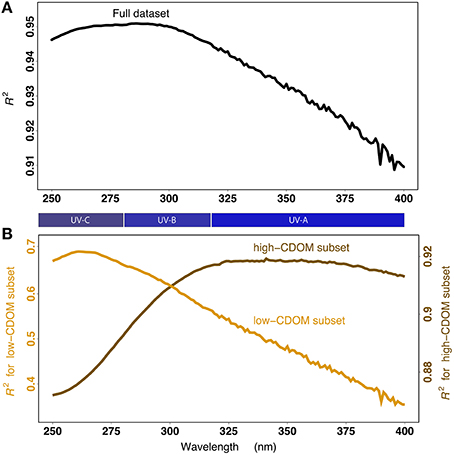
Figure 3. (A) Coefficient of determination (R²) of the linear regression of ln [a_g (λ)] on ln(TDLP₉) as a function of wavelength λ, and using the entire data set (n = 421). Note the regression lines corresponding to the R² at λ = 250 nm and 400 nm are shown in Figures 2B,D, respectively. (B) Same as in panel A but using a “low-CDOM” subset of the entire data set [a_g(250) < 4 m⁻¹; n = 263], shown here in orange, or a “high-CDOM” subset of the entire data set [a_g(250) ≥ 4 m⁻¹; n = 158], shown here in brown. The corresponding ranges of the UV-A, UV-B, and UV-C are shown for reference.

The relationship was stronger with a_g(250) than with a_g(400), as indicated by the coefficient of determination (R²) of Equation (2) decreasing from 0.946 at 250 nm to 0.910 at 400 nm (Figures 2B,D). A comparison of the R² for every wavelength between 250 and 400 nm further indicated the overall relationship was strongest (R² > 0.95) at ~285 nm (Figure 3A). Despite the goodness of the regression, significant scatter around the fitted lines was evident. A close examination of the relationship between TDLP₉ and a_g(250) using log-scale axes (Figure 2B) revealed that the scatter was relatively uniform (i.e., homoscedastic) over the entire range of lignin concentration. In contrast, the scatter around the fit was much less uniform (i.e., heteroscedastic) for a_g(400), and increased substantially and progressively with decreasing lignin concentration (Figure 2D). The linear relationship between TDLP₉ and a_g(400) was marginal (R² < 0.4) when lignin concentration was < 6 nmol L⁻¹.

The strength of the relationship between dissolved lignin concentration and CDOM absorption was maximal in the UV-C region at low lignin concentrations, and shifted to the UV-A region at higher lignin concentrations (Figure 3B). Additional insights about the relationship were gained by comparing the R² of Equation (2) for two subsets of the entire data set: 1) a “low-CDOM” subset (n = 263) where a_g(250) < 4 m⁻¹, and 2) a “high-CDOM” subset (n = 158) where a_g(250) ≥ 4 m⁻¹. The R² analysis using the “low-CDOM” subset (Figure 3B) revealed the relationship was optimal (R² ~ 0.7) at 250-275 nm (UV-C region), but weakened progressively and rapidly with wavelength to reach a minimal value (R² ~ 0.35) at 400 nm. The a_g(263) was the optimal predictor of TDLP₉ for the “low-CDOM” subset. However, the a_g(λ) in the UV-A region (λ > 320 nm) was generally a poor predictor of lignin concentration in waters less influenced by terrigenous inputs. Interestingly, the reverse trend was observed when examining the “high-CDOM” subset. The R² analysis using the “high-CDOM” subset (Figure 3B) indicated the relationship was good at all wavelengths, but improved significantly from a minimum R² = 0.87 at 250 nm to a R² ~ 0.92 in the UV-A region (320–400 nm). As will be explained later, this shift from UV-A to UV-C is likely related to the progressive change in the molecular structure of lignin, and potentially, of other terrigenous chromophores co-varying with lignin. This shift also indicates that a_g(λ) at a single wavelength is not an optimal predictor for lignin concentration over the range of lignin concentration found in coastal oceans.

The p-hydroxy phenols (P), vanillyl phenols (V), and syringyl phenols (S) that make up TDLP₉ exhibited varying degrees of correlation with the CDOM absorption coefficient (Figure 4). As explained earlier, the relationship between a_g(λ) and TDLP₉ was optimal at ~285 nm for the entire range of lignin concentrations (R² = 0.951). The separation of TDLP₉ into P, V, and S phenols indicated the relationship between a_g(285) and P phenols across the full range of values was even stronger (R² = 0.959) than with TDLP₉. Only samples from the Ob estuary deviated significantly from the general relationship, and were enriched in P phenols relative to a_g(285). However, this enrichment in P phenols was apparent and most likely originated from elevated levels of peat-derived sphagnum acid typically found in the Ob watershed, and their subsequent conversion into P phenols during the oxidation of lignin (Amon et al., 2012; Philben et al., 2014). The relationship became progressively less robust with V phenols (R² > 0.925) and S phenols (R² > 0.893). The trend is consistent with P phenols being more resistant to degradation in natural waters than V phenols, and with S phenols being the most susceptible to degradation (Opsahl and Benner, 1995; Benner and Opsahl, 2001; Benner and Kaiser, 2011). Furthermore, lignin produced by gymnosperms is devoid of S phenols, whereas P and V phenols are ubiquitous in lignin (Hedges and Mann, 1979; Benner and Opsahl, 2001; Shen et al., 2012b). This most likely impacted the relationship between a_g(285) and S phenols by making it sensitive to variations in watershed vegetation.

FIGURE 4

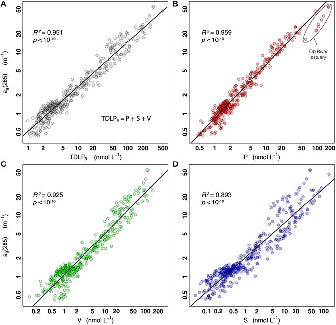
Figure 4. Relationships between a_g(285) and the concentrations of (A) TDLP₉, (B) p-hydroxy phenols, (C) vanillyl phenols, (D) and syringyl phenols.

Physical Mixing and Degradation Of Terrigenous CDOM

The decreasing trends in TDLP₉ concentrations and a_g(285) along the salinity gradient confirmed the importance of physical mixing in the distribution of these two variables along the river-ocean continuum (Figure 5). As expected from the strong relationship observed between TDLP₉ and ag(285), the relationships between salinity and TDLP₉ (Figures 5A,B) and between salinity and a_g(285) (Figures 5C,D) were strikingly similar. Although a large scatter in TDLP₉ and a_g(285) at salinities < 5 and >35 indicated important differences among riverine sources and ocean end-members, the trends observed for each region clearly indicated physical mixing of riverine and oceanic end-members played a dominant role in regulating the variability of TDLP₉ and a_g(285) concentrations. Two South Carolina samples strongly influenced by salt-marsh inputs (Ashley River and Hunting Island, SC) stood out as being relatively enriched in CDOM and lignin, in agreement with previous observations that marsh-derived CDOM can be chemically and optically distinct (e.g., stronger absorption) from other estuarine CDOM (Tzortziou et al., 2008). In contrast, samples with salinities ~28–33 from the Western Arctic Ocean (Chukchi Sea, Beaufort Sea, Amundsen Gulf) stood out as being relatively depleted in CDOM and lignin. Considering most of these samples were collected in regions experiencing extensive sea-ice melting, this relative depletion in CDOM and lignin was likely due to the presence of ice-melt water (low salinity and depleted in DOM).

FIGURE 5

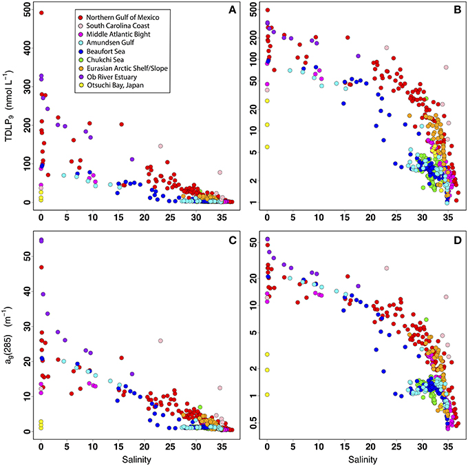
Figure 5. Relationships between salinity and TDLP₉ using a linear-scale y-axis (A) and a log-scale y-axis (B), and relationships between salinity and a_g(285) using a linear-scale y-axis (C) and a log-scale y-axis (D).

Several degradation indicators further indicated the general decrease in lignin concentrations from the rivers to the oligotrophic regions of coastal oceans was accompanied by a progressive change in the degradation state of terrigenous CDOM (Figure 6). The TDLP₉-values decreased by almost four orders-of-magnitude along the river-ocean continuum. This decrease exhibited a weak, but significant and positive correlation (r = 0.51) with the ratio of S to V phenols (S/V), and was accompanied by exponential increases in the ratio of P to V phenols (P/V) and the spectral slope coefficient of CDOM absorption (S_275−295). These trends are consistent with similar observations along the salinity gradient of river-influenced ocean margins in previous studies, and with the physical mixing of two terrigenous CDOM end-members with different degradation states (Opsahl and Benner, 1998; Hernes and Benner, 2003; Helms et al., 2008; Fichot and Benner, 2012).

FIGURE 6

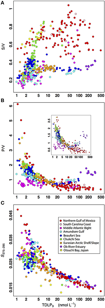
Figure 6. Relationships between TDLP₉ and several degradation indicators of lignin and CDOM degradation: (A) S/V ratio of syringyl phenols to vanillyl phenols (unitless), (B) P/V ratio of p-hydroxy phenols to vanillyl phenols (unitless), and (C) the spectral slope coefficient of CDOM absorption coefficient spectrum between 275 and 295 nm, S_275−295 (nm⁻¹).

More specifically, the trends in S/V, P/V, and S_275−295 observed herein are consistent with the physical mixing of two end-members: (1) a relatively unaltered terrigenous CDOM end-member from rivers, and (2) a photochemically altered terrigenous CDOM end-member from the oligotrophic regions of the coastal oceans (Benner and Opsahl, 2001; Hernes and Benner, 2003; Fichot and Benner, 2012). The S/V has been shown to decrease during natural sunlight photodegradation experiments and during coupled photochemical-biological degradation experiments under simulated sunlight (Opsahl and Benner, 1998; Spencer et al., 2009; Benner and Kaiser, 2011). Note that Spencer et al. (2009) actually showed an increase in S/V after extreme exposure to solar radiation, but only after an initial decrease in S/V. The P/V has also been shown to increase during photodegradation experiments (Benner and Kaiser, 2011). In addition, the S_275−295 has been shown to increase with decreasing molecular weight of CDOM and during exposure to solar radiation (Helms et al., 2008; Fichot and Benner, 2012; Yamashita et al., 2013). The trends in S/V, P/V, and S_275−295 observed in this data set are consistent with the effects of photodegradation, and suggest the progressive change in the degradation state of terrigenous CDOM played an important role shaping the relationship between lignin and CDOM absorption coefficients.

The relatively weak correlation (r = 0.51) between the S/V and TDLP₉ was not unexpected (Figure 6A). The S/V is not only affected by solar exposure, but is also a well-established indicator of the source vegetation of lignin and terrigenous DOM in natural waters (Hedges and Mann, 1979; Hedges and Ertel, 1982; Opsahl et al., 1999; Dittmar and Kattner, 2003; Shen et al., 2012b). As mentioned earlier, the S/V reflects the relative contributions of gymnosperm and angiosperm vegetation in lignin and terrigenous DOM because S phenols are not produced by gymnosperms. Lower S/V are thus typically measured in lignin that originates from gymnosperm-dominated watersheds (e.g., boreal forests), whereas higher S/V are indicative of significant contributions from angiosperms (e.g., tundra, deciduous forests). The effect of vegetation source on lignin phenol composition was evident in this data set, with low S/V values (< 0.5) measured in Arctic waters. The drainage basins of large Arctic rivers are dominated by gymnosperms, and the S/V of Arctic rivers typically range from ~0.2 to 0.45 (when calculated from nmol L⁻¹ concentrations) and exhibit some moderate variations with flow regime (Amon et al., 2012). The effect of vegetation was also evident from the high S/V values (>0.5) measured in the sub-tropical and temperate coastal oceans, which receive substantial contributions from angiosperms. Some samples from the Chukchi Sea had relatively high S/V values, but these samples were strongly influenced by Pacific Ocean water or small rivers draining tundra. Finally, a large number of samples from the Middle Atlantic Bight had comparatively low S/V values. This was likely observed because most of the terrigenous DOM on the shelf of the Middle Atlantic Bight shelf originates from gymnosperm-dominated environments further north, and is transported southward by currents (Chapman and Beardsley, 1989; Mountain, 1991).

Evidence suggests the P/V ratio is a useful indicator of the extent of lignin degradation. Here, the P/V increased several-fold and exponentially with decreasing lignin concentrations (Figure 6B). The P/V has been shown to increase substantially after continuous or intermittent solar exposure (Benner and Kaiser, 2011), and unlike the S/V, the P/V is not as sensitive to changes in source vegetation. The P phenols are widely distributed among vascular plants. However, as mentioned earlier, inputs from peatlands can increase the P/V, most likely as a result of the conversion of sphagnum acid into P phenols during CuO oxidation. Elevated concentrations of P phenols were observed in the peatland-influenced samples from the Ob River estuary, and to a much lesser degree, from the Mackenzie River estuary. Samples influenced by sub-tropical salt marshes (e.g., Terrebonne Bay, South Carolina Coast) also have slightly elevated values of P/V. Note the P/V can also reflect changes in the flow regime of rivers and be indicative of the ¹⁴C age of terrigenous DOM immobilized (Amon et al., 2012). High P/V and lower lignin concentrations have thus been observed during base flow in Arctic Rivers, and the reverse observed during peak flow (Amon et al., 2012), suggesting that changes in river flow could contribute to the trends observed here between TDLP₉ and P/V. Finally, the highest P/V-values (>4) were observed in samples from oligotrophic eddies shed from the Loop Current and impinging on the continental shelf in the northern Gulf of Mexico (Schiller et al., 2011; Fichot et al., 2014). These high P/V were likely attributed to the long-term solar exposure and degradation in the optically clear Loop-Current waters, which originate in the Atlantic Ocean.

The exponential increase in S_275−295 with decreasing lignin concentrations was also consistent with physical mixing and the effects of photochemical degradation (Figure 6C). S_275−295 has been shown to increase during photodegradation and is a sensitive indicator of CDOM photodegradation in natural waters (Helms et al., 2008, 2013; Ortega-Retuerta et al., 2009; Fichot and Benner, 2012; Yamashita et al., 2013). Overall, the S_275−295 displayed a clear increasing trend with decreasing TDLP₉ concentrations in the present study. With the exception of a few outliers, S_275−295 increased monotonically with decreasing TDLP₉-values ranging from 500 to 10 nmol L⁻¹. When TDLP₉ was < 10 nmol L⁻¹, the relationship between S_275−295 and TDLP₉ split into two groups of data: one that continued to show a strong relationship between S_275−295 and TDLP₉, and one that showed little correlation between the two. The first group consisted essentially of surface samples, whereas the second group corresponded primarily of sub-surface and deep waters, and of productive, high-latitude waters that were moderately influenced by terrigenous inputs (e.g., Chukchi Sea, Canada Basin, Amundsen Gulf). Limited solar exposure, a greater relative contribution of microbial degradation, or a more prominent influence of non-terrigenous sources of CDOM (in situ production) can be expected in these water types, and are consistent with the relatively low S_275−295-values (~0.025 nm⁻¹) observed. The limited solar exposure in sub-surface and deep water likely contributed to the lower S_275−295. Furthermore, previous studies reported S_275−295-values of ~0.025 nm⁻¹ for plankton-derived CDOM, and have provided evidence that S_275−295 decreases slightly during microbial degradation (Ortega-Retuerta et al., 2009; Fichot and Benner, 2012).

It is important to understand that the progressive changes in the degradation state of terrigenous CDOM observed along the river-ocean continuum are largely driven by the physical mixing of riverine and ocean end-members (Fichot and Benner, 2012), and that the observed change largely reflects long-term effects of photochemical degradation on the ocean end-member of terrigenous CDOM. Terrigenous CDOM, which remains relatively unaltered in rivers, mixes with photochemically altered terrigenous CDOM from oligotrophic regions of ocean margins (Benner and Opsahl, 2001; Hernes and Benner, 2003; Fichot and Benner, 2012). Solar exposure in surface waters and the extent of photochemical degradation occurring over typical residence times of river water in ocean margins (e.g., months) has been shown to be relatively moderate, even in subtropical river-influenced ocean margins (Fichot and Benner, 2014). Much of the photochemical degradation occurs beyond the shelf where the residence time of the water is much longer and solar exposure in surface waters is strongly enhanced by a sharp increase in UV penetration relative to the mixed layer depth. In some cases, the terrigenous CDOM found in the oligotrophic regions of the coastal oceans can have a very different and more distant origin, as was the case in this data set when Loop-Current oligotrophic eddies impinged on the Northern Gulf of Mexico shelf (Fichot et al., 2014). In the Arctic Ocean, solar exposure and photodegradation are less than in subtropical regions, but the ocean end-member can have a more distant origin and the terrigenous CDOM can be more chemically altered (e.g., Pacific Water in Chukchi or Beaufort Seas, or Atlantic water off Svalbard).

The concave-down shape of the exponential relationship between TDLP₉ and a_g(λ) was consistent with mixing and long-term photodegradation playing important roles in shaping the relationship between lignin concentration and CDOM absorption coefficients. Photodegradation has been shown to lead to a decrease in the molecular weight and aromaticity of terrigenous CDOM (Kieber et al., 1989, 1990; Opsahl and Benner, 1998; Miller et al., 2002; Helms et al., 2008). The molecular weight and aromaticity of a compound is, in turn, strongly linked to its molar absorptivity (Chin et al., 1994; Weishaar and Aiken, 2001), such that a given concentration of lignin in low-molecular-weight molecules absorbs much less efficiently than the same concentration of lignin within high-molecular weight molecules. The concave-down shape of the relationship indicated there was an acceleration in the loss of a_g(λ) relative to that of TDLP₉ as lignin concentrations decreased from riverine to oligotrophic waters. A loss of absorption strictly due to the loss of chromophoric material (i.e., without a loss of molar absorptivity) would tend to produce a linear rather than a concave-down exponential relationship. Here, the acceleration in the loss of a_g(λ) was consistent with a progressive loss of molar absorptivity superimposed on a loss of chromophoric material, and is consistent with previous observations of a decrease in molecular weight of both CDOM and lignin along the river-ocean continuum in ocean margins (Hernes and Benner, 2003; Helms et al., 2008).

The characteristics of the relationship between TDLP₉ and a_g(400) were consistent with a progressive loss of intramolecular charge-transfer interactions in CDOM along the river-ocean continuum. Intramolecular charge-transfer interactions among chromophores in aromatic molecules such as lignin have been proposed as a mechanism to explain the exponential shape of the CDOM absorption spectrum and its absorption at wavelengths >350 nm (Del Vecchio and Blough, 2004; Boyle et al., 2009; Sharpless and Blough, 2014). In this model, charge-transfer interactions among electron donors (e.g., phenols and/or methoxylated phenols in lignin) and electron acceptors (e.g., quinones or aromatic ketones/aldehydes in lignin) are thought to produce lower-energy optical transitions and enhance CDOM absorption at wavelengths >350 nm. The contribution of electronic interactions to the CDOM absorption is linked to the molecular weight of terrigenous molecules like lignin, because compounds with higher molecular weight have a greater potential for intramolecular charge-transfer interactions. A sharp decrease in the molecular weight of lignin along the river-ocean continuum would therefore be associated with a loss of intramolecular charge-transfer interactions, and with a weakening contribution of lignin to the CDOM absorption at wavelengths >350 nm. The worsening of the relationship between TDLP₉ and a_g(400) with decreasing lignin concentrations, which eventually leads to an insignificant relationship between TDLP₉ and a_g(400) in the more oligotrophic regions of the coastal oceans, is consistent with the effects of photodegradation.

On the Contribution of Lignin and other Components to CDOM Absorption

The existence of a well-behaved relationship between TDLP₉ and a_g(λ) from the rivers to the oligotrophic regions of several contrasting coastal oceans was a strong indication that lignin is generally an important driver of the variability of CDOM absorption coefficients in coastal waters. However, the contribution of lignin to the absorption coefficient of CDOM was not uniform across the 250–400 nm spectrum. Lignin appeared an important contributor to a_g(λ) in the UV-C (λ < 280 nm) and UV-B (280 < λ < 320 nm) regions over the entire range of lignin concentrations observed in this study. However, for λ> 350 nm, lignin only seemed to contribute significantly to CDOM absorption for the upper range of TDLP₉ concentrations and a_g(λ) values (e.g., TDLP₉ > 10 nmol L⁻¹ or a_g(250) > 4 m⁻¹). For this upper range, lignin appeared an even greater contributor to a_g(λ) in the UV-A region than in the UV-B and UV-C regions. As described earlier, the spectral dependency of the relationship likely results from the change in the degradation state of terrigenous CDOM. The P phenols in lignin appeared to be the greater contributor to the absorption coefficients of CDOM, followed by the V phenols and the S phenols. A greater contribution of the P phenols to CDOM absorption is consistent with their greater resistance to photodegradation (Benner and Kaiser, 2011), and their selective preservation relative to the V and S phenols as lignin concentrations decrease along the river-ocean continuum. Although this is only speculation, it is possible the greater photochemical resistance of P phenols contributes to their preservation in higher molecular weight and more aromatic structures that have higher molar absorptivities and higher potential for intramolecular electronic interactions. The selective preservation of the P phenols is consistent with the strong relationship observed between P phenols and a_g(λ) in the more oligotrophic regions of the coastal oceans.

A variety of other chromophoric constituents in terrigenous DOM also likely contribute to CDOM absorption and impact the relationship between lignin and CDOM. Lignin has the chemical moieties necessary to make it an important chromophore (Boyle et al., 2009; Sharpless and Blough, 2014). It is important to recognize, however, that a variety of other chromophoric components in terrigenous DOM likely co-vary strongly with lignin, and can contribute significantly to the CDOM absorption despite the strong linkage observed between CDOM and lignin. Tannins, a class of polyphenols, are components of many terrestrial plant tissues (e.g., foliage, bark) and are readily released to aquatic systems (Benner et al., 1990; Hernes et al., 2001; Kraus et al., 2003; Maie et al., 2008). Dissolved tannins also absorb very strongly in the ultraviolet and visible region (Lawrence, 1980; Alberts, 1982; Kraus et al., 2003). However, previous studies have reported that tannin concentrations are very low in natural waters (Maie et al., 2006), and that microbial degradation, precipitation, sorption to sediments and potentially photodegradation removes tannins from aquatic systems (Benner et al., 1986; Hernes et al., 2001; Maie et al., 2008). The contribution of tannins to the CDOM absorption in coastal waters remains unclear, and more work is needed to directly assess the linkage between tannins and CDOM in coastal oceans.

Dissolved black carbon is a component of terrigenous DOM, and several studies indicate it is a potentially important component of DOC in natural waters (Kim et al., 2004; Mannino and Harvey, 2004; Ziolkowski and Druffel, 2010; Dittmar et al., 2012). Dissolved black carbon is thought to contribute up to 10% of the global riverine DOC flux to the ocean (Jaffé et al., 2013), and it contains condensed aromatic compounds that absorb strongly in the ultraviolet region (Russo et al., 2012). Stubbins et al. (2015) showed that dissolved black carbon concentration was more strongly correlated with a_g(250) than with a_g(400) for high-CDOM samples [a_g(250)~10–150 m⁻¹]. Interestingly, our study revealed the reverse trend for lignin, with lignin concentration being more strongly correlated with a_g(400) than with a_g(250) for samples from a similar range of CDOM absorption [a_g(250) ~ 4–100 m⁻¹]. These opposing trends are possibly linked to differences in the molecular structures of dissolved black carbon and dissolved lignin. Black carbon contains condensed aromatic compounds that typically have very high molar absorptivities in the UV (Chin et al., 1994; Weishaar and Aiken, 2001; Russo et al., 2012), whereas partially oxidized lignin contains the moieties responsible for intramolecular charge-transfer interactions, which are particularly effective at absorbing at wavelengths >350 nm (Del Vecchio and Blough, 2004; Boyle et al., 2009; Sharpless and Blough, 2014). Soils are a major source of black carbon and lignin, suggesting these two components likely correlate strongly in river-influenced coastal areas. More work is needed to better understand the potential contribution of black carbon to the optical properties of CDOM along the river-ocean continuum.

An analysis of the percent residuals from the linear fit of the a_g(285)–TDLP₉ relationship revealed some interesting variations among the different coastal oceans of this study (Figures 7, 8). Although deviations from the fitted line can occur for a variety of reasons, independent variations in the relative contributions of other, non-lignin components are likely a dominant factor. Plankton and microbes can also produce chromophoric compounds (e.g., amino acids, nucleic acids) that have variable effects on the CDOM dynamics of natural waters and will tend to contribute to the scatter in the relationship between TDLP₉ and a_g(λ) (Rochelle-Newall and Fisher, 2002; Nelson et al., 2004; Yamashita and Tanoue, 2008; Ortega-Retuerta et al., 2009; Zhang et al., 2009; Fichot and Benner, 2012). Most of the samples from the Northern Gulf of Mexico, Middle Atlantic Bight, Eurasian shelf, and Otsuchi Bay, exhibited elevated TDLP₉-values relative to a_g(285) (i.e., negative residuals), thereby suggesting lignin was a more dominant contributor to a_g(285) in these waters. The deviation was particularly strong in the Otsuchi Bay waters, which receives inputs from short and steep rivers with short water residence times. In contrast, most samples from the Amundsen Gulf, Beaufort Sea, Chukchi Sea, Ob estuary, and South Carolina coast exhibited relatively low TDLP₉-values compared to a_g(285) (i.e., positive residuals), suggesting a greater contribution of non-lignin chromophores. The positive residuals in the Chukchi Sea (all collected in summer) were potentially related to a higher background of autochthonous CDOM in these productive waters (Shen et al., 2012a), whereas those of the Ob estuary are consistent with significant contribution of non-lignin CDOM from Sphagnum sp. peats (Amon et al., 2012; Philben et al., 2014). The positive residuals in the South Carolina coast samples are likely related to contributions from the tidal marshes, which have been shown to have distinctive CDOM chemical and optical properties (Tzortziou et al., 2008). Finally, many of the positive residuals were from samples collected in or near rivers during summer, and could be related to the in situ production of CDOM, or be related to depletion of lignin observed after the peak river flow during spring (Amon et al., 2012; Shen et al., 2012b).

FIGURE 7

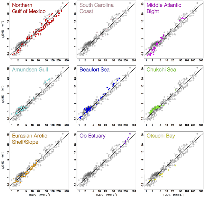
Figure 7. Scatter plots of the relationship between a_g(285) and TDLP₉ (log-scale axes) highlighting the data from each of the nine study regions.

FIGURE 8

Figure 8. Boxplots showing the distribution of the percent residual from the linear regression of ln[a_g(285)] on ln(TDLP₉) for each of the nine study regions. The dashed gray line at 0% corresponds to the linear fit. Each boxplot indicates how the data from each region deviate from the general relationship between lignin and a_g(285).

Empirical Models for Estimating TDLP₉ from a_g(λ)

Exploration of lignin and CDOM relationships provided useful information for the development of two simple empirical models for the retrieval of TDLP₉ from a_g(λ) in coastal oceans. The a_g(285) was, on average, the best single-wavelength predictor of TDLP₉ over the range of absorption coefficients and lignin concentrations observed in this study. However, the spectral dependency of the relationship indicated a_g(263) was the optimal single-wavelength predictor of TDLP₉ for samples where a_g(250) < 4 m⁻¹, and a_g(350) was the optimal single-wavelength predictor for TDLP₉ for samples where a_g(250) ≥ 4 m⁻¹. Furthermore, photodegradation had a strong effect on the relationship, and S_275−295 helped factor in this effect and improve the TDLP₉ predictions for high-CDOM samples, where S_275−295 and TDLP₉ were most correlated [TDLP₉ ≥ 10 nmol L⁻¹ or a_g(250) ≥ 4 m⁻¹]. These observations guided the development of two sub-models separated by the a_g(250) = 4 m⁻¹ cutoff.

When a_g(250) < 4 m⁻¹, a “low-CDOM” sub-model based on a simple linear regression was used,

$\begin{array}{ll}\text{ln}\left({\text{TDLP}}_9\right)=0.7672·a_g\left(263\right)-0.3987& (3)\end{array}$

When a_g(250) ≥ 4 m⁻¹, a “high-CDOM” sub-model based on a multiple linear regression was used,

$\begin{array}{l}\text{ln}\left({\text{TDLP}}_9\right)=-2.282·\text{ln}\left(a_g\left(350\right)\right)-8.209·\text{ln}\left(a_g\left(275\right)\right)\\ +11.365·\text{ln}\left(a_g\left(295\right)\right)+2.909& (4)\end{array}$

In the case of the multiple linear regression of Equation (4), all derived coefficients were significant by the t-test (p < 0.0005), thereby confirming a_g(275) and a_g(295) represented meaningful additions to the model. The addition of a_g(275) and a_g(295) also improved the adjusted R² of the regression (adj R² = 0.936) relative to a single regression model using only a_g(350) (adj R² = 0.918). The use of a_g(275) and a_g(295) in Equation (4) was somewhat similar to using S_275−295 as one of the terms, but did not require the extra step of calculating S_275−295. Note the use of additional predictors in either Equation (3) or (4), or the use of partial-least-square regressions did not significantly improve the adjusted R² of the regressions nor the % error of the estimates relative to these simple empirical models. This indicated the useful information contained in the spectral shape of CDOM was mostly exploited. Note here, that even though the predictor terms in Equation (4) are strongly correlated, multi-collinearity does not represent an issue for predictive models. Multi-collinearity is problematic when trying to interpret the meaning of the derived parameters in the equations.

Overall, these simple empirical models provide a practical means to derive reasonably accurate estimates of TDLP₉ from CDOM absorption coefficients in coastal oceans (Figures 9, 10). A comparison of the measured and estimated TDLP₉ indicated the model retrieved TDLP₉-values that were on average within ±20% of the measured values (Figure 9). The % error was < 17% for half of all retrieved TDLP₉-values, and it very rarely exceeded 60%. As it is currently parameterized, the model might slightly underestimate some of the very high lignin concentrations found in rivers (>200 nmol L⁻¹). The capacity of the model to reproduce realistic distributions of TDLP₉ was also assessed for a cross-shelf section of the Middle Atlantic Bight (Figure 10). This subset of the data set was chosen because it encompassed a coastal region with a moderate gradient in TDLP₉, and included data from both surface and sub-surface waters. The model adequately reproduced the most important features of the measured-TDLP₉ distribution along the salinity gradient. For instance, the cross-shelf gradient from the lignin-rich mouth of the Hudson River to the depleted open waters of the Middle Atlantic Bight was well-reproduced, just like the subsurface TDLP₉ maximum measured at the entrance of Hudson canyon. The more subtle features of the TDLP₉ distribution were less well-reproduced. The average error of ±20% associated with the retrievals implies that the model can only reproduce significant gradients in lignin.

FIGURE 9

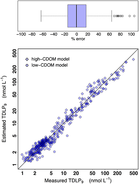
Figure 9. Performance overview of dissolved-lignin-concentration prediction models proposed in this study. Two separate models are used to predict TDLP₉ from a_g(λ), and the cutoff a_g(250) = 4 m⁻¹ is used to separate the two models. For the low-CDOM model where a_g(250) < 4 m⁻¹, a simple linear regression between a_g(263) and TDLP₉ is used. In contrast, a multiple-linear-regression model of ln(TDLP₉) on ln[a_g(λ)] (λ = 275, 295, and 350 nm) is used for the high-CDOM model when a_g(250) ≥ 4 m⁻¹. The parameters used to implement the models are provided in Equations (3) and (4).

FIGURE 10

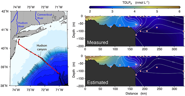
Figure 10. Comparison of the measured distribution of TDLP₉ to that predicted from a_g(λ) using the proposed models [Figure 9 and Equations (3) and (4)] along a cross-shelf transect in the Middle Atlantic Bight. The white contour lines shown in the cross-shelf sections correspond to salinity.

The model is expected to perform similarly well in most river-influenced coastal oceans of the world, as long as the TDLP₉ predictions are made within the ranges of a_g(λ) and TDLP₉-values used to train the model. The variety of coastal environments represented in this data set suggests the model will be suitable for most sub-tropical, temperate, and Arctic coastal oceans that receive notable inputs of terrigenous DOM. However, the performance of the model remains uncertain in coastal regions influenced by tropical rivers, as these were not represented in the training data set. More importantly, the use of the model is not recommended in major coastal upwelling systems that typically receive little terrigenous DOM inputs (e.g., California current, Benguela current). In these coastal water types, autochthonous sources of DOM are likely to exert a more dominant control on the dynamics of a_g(λ), and the link between TDLP₉ and a_g(λ) is likely to deviate significantly from the relationship established. Naturally, this simple model is not final, and can be very easily re-trained to improve and expand its applicability as more data become available.

Author Contributions

CF, RB, KK, CL, and HO collected the in situ samples for CDOM and lignin analysis. CF, KK, YS, and CL processed the lignin samples, and CF, YS, CL, and RA processed the CDOM samples. CF wrote the manuscript with important discussion with RB, KK, YS, and RA and with comments from all authors.

Conflict of Interest Statement

The authors declare that the research was conducted in the absence of any commercial or financial relationships that could be construed as a potential conflict of interest.

Acknowledgments

Most of the data used in this study were collected during research cruises carried out as part of the following projects: (1) the Malina Scientific Program (http://malina.obs-vlfr.fr) funded by ANR (Agence nationale de la recherche), INSU-CNRS (Institut national des sciences de l'univers, Centre national de la recherche scientifique), CNES (Centre national d'études spatiales), and ESA (European Space Agency); (2) the Circumpolar Flaw Lead (CFL) study (http://www.ipy-api.gc.ca/pg_IPYAPI_029-eng.html) funded by the Government of Canada (IPY #96); (3) the Impacts of Climate on the Eco-Systems and Chemistry of the Arctic Pacific Environment (ICESCAPE) program (http://www.espo.nasa.gov/icescape/) funded by NASA (National Aeronautics and Space Administration); (4) the Nansen and Amundsen Basin Observational System (NABOS) project (http://nabos.iarc.uaf.edu/index.php) funded by the US-NSF (National Science Foundation), NOAA (National Oceanographic and Atmospheric Administration), the ONR (Office of Naval Research), and JAMSTEC (Japan Marine Science and Technology Center), (5) the GulfCarbon project funded by the National Science Foundation (http://ocean.otr.usm.edu/~w301130/research/gulfcarbon_new.htm), and (6) the University-National Oceanographic Laboratory System (UNOLS) 2013 chief scientist training cruise sponsored by the National Science Foundation (https://www.unols.org/chief-scientist-training-cruise) and supported under NSF grant OCE-1230900. The Otsuchi Bay samples were collected as part of the research program “Tohoku Ecosystem-Associated Marine Sciences” (TEAMS) of the Ministry of Education, Culture, Sports, Science and Technology (MEXT). This work was directly supported by NSF grants 0713915 and 0850653 to R.B., and NSF grants 0229302, 0425582, 0713991 to R.M.W.A. We thank the following people: the crews of the R/V Cape Hatteras, R/V Hugh Sharp, R/V Endeavor, USCGC Healy, CCGS Amundsen, and Russian icebreaker Kapitan Dranitsyn for assistance with sample collection, Dr. Jolynn Carroll for collecting the Gulf-of-Ob samples, Stephanie Smith and Sally Walker for absorbance measurements on the NABOS samples, and Steven E. Lohrenz and Wei-Jun Cai for providing berths on the GulfCarbon cruises.

References

Aiken, G. R., and Cotsaris, E. (1995). Soil and Hydrology: their effects on NOM. J. Am. Water Work. Assoc. 87, 36–45.

Google Scholar

Aiken, G. R., McKnight, D. M., Wershaw, R. L., and MacCarthy, P. (eds.). (1985). “Humic substances,” in Soil, Sediment, and Water: Geochemistry, Isolation and Characterization (New York, NY: John Wiley & Sons), 363–385.

PubMed Abstract | Google Scholar

Alberts, J. J. (1982). The effect of metal ions on the ultraviolet spectra of humic acid, tannic acid and lignosulfonic acid. Water Res. 16, 1273–1276. doi: 10.1016/0043-1354(82)90146-4

CrossRef Full Text | Google Scholar

Amon, R. M. W., Rinehart, A. J., Duan, S., Louchouarn, P., Prokushkin, A., Guggenberger, G., et al. (2012). Dissolved organic matter sources in large Arctic rivers. Geochim. Cosmochim. Acta 94, 217–237. doi: 10.1016/j.gca.2012.07.015

CrossRef Full Text | Google Scholar

Benner, R., Hatcher, P. G., and Hedges, J. I. (1990). Early diagenesis of mangrove leaves in a tropical estuary: bulk chemical characterization using solid-state 13C NMR and elemental analyses. Geochim. Cosmochim. Acta 54, 2003–2013. doi: 10.1016/0016-7037(90)90268-P

CrossRef Full Text | Google Scholar

Benner, R., and Kaiser, K. (2011). Biological and photochemical transformations of amino acids and lignin phenols in riverine dissolved organic matter. Biogeochemistry 102, 209–222. doi: 10.1007/s10533-010-9435-4

CrossRef Full Text | Google Scholar

Benner, R., and Opsahl, S. (2001). Molecular indicators of the sources and transformations of dissolved organic matter in the Mississippi river plume. Org. Geochem. 32, 597–611. doi: 10.1016/S0146-6380(00)00197-2

CrossRef Full Text | Google Scholar

Benner, R., Peele, E. R., and Hodson, R. E. (1986). Microbial utilization of dissolved organic matter from leaves of the red mangrove, Rhizophora mangle, in the Fresh Creek estuary, Bahamas. Estuar. Coast. Shelf Sci. 23, 607–619. doi: 10.1016/0272-7714(86)90102-2

CrossRef Full Text | Google Scholar

Boyle, E. S., Guerriero, N., Thiallet, A., Del Vecchio, R., and Blough, N. V. (2009). Optical properties of humic substances and CDOM: relation to structure. Environ. Sci. Technol. 43, 2262–2268. doi: 10.1021/es803264g

PubMed Abstract | CrossRef Full Text | Google Scholar

Chapman, D. C., and Beardsley, R. C. (1989). On the origin of shelf water in the Middle Atlantic Bight. J. Phys. Oceanogr. 19, 384–391.

Google Scholar

Chin, Y., Aiken, G., and O'Loughlin, E. (1994). Molecular weight, polydispersity, and spectroscopic properties of aquatic humic substances. Environ. Sci. Technol. 28, 1853–1858.

PubMed Abstract | Google Scholar

Cota, G. F., Pomeroy, L. R., Harrison, W. G., Jones, E. P., Peters, F., Sheldon, W. M., et al. (1996). Nutrients, primary production and microbial heterotrophy in the southeastern Chukchi Sea: Arctic summer nutrient depletion and heterotrophy. Mar. Ecol. Prog. Ser. 135, 247–258. doi: 10.3354/meps135247

CrossRef Full Text

Del Vecchio, R., and Blough, N. V. (2004). On the origin of the optical properties of humic substances. Environ. Sci. Technol. 38, 3885–3891. doi: 10.1021/es049912h

PubMed Abstract | CrossRef Full Text | Google Scholar

Dittmar, T., de Rezende, C. E., Manecki, M., Niggemann, J., Coelho Ovalle, A. R., Stubbins, A., et al. (2012). Continuous flux of dissolved black carbon from a vanished tropical forest biome. Nat. Geosci. 5, 618–622. doi: 10.1038/ngeo1541

CrossRef Full Text | Google Scholar

Dittmar, T., and Kattner, G. (2003). The biogeochemistry of the river and shelf ecosystem of the Arctic Ocean: a review. Mar. Chem. 83, 103–120. doi: 10.1016/S0304-4203(03)00105-1

CrossRef Full Text | Google Scholar

Eriksson, K.-E. (2010). “Lignin Biodegradation,” in Lignin and Lignans, eds C. Heitner, D. R. Dimmel, and J. A. Schmidt (Boca Raton, FL: CRC Press), 495–520.

Fichot, C. G., and Benner, R. (2011). A novel method to estimate DOC concentrations from CDOM absorption coefficients in coastal waters. Geophys. Res. Lett. 38:L03610. doi: 10.1029/2010gl046152

CrossRef Full Text | Google Scholar

Fichot, C. G., and Benner, R. (2012). The spectral slope coefficient of chromophoric dissolved organic matter (S275–S295) as a tracer of terrigenous dissolved organic carbon in river-influenced ocean margins. Limnol. Oceanogr. 57, 1453–1466. doi: 10.4319/lo.2012.57.5.1453

CrossRef Full Text | Google Scholar

Fichot, C. G., and Benner, R. (2014). The fate of terrigenous dissolved organic carbon in a river-influenced ocean margin. Global Biogeochem. Cycles 28, 300–318. doi: 10.1002/2013GB004670

CrossRef Full Text | Google Scholar

Fichot, C. G., Kaiser, K., Hooker, S. B., Amon, R. M. W., Babin, M., Bélanger, S., et al. (2013). Pan-Arctic distributions of continental runoff in the Arctic Ocean. Sci. Rep. 3, 1053. doi: 10.1038/srep01053

PubMed Abstract | CrossRef Full Text | Google Scholar

Fichot, C. G., Lohrenz, S. E., and Benner, R. (2014). Pulsed, cross-shelf export of terrigenous dissolved organic carbon to the Gulf of Mexico. J. Geophys. Res. Ocean. 119, 1176–1194. doi: 10.1002/2013JC009424

CrossRef Full Text | Google Scholar

Fukuda, H., Ogawa, H., Sohrin, R., Yamasaki, A., and Koike, I. (2007). Sources of dissolved organic carbon and nitrogen in Otsuchi Bay on the Sanriku ria coast of Japan in the spring. Coast. Mar. Sci. 31, 19–29.

Google Scholar

Furman, G. S., and Lonsky, W. F. W. (1988a). Charge-transfer complexes in kraft lignin part 1: occurrence. J. Wood Chem. Technol. 8, 165–189.

Google Scholar

Furman, G. S., and Lonsky, W. F. W. (1988b). Charge-transfer complexes in kraft lignin part 2: contribution to color. J. Wood Chem. Technol. 8, 191–208.

Google Scholar

Goni, M. A., Monacci, N., Gisewhite, R., Crockett, J., Nittrouer, C., Ogston, A., et al. (2008). Terrigenous organic matter in sediments from the Fly River delta-clinoform system (Papua New Guinea). J. Geophys. Res. Earth Surf. 113. doi: 10.1029/2006jf000653

CrossRef Full Text | Google Scholar

Grebmeier, J. M. (2012). Shifting patterns of life in the Pacific Arctic and Sub-Arctic Seas. Ann. Rev. Mar. Sci. 4, 63–78. doi: 10.1146/annurev-marine-120710-100926

PubMed Abstract | CrossRef Full Text | Google Scholar

Hedges, J. I., and Ertel, J. R. (1982). Characterization of lignin by gas capillary chromatography of cupric oxide oxidation products. Anal. Chem. 54, 174–178. doi: 10.1021/ac00239a007

CrossRef Full Text | Google Scholar

Hedges, J. I., Keil, R. G., and Benner, R. (1997). What happens to terrestrial organic matter in the ocean? Org. Geochem. 27, 195–212. doi: 10.1016/S0146-6380(97)00066-1

CrossRef Full Text | Google Scholar

Hedges, J. I., and Mann, D. C. (1979). The characterization of plant tissues by their lignin oxidation products. Geochim. Cosmochim. Acta 43, 1803–1807. doi: 10.1016/0016-7037(79)90028-0

CrossRef Full Text | Google Scholar

Helms, J. R., Stubbins, A., Perdue, E. M., Green, N. W., Chen, H., and Mopper, K. (2013). Photochemical bleaching of oceanic dissolved organic matter and its effect on absorption spectral slope and fluorescence. Mar. Chem. 155, 81–91. doi: 10.1016/j.marchem.2013.05.015

CrossRef Full Text | Google Scholar

Helms, J. R., Stubbins, A., Ritchie, J. D., Minor, E. C., Kieber, D. J., and Mopper, K. (2008). Absorption spectral slopes and slope ratios as indicators of molecular weight, source, and photobleaching of chromophoric dissolved organic matter. Limnol. Oceanogr. 53, 955–969. doi: 10.4319/lo.2008.53.3.0955

CrossRef Full Text | Google Scholar

Hernes, P. J., and Benner, R. (2003). Photochemical and microbial degradation of dissolved lignin phenols: Implications for the fate of terrigenous dissolved organic matter in marine environments. J. Geophys. Res. 108. doi: 10.1029/2002jc001421

CrossRef Full Text | Google Scholar

Hernes, P. J., and Benner, R. (2006). Terrigenous organic matter sources and reactivity in the North Atlantic Ocean and a comparison to the Arctic and Pacific oceans. Mar. Chem. 100, 66–79. doi: 10.1016/j.marchem.2005.11.003

CrossRef Full Text | Google Scholar

Hernes, P. J., Benner, R., Cowie, G. L., Goni, M. A., Bergamaschi, B. A., and Hedges, J. I. (2001). Tannin diagenesis in mangrove leaves from a tropical estuary: a novel molecular approach. Geochim. Cosmochim. Acta 65, 3109–3122. doi: 10.1016/S0016-7037(01)00641-X

CrossRef Full Text | Google Scholar

Hernes, P. J., Bergamaschi, B. A., Eckard, R. S., and Spencer, R. G. M. (2009). Fluorescence-based proxies for lignin in freshwater dissolved organic matter. J. Geophys. Res. Biogeosci. 114, 1–10. doi: 10.1029/2009JG000938

CrossRef Full Text | Google Scholar

Jaffé, R., Ding, Y., Niggemann, J., Vähätalo, A. V., Stubbins, A., Spencer, R. G. M., et al. (2013). Global charcoal mobilization from soils via dissolution and riverine transport to the oceans. Science 340, 345–347. doi: 10.1126/science.1231476

PubMed Abstract | CrossRef Full Text | Google Scholar

Kaiser, K., and Benner, R. (2012). Characterization of lignin by gas chromatography and mass spectrometry using a simplified CuO oxidation method. Anal. Chem. 84, 459–464. doi: 10.1021/ac202004r

PubMed Abstract | CrossRef Full Text | Google Scholar

Kieber, D. J., McDaniel, J., and Mopper, K. (1989). Photochemical source of biological substrates in sea water: implications for carbon cycling. Nature 341, 637–639. doi: 10.1038/341637a0

CrossRef Full Text | Google Scholar

Kieber, R. J., Zhou, X., and Mopper, K. (1990). Formation of carbonyl compounds from UV-induced photodegradation of humic substances in natural waters: fate of riverine carbon in the sea. Limnol. Oceanogr. 35, 1503–1515. doi: 10.4319/lo.1990.35.7.1503

CrossRef Full Text | Google Scholar

Kim, S., Kaplan, L. A., Benner, R., and Hatcher, P. G. (2004). Hydrogen-deficient molecules in natural riverine water samples - Evidence for the existence of black carbon in DOM. Mar. Chem. 92, 225–234. doi: 10.1016/j.marchem.2004.06.042

CrossRef Full Text | Google Scholar

Kraus, T. E., Dahlgren, R. A., and Zasoski, R. J. (2003). Tannins in nutrient dynamics of forest ecosystems - a review. Plant Soil 256, 41–66. doi: 10.1023/A:1026206511084

CrossRef Full Text | Google Scholar

Lawrence, J. (1980). Semi-quantitative determination of fulvic acid, tannin and lignin in natural waters. Water Res. 14, 373–377. doi: 10.1016/0043-1354(80)90085-8

CrossRef Full Text | Google Scholar

Louchouarn, P., Opsahl, S., and Benner, R. (2000). Isolation and quantification of dissolved lignin from natural waters using solid-phase extraction and GC/MS. Anal. Chem. 72, 2780–2787. doi: 10.1021/ac9912552

PubMed Abstract | CrossRef Full Text | Google Scholar

Maie, N., Jaffé, R., Miyoshi, T., and Childers, D. L. (2006). Quantitative and qualitative aspects of dissolved organic carbon leached from senescent plants in an oligotrophic wetland. Biogeochemistry 78, 285–314. doi: 10.1007/s10533-005-4329-6

CrossRef Full Text | Google Scholar

Maie, N., Pisani, O., and Jaffé, R. (2008). Mangrove tannins in aquatic ecosystems: their fate and possible influence on dissolved organic carbon and nitrogen cycling. Limnol. Oceanogr. 53, 160–171. doi: 10.4319/lo.2008.53.1.0160

CrossRef Full Text | Google Scholar

Mannino, A., and Harvey, H. R. (2004). Black carbon in estuarine and coastal ocean dissolved organic matter. Limnol. Oceanogr. 49, 735–740. doi: 10.4319/lo.2004.49.3.0735

CrossRef Full Text | Google Scholar

Martone, P. T., Estevez, J. M., Lu, F., Ruel, K., Denny, M. W., Somerville, C., et al. (2009). Discovery of lignin in seaweed reveals convergent evolution of cell-wall architecture. Curr. Biol. 19, 169–175. doi: 10.1016/j.cub.2008.12.031

PubMed Abstract | CrossRef Full Text | Google Scholar

Medeiros, P. M., Seidel, M., Ward, N. D., Carpenter, E. J., Gomes, H. R., Niggemann, J., et al. (2015). Fate of the Amazon River dissolved organic matter in the tropical Atlantic Ocean. Global Biogeochem. Cycles 29:2015GB005115. doi: 10.1002/2015GB005115

CrossRef Full Text | Google Scholar

Miller, W. L., Moran, M. A., Sheldon, W. M., Zepp, R. G., and Opsahl, S. (2002). Determination of apparent quantum yield spectra for the formation of biologically labile photoproducts. Limnol. Oceanogr. 47, 343–352. doi: 10.4319/lo.2002.47.2.0343

CrossRef Full Text | Google Scholar

Mountain, D. G. (1991). The volume of Shelf Water in the Middle Atlantic Bight: seasonal and interannual variability, 1977–1987. Cont. Shelf Res. 11, 251–267. doi: 10.1016/0278-4343(91)90068-H

CrossRef Full Text | Google Scholar

Nelson, N. B., Carlson, C. A., and Steinberg, D. K. (2004). Production of chromophoric dissolved organic matter by Sargasso Sea microbes. Mar. Chem. 89, 273–287. doi: 10.1016/j.marchem.2004.02.017

CrossRef Full Text | Google Scholar

Opsahl, S., and Benner, R. (1995). Early diagenesis of vascular plant tissues: lignin and cutin decomposition and biogeochemical implications. Geochim. Cosmochim. Acta 59, 4889–4904. doi: 10.1016/0016-7037(95)00348-7

CrossRef Full Text | Google Scholar

Opsahl, S., and Benner, R. (1997). Distribution and cycling of terrigenous dissolved organic matter in the ocean. Nature 386, 480–482. doi: 10.1038/386480a0

CrossRef Full Text | Google Scholar

Opsahl, S., and Benner, R. (1998). Photochemical reactivity of dissolved lignin in river and ocean waters. Limnol. Oceanogr. 43, 1297–1304. doi: 10.4319/lo.1998.43.6.1297

CrossRef Full Text | Google Scholar

Opsahl, S., Benner, R., and Amon, R. M. W. (1999). Major flux of terrigenous dissolved organic matter through the Arctic Ocean. Limnol. Oceanogr. 44, 2017–2023. doi: 10.4319/lo.1999.44.8.2017

CrossRef Full Text | Google Scholar

Ortega-Retuerta, E., Frazer, T. K., Duarte, C. M., Ruiz-Halpern, S., Tovar-Sánchez, A., Arrieta, J., et al. (2009). Biogeneration of chromophoric dissolved organic matter by bacteria and krill in the Southern Ocean. Limnol. Oceanogr. 54, 1941–1950. doi: 10.4319/lo.2009.54.6.1941

CrossRef Full Text | Google Scholar

Osburn, C. L., and Stedmon, C. A. (2011). Linking the chemical and optical properties of dissolved organic matter in the Baltic-North Sea transition zone to differentiate three allochthonous inputs. Mar. Chem. 126, 281–294. doi: 10.1016/j.marchem.2011.06.007

CrossRef Full Text | Google Scholar

Palmer, M., A., van Dijken, G. L., Greg Mitchell, B., Seegers, B. J., Lowry, K. E., Mills, M. M., et al. (2013). Light and nutrient control of photosynthesis in natural phytoplankton populations from the Chukchi and Beaufort seas, Arctic Ocean. Limnol. Oceanogr. 58, 2185–2205. doi: 10.4319/lo.2013.58.6.2185

CrossRef Full Text | Google Scholar

Philben, M., Kaiser, K., and Benner, R. (2014). Biochemical evidence for minimal vegetation change in peatlands of the West Siberian lowland during the medieval climate anomaly and little ice age. J. Geophys. Res. Biogeosci. 119, 808–825. doi: 10.1002/2013JG002396

CrossRef Full Text | Google Scholar

Rochelle-Newall, E. J., and Fisher, T. R. (2002). Production of chromophoric dissolved organic matter fluorescence in marine and estuarine environments: an investigation into the role of phytoplanton. Mar. Chem. 77, 7–21. doi: 10.1016/S0304-4203(01)00072-X

CrossRef Full Text | Google Scholar

Russo, C., Stanzione, F., Alfè, M., Ciajolo, A., and Tregrossi, A. (2012). Spectral analysis in the UV-visible range for revealing the molecular form of combustion-generated carbonaceous species. Combust. Sci. Technol. 184, 1219–1231. doi: 10.1080/00102202.2012.664315

CrossRef Full Text | Google Scholar

Schiller, R. V., Kourafalou, V. H., Hogan, P., and Walker, N. D. (2011). The dynamics of the Mississippi River plume: impact of topography, wind and offshore forcing on the fate of plume waters. J. Geophys. Res. Ocean. 116. doi: 10.1029/2010jc006883

CrossRef Full Text | Google Scholar

Schmidt, J. (2010). “Electronic Spectroscopy of Lignins,” in Lignin and Lignans, eds C. Heitner, D. R. Dimmel, and J. A. Schmidt (Boca Raton, FL: CRC Press), 49–102.

Google Scholar

Sharpless, C. M., and Blough, N., V (2014). The importance of charge-transfer interactions in determining chromophoric dissolved organic matter (CDOM) optical and photochemical properties. Environ. Sci. Process. Impacts 16, 654–671. doi: 10.1039/c3em00573a

PubMed Abstract | CrossRef Full Text | Google Scholar

Shen, Y., Fichot, C. G., and Benner, R. (2012a). Dissolved organic matter composition and bioavailability reflect ecosystem productivity in the Western Arctic Ocean. Biogeosciences 9, 4993–5005. doi: 10.5194/bg-9-4993-2012

CrossRef Full Text | Google Scholar

Shen, Y., Fichot, C. G., and Benner, R. (2012b). Floodplain influence on dissolved organic matter composition and export from the Mississippi-Atchafalaya River system to the Gulf of Mexico. Limnol. Oceanogr. 57, 1149–1160. doi: 10.4319/lo.2012.57.4.1149

CrossRef Full Text | Google Scholar

Spencer, R. G. M., Aiken, G. R., Wickland, K. P., Striegl, R. G., and Hernes, P. J. (2008). Seasonal and spatial variability in dissolved organic matter quantity and composition from the Yukon River basin, Alaska. Global Biogeochem. Cycles 22, 1–13. doi: 10.1029/2008GB003231

CrossRef Full Text | Google Scholar

Spencer, R. G. M., Stubbins, A., Hernes, P. J., Baker, A., Mopper, K., Aufdenkampe, A. K., et al. (2009). Photochemical degradation of dissolved organic matter and dissolved lignin phenols from the Congo River. J. Geophys. Res. Biogeosci. 114, 1–12. doi: 10.1029/2009JG000968

CrossRef Full Text | Google Scholar

Stubbins, A., Spencer, R. G. M., Mann, P. J., Holmes, R. M., McClelland, J. W., Niggemann, J., et al. (2015). Utilizing colored dissolved organic matter to derive dissolved black carbon export by arctic rivers. Front. Earth Sci. 3:63. doi: 10.3389/feart.2015.00063

CrossRef Full Text | Google Scholar

Tesi, T., Semiletov, I., Hugelius, G., Dudarev, O., Kuhry, P., and Gustafsson, Ö. (2014). Composition and fate of terrigenous organic matter along the Arctic land-ocean continuum in East Siberia: insights from biomarkers and carbon isotopes. Geochim. Cosmochim. Acta 133, 235–256. doi: 10.1016/j.gca.2014.02.045

CrossRef Full Text | Google Scholar

Tzortziou, M., Neale, P. J., Osburn, C. L., Megonigal, J. P., Maie, N., and Jaffé, R. (2008). Tidal marshes as a source of optically and chemically distinctive colored dissolved organic matter in the Chesapeake Bay. Limnol. Oceanogr. 53, 148–159. doi: 10.4319/lo.2008.53.1.0148

CrossRef Full Text | Google Scholar

Walker, S. A., Amon, R. M. W., Stedmon, C., Duan, S., and Louchouarn, P. (2009). The use of PARAFAC modeling to trace terrestrial dissolved organic matter and fingerprint water masses in coastal Canadian Arctic surface waters. J. Geophys. Res. Biogeosci. 114, 1–12. doi: 10.1029/2009JG000990

CrossRef Full Text | Google Scholar

Weishaar, J., and Aiken, G. (2001). Evaluation of specific ultra-violet absorbance as an indicator of the chemical content of dissolved organic carbon. Environ. Chem. 41, 843–845. doi: 10.1021/es030360x

CrossRef Full Text

Yamashita, Y., Fichot, C. G., Shen, Y., Jaffé, R., and Benner, R. (2015). Linkages among fluorescent dissolved organic matter, dissolved amino acids and lignin-derived phenols in a river-influenced ocean margin. Front. Mar. Sci. 2:92. doi: 10.3389/fmars.2015.00092

CrossRef Full Text | Google Scholar

Yamashita, Y., Nosaka, Y., Suzuki, K., Ogawa, H., Takahashi, K., and Saito, H. (2013). Photobleaching as a factor controlling spectral characteristics of chromophoric dissolved organic matter in open ocean. Biogeosciences 10, 7207–7217. doi: 10.5194/bg-10-7207-2013

CrossRef Full Text | Google Scholar

Yamashita, Y., and Tanoue, E. (2008). Production of bio-refractory fluorescent dissolved organic matter in the ocean interior. Nat. Geosci. 1, 579–582. doi: 10.1038/ngeo279

CrossRef Full Text | Google Scholar

Zhang, Y., van Dijk, M. A., Liu, M., Zhu, G., and Qin, B. (2009). The contribution of phytoplankton degradation to chromophoric dissolved organic matter (CDOM) in eutrophic shallow lakes: field and experimental evidence. Water Res. 43, 4685–4697. doi: 10.1016/j.watres.2009.07.024

PubMed Abstract | CrossRef Full Text | Google Scholar

Ziolkowski, L. A., and Druffel, E. R. M. (2010). Aged black carbon identified in marine dissolved organic carbon. Geophys. Res. Lett. 37, 4–7. doi: 10.1029/2010GL043963

CrossRef Full Text | Google Scholar