A Full-Capture Hierarchical Bayesian Model of Pollock's Closed Robust Design and Application to Dolphins

1. Introduction

We developed a Bayesian Hidden Markov Model (HMM) version of Pollock's Closed Robust Design (PCRD; Pollock and Nichols, 1990; Kendall and Pollock, 1992; Kendall and Nichols, 1995; Kendall et al., 1995, 1997) for studying the survival, temporary-migration, and abundance of marked animals. The PCRD is an increasingly popular study design and model (Nicholson et al., 2012; Smith et al., 2013; Brown et al., 2016). The PCRD utilizes a hierarchical sampling strategy, including widely-spaced “primary periods,” between which the population is open to birth, death and temporary migration, and tightly-spaced “secondary periods,” between which the population is assumed closed to population changes.

The Robust Design is especially useful to increase the precision and identifiability of parameters in a capture-mark-recapture (CMR) model. Pollock (1982) suggested to repeat sampling during periods of population closure in order to increase the suite of estimable parameters and reduce bias from unequal detectability (Pollock and Nichols, 1990; Kendall and Pollock, 1992; Kendall et al., 1995). Later, temporary migration processes were added and were shown to reduce biases that arise due to non-random movement patterns (Kendall and Nichols, 1995; Kendall et al., 1997). Together, the PCRD sampling design and modeling technique can improve estimation of demographic and detection parameters, which in turn are crucial to accurately estimate population abundance.

Another important development for temporary migration CMR models was the recognition that they are a specific type of the “multi-state” model (Brownie et al., 1993; Lebreton et al., 1999, 2009). Conceptually, animals stochastically move among many different latent states, such as alive and onsite, temporary migrant, and dead, of which only the onsite state is observable and available to be detected. While such a multi-state formulation does not change the likelihood of the PCRD and inferences thereof, it does provide a comprehensive framework to unify many capture-recapture ideas, such as including other geographic or reproductive states or recruitment processes (Lebreton et al., 1999). Bayesian versions of the multi-state model have existed (Dupuis, 1995), but practical application of such models was difficult for ecologists because they required one to custom-make Bayesian sampling algorithms. An important development was the connection between the multi-state framework and discrete state-space models (Clark et al., 2005; Royle and Kèry, 2007; Kèry and Schaub, 2011), a.k.a Hidden Markov models (HMM), the latter which have a long history in Bayesian analysis. The main advantage of the HMM formulation is the ability to simplify the three-factor joint likelihood of the PCRD into latent-state transitions and conditional Bernoulli observations, as we show below. In particular, the HMM process is easy to implement in the popular BUGS language (Royle and Kèry, 2007; Kèry and Schaub, 2011; Schofield and Barker, 2011).

There are many practical reasons why CMR practitioners would be interested in a Bayesian and BUGS-friendly version of the PCRD, including: (i) access to full posterior conditional probabilities of model parameters, and any derived products thereof; (ii) improved estimation performance under low sample sizes; (iii) use of prior information; (iv) hierarchical model extensions; and (v) the availability of a common Bayesian procedure to diagnose poor model fit, whereas there are no goodness-of-fit tests available for the PCRD in the Program MARK (White and Burnham, 1999) family of applications. While many of the above advantages generally pertain to Bayesian analyses, researchers who use the PCRD or temporary migration models should be especially interested in practical Bayesian inference, given some of the inherent estimation challenges of temporary migration (Bailey et al., 2010). In this study, we explore how Bayesian models compare to Maximum Likelihood (ML) based inference for simple “fixed-effects” PCRD models, using both simulations and analyses of a real dataset. In particular, we are interested in how both frameworks perform in separating temporary migration from death, which are only partially separable and identifiable, as we shall demonstrate. Such issues commonly manifest during temporary-migration CMR analyses in two forms: a priori prescriptions for constraints on parameters, and parameter singularities during ML estimation. Secondly, and perhaps most interesting for researchers, we introduce a Hierarchical Bayesian (HB) version of the PCRD. We demonstrate how HB offers a compelling framework to unify and tackle some perennial challenges in CMR modeling, namely, as a means to incorporate random-effects, individual heterogeneity of detection probabilities, as well as a way to address model uncertainty and multi-model inference (in a restricted sense). Individual heterogeneity in detection probabilities, if it exists and is ignored, is known to cause negatively-biased population abundance estimates (Carothers, 1973; Burnham and Overton, 1978; Clark et al., 2005), and is, therefore, a primary preoccupation of most CMR practitioners. Similarly, model selection and model uncertainty are important to CMR practitioners faced with many fixed-effects models with different time-varying and time-constant parameter specifications. This challenge has resulted in the near ubiquitous use of model-averaging by Information Theoretic (IT) criteria, such as the AIC, and has even been dubbed a “prerequisite for most mark-recapture studies” (Johnson and Omland, 2004). However, IT-based model-averaging does not escape the estimation issues of the underlying fixed-effect models (such as problems with singularities). Alternatively, we suggest HB and the use of random-effects on time-varying parameters to achieve a certain type of smoothing between the extremes of time-invariant and fully time-varying parameters, and compare the results to AICc-based model-averaging using a real dataset of bottlenose dolphins, Tursiops aduncus.

2. Methods

2.1. Organization of Manuscript

The article proceeds by comparing the Bayesian PCRD to ML-based estimation in Program MARK (Program MARK; White and Burnham, 1999), starting with a simple, non-hierarchical model evaluated on 100 simulations. Secondly, we re-analyze a bottlenose dolphin (Tursiops aduncus) photo-identification dataset from the western gulf of Shark Bay, Western Australia (Nicholson et al., 2012), and compare slightly different variants of the Bayesian PCRD, such as conditioning on first-capture vs. full-capture modeling. Lastly, we demonstrate a Hierarchical Bayesian (HB) PCRD and compare its results to AICc-based multi-model inference, again using the dataset from Nicholson et al. (2012). See the Appendices for JAGS code and a hyper-link to an online tutorial with real data.

2.2. Notation Used

We consider a single population of animals which undergoes recruitment, death, and temporary migration among two locations, onsite (i.e., inside a defined study area) and offsite. We assume that the collective observation process of detecting, capturing, marking, identifying, and releasing an animal is instantaneous and modeled simply as “detections.” Detections occur according to a nested sampling design with t ∈ [1, …, T] primary periods, between which the population is assumed “open” to migration/birth/death processes, and s_t ∈ [1, …, S_t] capture periods per t primary period, between which the population is assumed closed. The number of secondary periods may vary per primary period, and S_max is the maximum number of all S_t.

n    is the total number of uniquely marked animals encountered during the entire study.

N_t:   is the total number of individuals alive and inside the study area (onsite) and available for capture during the t^th primary period (only a subset of these animals will actually be observed).

${\text{Y}}^{(n\times T\times S_{\mathrm{\text{max}}})}:$  is the array of capture histories over all observed individuals in T primary periods and S_max secondary periods, with individual elements indexed as y_{t, s, i} = 1 if the i^th individual in secondary period s_t was encountered, and y_{t, s, i} = 0 if not. If the detection probabilities are equal within each primary period, then Y can be simplified to dimension (n × T) where each element is the total number of recaptures of individual i in primary period t (this is the set-up for the simulations in Section 2.5 whereas the dolphin analyses include the full n × T × S_max array).

p_{s, t}   is the probability of detecting and (re)capturing a marked animal in a secondary period s within primary period t. We will hereafter simply refer to this observation process as “detection.”

ϕ_t   is the “apparent survival” between the t to t + 1 primary periods. We use the short-hand label “survival” although the probability includes both survival and not emigrating permanently.

${\gamma }_t^{\prime }$   is the probability that an animal outside of the study area (offsite) in primary period t − 1 will stay offsite for period t (i.e., they are unavailable for detection at time t);

${\gamma }_t^{\prime \prime }$   is the probability that an animal inside the study area (onsite) in primary period t − 1 leaves the study area and is unavailable for detection at time t.

The above parameters are standard in the Kendall PCRD model (Kendall and Nichols, 1995; Kendall et al., 1997). For all parameters, we can apply a number of constraints to facilitate parameter estimation, especially time-invariant vs. time-variant parametrizations, indexed as either θ_· or θ_t respectively. For example, in Section 2.7, we run the model ${\varphi }_{·}{\gamma }_{·}^{\prime }{\gamma }_t^{\prime \prime }{p}_{t,s}$, which denotes: constant survival ϕ_·; constant probability for remaining a migrant ${\gamma }_{·}^{\prime }$; time-varying probabilities of becoming a migrant ${\gamma }_t^{\prime \prime }$; and capture probabilities which vary by secondary and primary periods p_{t, s}. Particular to our full-capture history Bayesian HMM formulation, we have additional nuisance and latent variables:

m is the total number of individuals, both observed and unobserved pseudo-individuals. This quantity is fixed outside of the modeling exercise (m ≈ 2 × n), and is strictly a consequence of the parameter-expansion data augmentation (PXDA) technique of Tanner and Wong (1987) and others (Kèry and Schaub, 2011; Royle and Dorazio, 2012). This quantity is not biologically meaningful; instead, it is included to allow us to model the full-capture histories and avoid conditioning on first-capture. This augmentation allows us to model the entry process and simulate the existence of individuals who may have been onsite but never observed, i.e., their capture histories are all zeros. Modeling full-capture histories has important technical and biological implications, as we discuss further in Section 2.4 and in the Appendix Section “Full-Capture Modeling, Recruitment Ratio, and Conditioning on First Capture”.

${\text{Y}}^{(m\times T\times S_{\mathrm{\text{max}}})}:$ is the full array of capture histories, including the extra all-zero entries that represent our PXDA pseudo-individuals. The augmented Y is constructed outside the modeling exercise and constitutes the model's data.

Z^{(m × T)}  is a matrix of latent states. z_{t, i} ∈ {1, 2, 3, 4} indexes individual i as being in one of four states during primary period t. Latent states do not change between secondary periods. The states {1, 2, 3, 4} are arbitrarily assigned to represent: { not yet entered population, dead, offsite, onsite}. Notice that only z_t = 4 is available for capture, being the only state that is alive and inside the study area.

ψ_t  is the probability that an animal transitions from z_{t − 1} = 1 to z_t = 3 or z_t = 4 between primary periods t − 1 to t, i.e., from not-yet-entered to alive. This parameter is roughly a “recruitment” process, but in our specific dolphin applications it has no direct biological interpretation for two reasons: (i) the observable dolphin recruitment process is confounded between birth, permanent immigration and mark-accumulation (i.e., dolphins acquire marks at highly variable rates), and (ii) it is actually a “removal entry process” for fixed m (Kèry and Schaub, 2011; Royle and Dorazio, 2012), and tends to increase over time even for a constant geometric recruitment. If one ignores the issues of confounded recruitment processes, then researchers may be interested in the derived quantity apparent recruits B_t (births, immigrants) whose expectation is $𝔼\left[B_t\right]=m{\psi }_t{\prod }_{\nu =1}^{t-1}(1-{\psi }_{\nu })$.

λ_t  is the probability that new recruits start onsite; in other contexts it may also be interpreted as the proportion of new recruits who are born locally vs. arrive as permanent immigrants. Of the total number of recruits that transition out of z = 1 into the population, we expect (1 − λ) will go to z = 3 (offsite) and λ will go to z = 4 (onsite). Generally, to be biologically meaningful, this parameter requires extra data (Wen et al., 2011). In this paper, we consider a few different specifications for λ_t, explained in more detail in Section 2.4 and the Appendix Section “Full-Capture Modeling, Recruitment Ratio, and Conditioning on First Capture”.

Some other important observable quantities are: $r_{t,s}=\sum _i^n{y}_{t,s,i}$, the total number of encounters per secondary period; $R_t=\sum _i^n𝕀\left[(\sum _{s=1}^{S_t}{y}_{t,s,i})>1\right]$, the total number of unique encounters per primary period; and R_t1:t2, the total number of individuals seen at primary period t₁ and not seen again until t₂.

2.3. Overview of Pollock'S closed Robust Design and the Hidden Markov Model

For the PCRD, the HMM allows us to decompose the complex multinomial distribution of capture histories ω into a series of conditional univariate relationships that can be evaluated simply. The key to this simplicity is the idea of a latent state z_{t, i}, which is not known, but can be given a probability distribution and drawn for each Markov chain Monte Carlo (MCMC) iteration. For example, if we know individual i is in state onsite z_{t, i} = 4 at period t, then the observation error for each secondary period is a simple Bernoulli process with detection probability p_{t, s}, i.e., P(y_{t, s, i}|z_{t, i} = 4) = Bern(p_{t, s}). Similarly, the movement from one latent state to another (z_{t, i} → z_{t + 1, i}) is Markovian with a simple discrete distribution (see matrix A below). The elegance of the HMM has led to its extensive popularity across scientific disciplines (Murphy, 2012). The HMM formulation also makes the PCRD easy to evaluate in JAGS (Plummer, 2014) and other BUGS-like languages, whereas traditional capture-histories have no obvious distribution in BUGS-like languages. See the Bayesian PCRD JAGS code in the Appendices.

In the HMM framework, we specify the PCRD generative model with the use of matrices that relate latent states to each other and to the observation error. The transition matrix A_t governs how individuals move from a state at time t to t + 1 (columns to rows). The emission matrix B_{t, s} governs whether individuals in certain states can be observed and with what probability. A_t can be time-invariant or indexed to each primary period t. Similarly, B can be time-invariant or indexed to each s_t secondary period or assumed constant within each t primary period. Each matrix is simplified by setting individual cells to be functions of PCRD random variables. The elements of A are made up of the demographic parameters (temporary migration γ, survival ϕ, and the recruitment processes λ and ψ). For example, individuals who are offsite (column 3) at time t − 1 will move onsite for time t with probability $\text{A}\left[4,3\right]={\varphi }_t(1-{\gamma }_t^{\prime })$; or they will remain offsite with probability $\text{A}\left[3,3\right]={\varphi }_t{\gamma }_t^{\prime }$; or they will die with probability A[2, 3] = (1 − ϕ_t). The elements of B are made up of the detection probability p_t. Certain constraints must be imposed, for example, survival ϕ_t must be the same between both onsite and offsite transitions.

Finally, to complete the model, we must specify prior distributions for model parameters and initialize all individuals to start in state z_{0, i} = 1 at time t = 0. Estimation then proceeds by running the JAGS MCMC sampler, which alternates between imputing the latent states conditional on model parameters, and updating model parameters conditional on latent states. The joint stationary distribution of model parameters will converge to the target posterior distribution.

$\begin{array}{l}\begin{array}{cc}\begin{array}{cc}{\text{A}}_t=& \begin{array}{l}\\ \text{not yet}\\ \text{entered}\\ \text{dead}\\ \text{offsite}\\ \text{onsite}\end{array}\end{array}& \begin{array}{l}\begin{array}{cccc}\text{not yet entered}& \text{dead}& \text{offsite}& \text{onsite}\end{array}\\ \left(\begin{array}{l}\begin{array}{cccc}1-{\psi }_t& 0& 0& 0\end{array}\\ \begin{array}{cccc}& & & \end{array}\\ \begin{array}{cccc}0& 1& 1-{\varphi }_t& 1-{\varphi }_{\mathrm{t\hspace{0.17em}\hspace{0.17em}\hspace{0.17em}}}\end{array}\\ \begin{array}{cccc}{\psi }_t(1-{\lambda }_t)& 0& {\varphi }_t{\gamma }_t^{\prime }& {\varphi }_t{\gamma }_t^{\prime \prime }\end{array}\\ \begin{array}{cccc}{\psi }_t{\lambda }_t& 0& {\varphi }_t(1-{\gamma }_t^{\prime })& {\varphi }_t(1-{\gamma }_t^{\prime \prime })\end{array}\end{array}\right)\end{array}\end{array}\\ \text{not yet entered}\text{dead}\text{offsite}\text{onsite}\\ \begin{array}{cc}\begin{array}{cc}{B}_{t,s}=& \begin{array}{l}\text{observed}\\ \text{unobserved}\end{array}\end{array}& \left(\begin{array}{l}\begin{array}{cccc}0& 0& 0& p_{t,s}\end{array}\\ \begin{array}{cccc}1& 1& 1& 1-p_{t,s}\end{array}\end{array}\right)\end{array}& (1)\end{array}$

The most general model is represented as:

$\begin{array}{l}\text{ initialize:}{z}_{0,i}=1\text{for}i=1,\mathrm{...},m\hfill \\ p(z_{t,i}|z_{t-1,i},A_t)=\text{Cat}(A_t[·,z_{t-1,i}])\text{for}i=1,\mathrm{...},m;\hfill \\ t=1,\mathrm{...},T\hfill \\ p(y_{t,s,i}|z_{t,i},B_{t,s})=\text{Cat}(B_{t,s}[·,z_{t,i}])\text{for}i=1,\mathrm{...},m;\hfill \\ s_t=1,\mathrm{...},S_t;t=1,\mathrm{...},T\hfill \\ \pi ({\left\{A\right\}}_t^T,{\left\{B\right\}}_s^{S_t}|Y,\Lambda )\propto ({\displaystyle \prod _i^m(}{\displaystyle \prod _{t=1}^T(}{\displaystyle \prod _{s_t=1}^{S_T}p}(y_{t,s,i}|z_{t,i},B_{t,s}))\hfill \\ p(z_{t,i}|z_{t-1,i},A_t)))\pi (\Lambda )\hfill & (2)\end{array}$

where π(Λ) represents the joint prior distributions. See the Bayesian PCRD JAGS code in the Appendix. The above model Equation (2) considers animals' full-capture histories. Alternatively, one can also condition on individuals' first-capture, which changes the likelihood for an animal's first primary period, and is described in more detail in the Appendix (Section “Full-Capture Modeling, Recruitment Ratio, and Conditioning on First-Capture”).

JAGS greatly simplifies the use of HMMs. Firstly, users need only specify the generative model with priors on model parameters, and not worry about the technical details of the underlying algorithms used to sample from the posterior distributions. The modeling task reduces to four steps: (i) specify prior distributions for model parameters; (ii) initialize latent states for all individuals (z₀ = 1 for not-yet-entered); (iii) specify the Markovian state transitions between t = 0 to T; and (iv) specify how observations (y_{t, s, i} ∈ 0, 1) depend on the latent states.

2.4. Full-Capture Histories and Recruitment Ratios

In this article, we consider models that condition on an animal's first-capture vs. models that consider full-capture histories, including the leading-zeros before an animal's first-capture at primary period $t_i^{*}$. Both types of conditioning should yield the same inferences about survival and migration, but conditioning on first-capture absolves us from having to model the arrival of individuals on the study site: we merely take it as a given. In contrast, modeling full-capture histories is desirable for a number of reasons, principally for inference about recruitment, population rate of change, and births. Another advantage is the ability to include random-effects at the individual-level.

Individual heterogeneity in detection probabilities are perhaps the most obvious and important random-effect to consider, while ignoring such heterogeneity in p is known to negatively bias population abundance estimates (Carothers, 1973; Burnham and Overton, 1978; Clark et al., 2005). One challenge of individual-level random-effects is that we should ideally include not only those individuals who were detected, but also those individuals who are a part of the population but were missed, and, therefore, have no “first-capture” to condition upon. The full distribution of individuals, both highly detectable (and therefore more likely to be observed) and less-detectable (and therefore more likely to be missed entirely), should be included to accurately characterize the population. Full-capture modeling gives us the ability to model those missed individuals and make inferences about the true population. For these reasons and more, ecologists should consider modeling full-capture histories.

There are many ways to model full-capture histories (see, for example, Pradel, 1996). In our case, we use a parameter-expansion data augmentation technique of Tanner and Wong (1987) to add a large number of all-zero capture histories (i.e., pseudo-individuals) to the array of observed capture histories (Royle and Dorazio, 2012; Kèry and Schaub, 2011), as well as include a “not-yet-entered” dummy state. These two related augmentation techniques allow us to represent both the recruitment process (ψ_t: transition from “not-yet-entered” to “alive”) as well as represent those individuals in the population who were not seen, either because of temporary migration and/or low detection probability.

While recruitment models are fairly mature in the CMR literature, recruitment poses a special challenge to the Bayesian PCRD and temporary migration models that include an unobservable state: not only do we require the additional recruitment parameters ψ_t and the augmentation by pseudo-individuals, we also require a model for how new recruits decide to recruit into either the unseen state (z = 3, offsite) or the observable state (z = 4, onsite). For example, Wen et al. (2011) required extra genetic information to parse recruits into being either permanent immigrants or in-situ recruits (e.g., births). This is represented as a parameter λ_t which is the probability that a new recruit goes onsite as soon as they recruit to the marked population, while 1 − λ_t is the probability that a new recruit goes offsite as soon as they recruit to the marked population.

If one is not fortunate to have extra information to estimate λ_t (such as in Wen et al., 2011), then one must nonetheless make an arbitrary decision about how to model the recruitment ratio λ_t. Depending on the ecological context, a number of sensible specifications are possible, and researchers who wish to use the full-capture Bayesian PCRD should refer to our discussion in the Appendix (Section “Full-Capture Modeling, Recruitment Ratio, and Conditioning on First-Capture”). Briefly, we offer three methods which depend on whether one believes that recruits have the same migration dynamics as the already-marked-population (as in our case study), and whether or not the recruitment parameters should depend on information in the migration parameters.

2.5. Simulations

We performed 100 simulations to compare the performance of the Bayesian PCRD vs. ML-based estimation in MARK. We compared the ability to estimate true simulation values of p, ϕ, γ′, and γ′′, as well as to investigate parameter estimate correlations. For all simulations, we generated data according to a simple four parameter model $({\varphi }_{·}{\gamma }_{·}^{\prime }{\gamma }_{·}^{\prime \prime }{p}_{·,·})$ with T = 5 primary periods and S_t = 4 for all primary periods. Each simulation used a different set of true parameter values, which were drawn from the following distributions: ϕ_· ~ Unif(0.8, 0.99); ${\gamma }_{·}^{\prime }~\mathrm{\text{Unif}}(0.3,0.8)$ such that animals are more likely to stay outside the study area once out; and ${\gamma }_{·}^{\prime \prime }~\mathrm{\text{Unif}}(0.2,0.7)$ such that animals are more likely to stay inside the study area once inside; p_{t, s} ~ Unif(0.05, 0.26) resulting in an effective primary period detection probability of p_eff ≈ 0.19 − 0.7. We modeled entry probabilities with a birth-rate between 0.001 and 0.1 starting with half the population entering at T = 1 (because MARK conditions on first-capture, this birth-process was not estimated). The observed population sizes were constrained to have: at least 30 observed individuals and no more than 250 observed animals and at least 25 individuals seen at least twice. The range of parameter values were designed to simulate a Tursiops system with high annual survival and Markovian temporary migration (Smith et al., 2013). The data-generating recruitment ratio was deliberately specified to follow the eigenvector decomposition (explained in Section 2.4), but because MARK conditions on first-capture, this process was not subject to scrutiny.

Bayesian parameter estimation was performed using the rjags package (Plummer, 2014) in R (R Core Team, 2014). All probability parameters were given a flat prior distribution Beta(1, 1). Maximum Likelihood estimation was performed in MARK (White and Burnham, 1999) with RMark 2.1.8 (Laake, 2013). All MARK analyses used the time-invariant model $({\varphi }_{·}{\gamma }_{·}^{\prime }{\gamma }_{·}^{\prime \prime }{p}_{·,·})$.

For each true and estimated parameter, we calculated the mean square error (MSE), the bias, and the empirical coverage (the proportion of estimates where the true value was within the estimated 95% credibility/confidence interval). We also estimated mean correlation between parameter estimates.

2.6. Goodness-of-Fit and the Posterior Predictive Check

For model-checking, we employ a Posterior Predictive Check (PPC; Gelman et al., 1996). We use two different χ²-like discrepancy statistics for the closed and open portions of the PCRD model ${\chi }_{\mathrm{\text{within}}}^2$ and ${\chi }_{\mathrm{\text{between}}}^2$, respectively. Here, the elements of the χ² calculation correspond to sufficient statistics for the open and closed portions of the model: (i) the m-array for the open-population model (between primary periods); and (ii) the vector of the number of captures per secondary period, plus the total number of uniquely captured individuals per primary period. The m-array is a sufficient statistic for a simple open population model (Cormack-Jolly-Seber) conditioned on first capture; whereas the latter component is the minimally sufficient statistic for a closed population model (Darroch, 1958). Commonly, PPC statistics are summarized with a “Bayesian p-value,” which unfortunately cannot be used for model selection and does not have meaningful rejection thresholds, but nonetheless can help explore the adequacy of a final selected model (Gelman, 2013). For example, we can investigate individual elements of the discrepancy statistics and compare their relative magnitudes to gain insights into which assumptions of the PCRD may be violated, such as a failure of population-closure among secondary periods or heterogeneous migration parameters. The details about the PPC are in the Appendix (Section “Posterior Predictive Checks”).

2.7. Shark Bay Dolphins 1: Non-Hierarchical Bayesian PCRD

As a further validation of the Bayesian PCRD, we also compared the parameter estimates from the Bayesian and Maximum Likelihood methods by re-analyzing the data in Nicholson et al. (2012). Nicholson analyzed 5 years of bottlenose dolphin (Tursiops aduncus) CMR data from a long-term photo-identification study in the western gulf of Shark Bay, Western Australia. Details about the study area, survey design, photograph processing, and dolphin population are in Nicholson et al. (2012). The study consists of T = 5 sequential winters of photo-ID surveys (primary periods), each with 5, 5, 10, 5, and 3 secondary periods respectively (assumed under population closure). Nicholson did an extensive model selection exercise, but in this section we consider only one model with: (i) constant survival (ϕ_·) with prior π(ϕ_·) = Beta(2, 1); (ii) constant probability of remaining a migrant (${\gamma }_{·}^{\prime }$) with prior $\pi ({\gamma }_{·}^{\prime })=\mathrm{\text{Beta}}(1,1)$; (iii) time-varying probabilities of becoming a migrant ${\gamma }_t^{\prime \prime }$ with prior $\pi ({\gamma }_1^{\prime \prime },\dots ,{\gamma }_5^{\prime \prime })={\prod }_{t=1}^5\mathrm{\text{Beta}}(1,1)$; (iv) primary- and secondary-period varying probabilities of detection p_{t, s}, with a hierarchical prior specification described below. We selected this model because it was strongly supported by AICc (i.e., ΔAICc < 1, see below). Furthermore, this model seems reasonable given the general difficulty to separate ϕ and γ′ in the PCRD, suggesting we should hold them constant over t while allowing time-varying specifications for ${\gamma }_t^{\prime \prime }$ and p_{t, s}.

We use a very weak hierarchical prior on the session-varying detection probabilities (p_{t, s}):

$\begin{array}{l}{p}_{t,1},p_{t,2},\mathrm{...},p_{t,s}~\text{Beta}(a_t,b_t)\\ a_1,a_2,\mathrm{...},a_t~\text{Ga}(3,2)\\ b_1,b_2,\mathrm{...},b_t~\text{Ga}(3,2)& (3)\end{array}$

This specification allows for fully time- and session-varying detection probabilities (p_{t, s}), but respects the hierarchical relationship among detection probabilities within the same primary period. We used a Gamma hyperprior (shape-rate parametrization) for ${\left\{a_t,b_t\right\}}_{t=1}^T$ such that their prior modes were all 1, resulting in flat Beta priors on all p_{t, s} parameters. Our weak Gamma hyperparameters (shape 3 and rate 2) ensure that the posterior distributions were almost entirely driven by the likelihood.

In addition to computing the MLE's, we ran four different Bayesian PCRD models with slightly different specifications for the recruitment ratio λ: eigenvector decomposition, in which λ_t were deterministic functions of γ′ and ${\gamma }_t^{\prime \prime }$; one-step-back, in which λ_t were estimated from the ratio of onsite vs. offsite individuals in the marked population; random in which case λ_t were time-varying random variables with prior $\pi ({\lambda }_1,\dots ,{\lambda }_5)={\prod }_{t=1}^5\mathrm{\text{Beta}}(4,4)$; first-capture, in which case no recruitment process was involved, and we conditioned on individuals' first-capture (as in Program MARK). The Appendices include JAGS code for the eigenvector and first-capture specifications.

For all models, we ran two MCMC chains for 200 000 iterations each, retaining 2000 samples to approximate the posterior distributions. Chains were visually inspected for adequate mixing and convergence; we also computed Gelman-Rubin scale-reduction statistics (Brooks and Gelman, 1998).

2.8. Shark Bay Dolphins 2: Hierarchical Bayesian PCRD

We performed an additional analysis of the western gulf Shark Bay dolphins, comparing AICc-based model-averaged estimates vs. a Hierarchical Bayesian (HB) model with time-varying model parameters as random-effects, vs. another HB model with individual random-effects for detection probabilities. The model-average estimates are important because the AICc weights of the top two ML models were just 0.394 and 0.354. This means that there was a lot of model uncertainty and there was no clear top model.

We consider the Hierarchical Bayesian model as being comparable to “multi-model inference” and “model selection,” most commonly addressed in CMR studies with AICc weights. Others have noticed this similarity (Gelman et al., 2004; Clark et al., 2005; Schofield et al., 2009), and the connections have been made more explicit in a recent review by Hooten and Hobbs (2015). We motivate the comparison between HB and AICc model-averaging, not for any theoretical similarity, but for the practical purpose of shrinking the model estimates away from the over-parametrized θ_t models toward something simpler. We use a shrinkage-inducing hyperprior (scaled half Student-t) that, in lieu of strong evidence in the data, shrinks the variance of time-varying random-effects toward zero. Furthermore, the marginal posterior distributions are an integration over the joint-distributions of all other hyper-variance parameters and their concomitant time-varying random-effects; in plain speak, our estimates include the extra variation due to a continuum of plausible parameter-specifications, the extremes of which are θ_· to θ_t. Practically, this latter view is very similar to, albeit philosophically different from, IT-based model-averaging, whereby final parameters estimates and intervals are weighted between θ_· to θ_t, according to “model weights.” When model-averaging is simply a question of time-constant vs. time-varying parametrizations, and not between different distributions, then the comparison between Hierarchical Bayes and IT-based model-averaging is apt for practical applications and ecological inference. We focus on AICc-weights because, in our experience, it performs well and is most popular with ecologists, despite lacking a firm theoretical foundation for model-averaging (Burnham, 2004; Hooten and Hobbs, 2015).

One concern that CMR practitioners may have for subjective Hierarchical Bayesian modeling is the loss of strict objectivity: we exploit priors that try to shrink variance parameters, and we do this to different degrees for different parameters. Technically, this is introducing bias (although Bayesians rarely claim to be unbiased). However, we point out that few model-averaging techniques are unbiased, and even the popular AIC is just one type of Bayesian model with an informative prior on the ℓ₀-norm of parameter values (Hooten and Hobbs, 2015). Secondly, the set of ML-based PCRD models for model-averaging are often assembled in a somewhat ad-hoc manner, such as the need for arbitrary constraints on parameter values or the need to discard models with singularities at boundary values. At best, this leads to better results than single models, but at worse, it can obfuscate the inference process. In contrast, we explicitly declare our beliefs and motivate our specification a priori (see our specification of the hyperpriors in the Appendix Section “Hyperpriors for Hierarchical Bayesian PCRD”).

A useful starting point for such priors, based on our simulations, is that we know that γ′ and ϕ are only partially separable from each other. We also know that γ′ estimates are typically highly uncertain and have poor empirical coverage. Together, these insights from our simulations suggest that irrespective of prior ecological knowledge about the mean of ${\left\{{\gamma }_t^{\prime }\right\}}_{t=1}^T$ over all primary periods, we know that the variance among ${\left\{{\gamma }_t^{\prime }\right\}}_{t=1}^T$ should be small and ideally shrunk to zero, unless there is strong evidence otherwise. We also know from simulation that other parameters generally have tighter intervals and more accurate MLE's, especially p_{t, s}; therefore, we should use hyperpriors that do not overwhelm the likelihood, but which nonetheless facilitate some shrinkage for our goal of parsimony.

These priors beliefs are not about the parameter values themselves, but about the estimation performance of the PCRD model, and our experience with the dispersion of time-varying parameters around their global mean. One typically also has biological knowledge about a taxa's life-history, and in our case, we know that bottlenose dolphins are typically very long-lived. We therefore, apply a stronger prior on mean survival, μ_ϕt ~ Unif(0.8, 1). Because small deviations in survival have a huge impact on dolphin longevity, our prior is only “strong” in a naive sense, but is actually diffused in terms of expected lifespan (from 4.98 to >99 years).

A full description of our prior set-up is included in the Appendix (Section “Hyperpriors for Hierarchical Bayesian PCRD”). Briefly, the main point is that we place a particular type of hyperprior, the scaled half Student-t distribution, on the dispersion parameter (σ_θ) of each time-varying parameter (θ_t), assuming that each θ_t arises from a logit-Normal distribution. The half Student-t distribution is particularly relevant in situations when shrinkage of σ_θ to zero is preferred, and there are few groups (< 5) that make up the random-effects' distribution (Gelman, 2006). We control the hyperpriors with hyperparameters ν and s, to control the shape and width of the Student-t distribution. It is the shape of the half Student-t, being peaked at zero with a long-tail, that provides a simple way to control the amount of probability density at high values of σ_θ, and therefore control the extent to which high values are plausible given sufficient evidence in the data. The desired effect is that the variance of time-varying parameters are shrunk to zero (the prior mode), in lieu of strong evidence in the data, effectively yielding a time-constant parametrization. For those parameters that can be reliably estimated, like ${\gamma }_t^{\prime \prime }$ and p_{t, s}, our hyperpriors on dispersion σ are sufficiently weak. Whereas, for ${\gamma }_t^{\prime }$, which cannot be easily estimated (even in time-constant parametrizations), we apply a much stronger hyperprior on its dispersion, making it much more likely that its variance will be small or zero.

We also create an additional stage for the detection probabilities, creating relationships both within and between primary periods, and allowing for individual heterogeneity.

In order to check the sensitivity of the HB estimates to our choice of hyperparameters, we also considered a few different hyperparameters (described in the Appendix Section “Hyperpriors for Hierarchical Bayesian PCRD”), called weaker (1), weaker (2), and stronger. Briefly, these increase or decrease the hyperparameters ν and s to modify the shape of the half Student-t hyperprior distribution.

All four HB models mentioned above allow individual heterogeneity in detection probabilities, and we collectively refer to them as heterogeneous-p(i) models, in contrast to our fifth model. Our fifth model is referred to as homogeneous-p(i), which lacks individual-level variation in detection probabilities. Using the same HB framework, we can impose homogeneous detection probabilities with our hyperpriors by forcing the variance of individuals random-effects (σ_p(i)) to be close to zero: $\pi ({\sigma }_{p(i)})\propto T(\sigma ;10^{-6},20)𝕀(\sigma >0)$, thereby fixing each individuals' detection probability to be the population-level parameter p_{t, s}. This model is useful to investigate the sensitivity of the final estimates to individual heterogeneity in detection probabilities (Carothers, 1973; Burnham and Overton, 1978; Clark et al., 2005).

We compared these models to AICc model-averaged results from MARK, averaging over 36 different PCRD fixed-effects models including all combinations of time-variant and time-constant specifications, and all combinations of Markovian (γ′ ≠ γ′′) and random (γ′ = γ′′) temporary migration. We imposed the following constraints: (i) we set ${\gamma }_5^{\prime }={\gamma }_4^{\prime }$, and ${\gamma }_5^{\prime \prime }={\gamma }_4^{\prime \prime }$ for all models with time-varying Markovian migration; (ii) we set ϕ₄ = ϕ₃ for all time-varying survival models. The former is a common “default” constraint in temporary migration models, while the latter was specifically necessary in order to acheive finite intervals among ${\gamma }_5^{\prime }$, ${\gamma }_5^{\prime \prime }$, and ϕ₄ parameters, and is an example of the arbitrariness of the model construction procedure that is necessary for model averaging.

3. Results

3.1. Simulations

Table 1 compares the performance of Maximum Likelihood estimation vs. the non-hierarchical Bayesian models, over 100 simulations, while Figure 1 plots the results of individual simulations, per parameter. The Bayesian method had lower MSE for ϕ, γ′, p, and population abundance parameters N_t. The Bayesian method had a higher bias for most parameters, except p. There was no clear champion regarding empirical vs. nominal coverage, where the Bayesian method had better statistics for p and ϕ, but worse for γ′ and γ′′, and population abundance parameters. Overall, the Bayesian method seemed to incur a little bias toward the prior expectations. This bias was particularly striking for γ′, where especially high true values of ${\gamma }_{\mathrm{\text{true}}}^{\prime }$ (e.g., ${\gamma }_{\mathrm{\text{true}}}^{\prime }>0.65$) resulted in posterior means close to the prior expectations. Both ML and Bayesian methods had difficulty in estimating γ′, as revealed by the very large 95%CI for both methods. However, the consequences were more severe for the MLEs, in that ${\widehat{\gamma }}_{\mathrm{\text{MLE}}}^{\prime }$ values would frequently be at boundary values.

TABLE 1

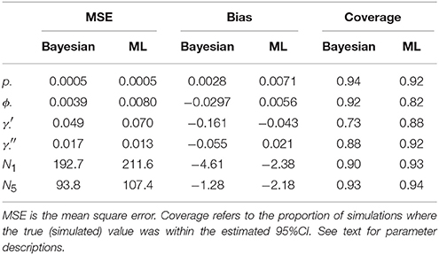
Table 1. Estimation properties of Bayesian and ML-based models over 100 simulations.

FIGURE 1

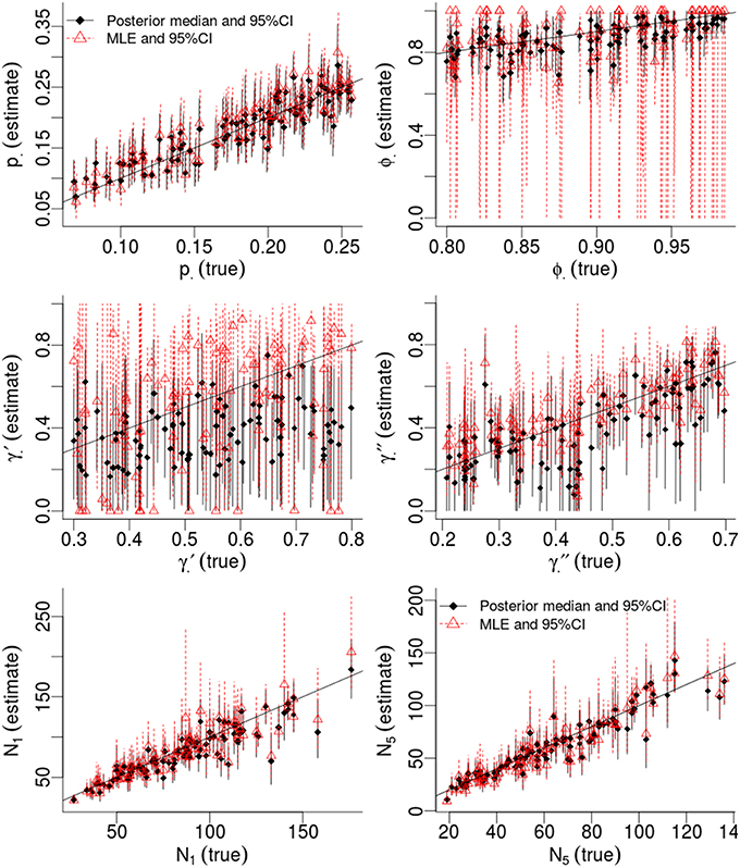
Figure 1. Results of a simulation-based study of Pollock's Closed Robust Design. Comparison of Maximum Likelihood Estimates and 95% Confidence Intervals (red; run in MARK) vs. Bayesian point estimates and 95% Credibility Intervals (black; run in JAGS). Notice different ranges for the x and y-axes.

Much of the inaccuracies in MARK estimates were a result of such boundary values. For example, 32% of ${\widehat{\varphi }}_{\mathrm{\text{MLE}}}$ became fixed at 1 and 15% of ${\widehat{\gamma }}_{\mathrm{\text{MLE}}}^{\prime }$ became fixed at 0. The former was much more likely to happen for high survival probabilities (e.g., ϕ_true > 0.95), while the latter did not seem to have a strong pattern in relation to other model specifications, but did seem slightly more common when values of γ′′ < 0.5. While such boundary values may indeed be the value which maximizes the data's likelihood, boundary estimates are problematic because their confidence intervals span the entire probability space, prohibiting meaningful conclusions and prohibiting the use of model-averaging techniques. Singularities never occurred in Bayesian models using Beta(1,1) priors. Instead, for those simulations which had boundary-value MLEs, the posterior densities merely took on more characteristics of their prior, and were nevertheless unimodal with finite 95%CI values.

Certain parameters showed moderate to high correlations in the variance-covariance matrices (Table 2). γ′ and ϕ were most strongly correlated, with mean coefficients 0.47 over all simulations, for both ML and Bayesian estimates, and reaching 0.95 in some ML estimates. p and γ′′ were also highly correlated with mean coefficients >0.4 in both ML and Bayesian techniques. However, despite the similarity in mean correlations, the range and distribution of correlations were generally very different between MLE and Bayesian models (Figure 2). For example, the correlation between the pair (γ′, ϕ) were somewhat uniform between 0 and 0.95 for Bayesian estimates, whereas the ML estimates clustered at two extremes: either 0 or around 0.9–0.95. The correlations for the pairs (γ′′, ϕ) and (γ′, γ′′) shared a similar pattern, whereby ML correlations were more extreme and clustered.

TABLE 2

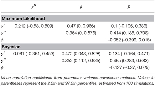
Table 2. Correlation in parameter estimates, summarized over 100 simulations.

FIGURE 2

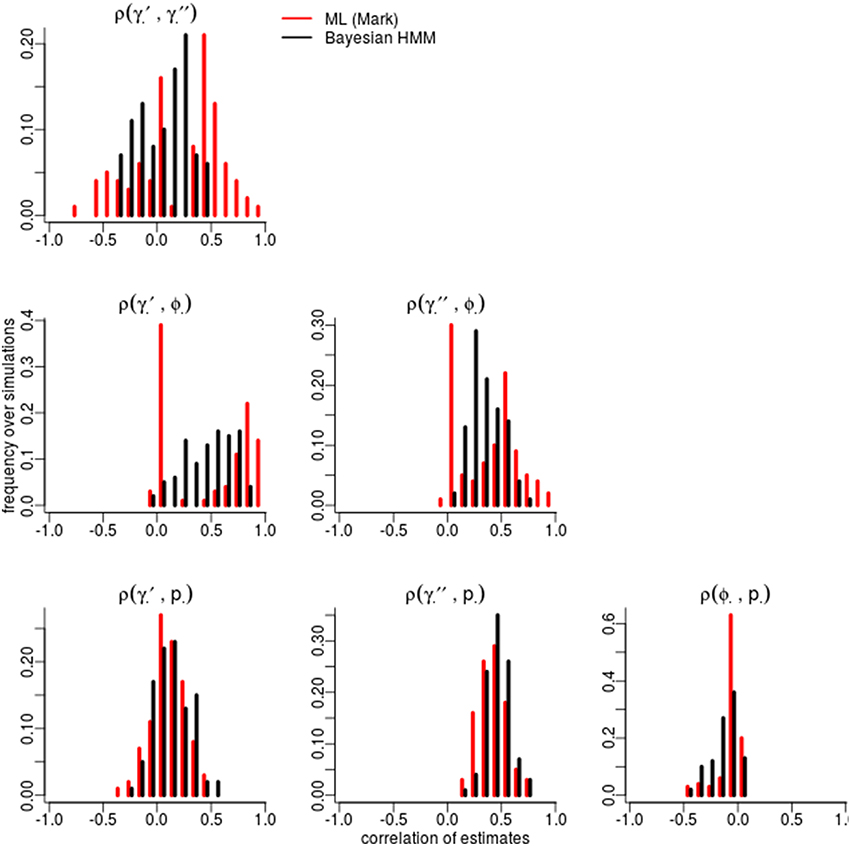
Figure 2. Correlation among parameters estimations over 100 simulations. The histograms compare the spread of correlations of parameter estimates by Maximum Likelihood (red; run in MARK) vs. the Bayesian non-hierarchical models (black; run in JAGS).

The sign and strength of parameter correlations also seemed to depend on the values of other parameters. These three-way relationships are too numerous to fully describe. However, it seemed that many correlations depended on values of p and γ′′. For example, with an effective detection probability of 0.69, the correlation between the pairs (ϕ, p) was between [−0.1, 0] for both ML and Bayesian methods, but strengthened to ≈ − 0.3 as the effective detection probability dropped to 0.22. Similarly, an effective detection probability of 0.69 yielded a correlation between (γ′′, p) of ≈0.4, which strengthened to ≈0.6 as the effective detection probability dropped to 0.22. Surprisingly, an opposite trend was seen between (ϕ, γ′) in relation to detection probability, such that increasing detection probabilities increased the strength of correlation between (ϕ, γ′). The other temporary migration parameter γ′′ also affected parameters' correlations; for example, the correlation between (γ′, γ′′) went from being negatively correlated (≈ − 0.2) to positively correlated (≈0.2) as γ′′ increased from 0.2 to 0.7. Likewise, the correlation between (γ′, p) had mostly zero correlation and became positively correlated (≈0.25) as γ′′ increased. Such three-way relationships were smoother and more gradual among the Bayesian estimates, whereas the ML values were much more extreme and clustered at high values, especially for ϕ, γ′, and γ′′.

3.2. Shark Bay Dolphins 1: Non-Hierarchical Bayesian PCRD

We analyzed the western gulf Shark Bay photo-identification data and found that all point estimates and intervals of all parameters and abundance estimates were nearly identical between ML estimation and four different Bayesian models. Figure 3 compares the state variables (ϕ, γ′, γ′′) and derived estimates of the population abundance, and the 28 detection probabilities.

FIGURE 3

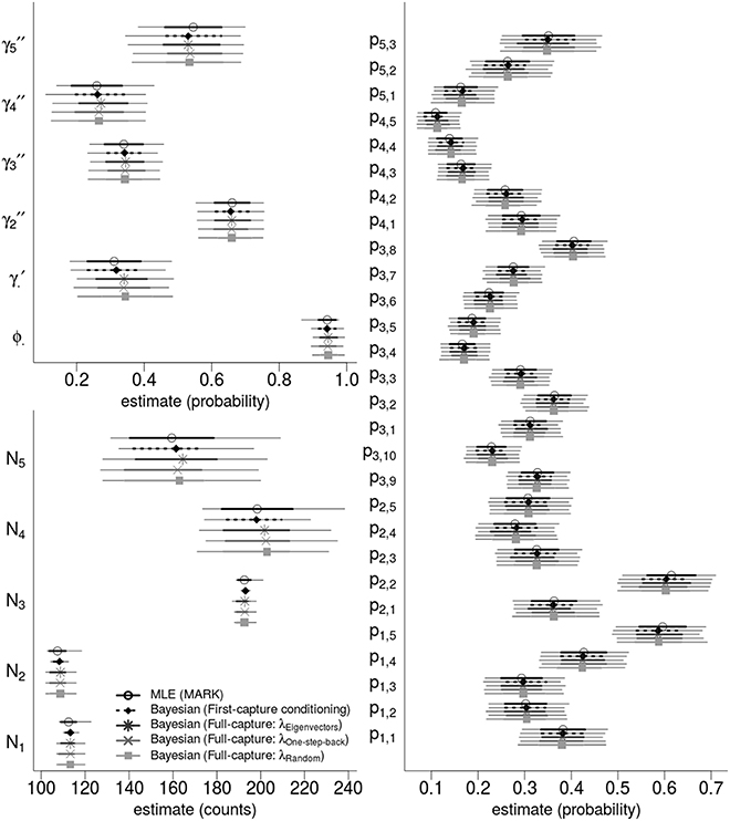
Figure 3. Bayesian and ML-based estimates: comparing state variables, population abundances, and detection probabilities for the western gulf Shark Bay bottlenose dolphins Tursiops aduncus. Comparison is among Maximum Likelihood estimation, and four different Bayesian Hidden Markov Models that use slightly different specifications for the recruitment process. Points are maximum likelihood and posterior mean estimators; thick intervals are 68.2% Confidence/Credibility Intervals (≈± 1 S.E.); thin intervals are 95%CIs. ϕ_· is the annual survival probability; ${\gamma }_{·}^{\prime }$ is the probability of remaining as a temporary migrant; ${\gamma }_t^{\prime \prime }$ are the time-varying probabilities of becoming a migrant; p_{t, s} are per-secondary period detection probabilities; N_t are the annual population of dolphins available for capture.

The four Bayesian full-capture models and one first-capture model all produced nearly identical results, irrespective of the specification of λ. However, the λ_{one-step-back} model took greater than 50 times longer to run than the λ_eigenvector and λ_random specifications for equal number of MCMC iterations.

The overall posterior predictive check p-values were: 0.300 (between-periods); 0.314 (within-periods); 0.244 (overall). While these exact values are not calibrated and cannot be easily interpreted, inspection of the individual elements of the m-array discrepancy statistics suggest that there may be issues with heterogeneous migration parameters (Table 3). In particular, recapture's in periods four and five had greater discrepancy for cohorts from the 2nd period as compared to cohorts from the 1st, 3rd, and 4th periods, suggesting there may be sub-populations with different migration dynamics. Inspection of the within-period discrepancies suggested that there was no issue with the assumption of population closure, given that all p_within values were ≈0.5.

TABLE 3

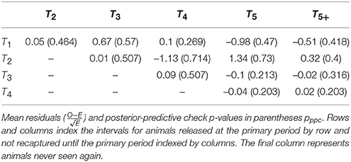
Table 3. Bayesian posterior predictive p-values for observed vs. expected elements of the open population m-array.

3.3. Shark Bay Dolphins 2: Hierarchical Bayesian vs. Model-Averaging

The top six fixed-effect models by AICc are listed in Table 4, representing >99.9% of the cumulative weights. Figure 4 compares the AICc model-averaged results to the different Hierarchical Bayesian (HB) results. The different HB prior specifications had nearly no effect on point estimates and intervals; instead, we saw a larger effect due to including or excluding individual random-effects for detection probabilities. Therefore, the pertinent comparisons are between the homogeneous-p_i HB model vs. the heterogeneous-p_i HB models [which include four models called target, stronger, weaker (1) and weaker (2)] vs. the MARK model-averaged estimates. For example, the AICc model-average and homogeneous-p_i HB estimates had much more similar estimates as compared to the four heterogeneous-p_i HB models.

TABLE 4

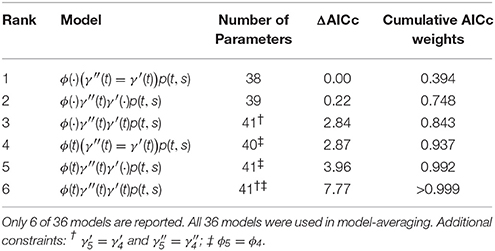
Table 4. Top six Pollock's Closed Robust Design fixed-effect models by AICc.

FIGURE 4

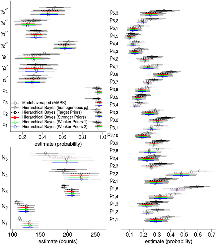
Figure 4. Hierarchical Bayes and model-averaging: comparison of estimates of state variables, population abundances, and detection probabilities for the western gulf Shark Bay bottlenose dolphins Tursiops aduncus. Comparison is among model-averaged fixed-effect models (by AICc weights), and four different Hierarchical Bayesian Hidden Markov Models with slightly different hyperpriors. The model labeled as “target” is our intended model for inference. Points are posterior mean estimators and model-averaged MLE; thick intervals are 68.2% Confidence/Credibility Intervals (≈± 1 S.E.); thin intervals are 95%CIs. ϕ_t are annual apparent survival probabilities; ${\gamma }_t^{\prime }$ are annual probabilities of remaining as a temporary migrant; ${\gamma }_t^{\prime \prime }$ annual probabilities of becoming a migrant; p_{t, s} are per-secondary period detection probabilities; N_t are the annual population of dolphins available for capture.

State parameters (γ, ϕ) were similar and had overlapping 68%CI across all models. However, the heterogeneous-p_i HB models had slightly lower γ estimates than the homogeneous-p_i and model-average estimates, i.e., a lower probability to leave the study area and remain outside. Model-averaged γ_t parameters seemed to have slightly more among-year variability than all HB models (both homo- and heterogeneous-p_i), consistent with the shrinkage-to-the-mean phenomenon imposed by the latter. Also, the heterogenous-p_i HB models had slightly higher survival ϕ estimates than the homogeneous-p_i HB and model-averaged estimates, with much tighter credibility intervals. All models showed little among-year variation in ϕ_t values.

Detection probability estimates were most sensitive to heterogeneous- vs. homogeneous-p_i specifications: consider that both model-averaged and homogeneous-p_i HB estimates consistently had p_{t, s} values which were 2 − 10 probability units larger than the heterogeneous-p_i HB models (albeit, with overlapping 68%CI's in most cases). This is an important result because there is nothing in the heterogeneous-p_i HB models that explicitly shrinks all the p_{t, s} parameters toward low values (see the Discussion for why we think heterogeneous-p_i would result in lower detection probabilities). We have no strong priors on the exact values or location of the p_{t, s} parameters; instead, our hyperpriors were focused on the between-period variability and within-period variability, and were deliberately weakly informative. We also observed less variability among detection probabilities within the same primary period in the HB models, compared to the model-averaged p_{t, s} values which were highly variable and nearly identical to the MLEs of fixed-effect “full-models” [i.e., estimates from a p(t, s) fixed-effect model]. Because we did not apply strong hyperpriors on the dispersion of detection probabilities, we suspect this shrinkage of detection probabilities to the mean-per-primary period is a consequence of assuming they share a common distribution, whereas ML and AIC methods assume they are completely independent.

There was a clear connection between different detection probabilities and population abundance. The effect of lower detection probabilities in the heterogeneous-p_i HB models as compared to the the model-averaged and homogeneous p_i model is apparent: the heterogeneous-p_i HB models estimated between 8.2 and 24.7% more dolphins than model-averaging or homogeneous-p_i model, with a median of 16.6% for N₂ (95%CI: 4.5–33.1%).

In order to assess the effect of our choice of hyperpriors on the posterior densities, Figure 5 compares the prior and posterior densities of the σ_θ parameters controlling the θ_t random-effects. In all cases, the ${\sigma }_{{\gamma }^{\prime }}$ and σ_ϕ posteriors were nearly identical to the target prior densities. Posterior densities were more similar to each other than their prior densities, suggesting that estimates were driven partially and significantly by the evidence in the data. The variation in γ′′ was much higher than our prior expectations. The largest change between prior and posterior densities occurred among the three densities controlling detection probability [σ_p(i), σ_p(t), σ_p(s)], and especially for σ_p(i), the dispersion among individual-level detection probabilities. For instance, the posterior expectation of σ_p(i) occurred in the 97.0th and 89.1th percentiles of the “target” and “weaker priors (2)” prior densities respectively. In other words, the data pushed the posterior mass away from the priors' expectation. Importantly, the posterior density of σ_p(i) was nearly identical among models, regardless of the different priors, suggesting that our estimate of σ_p(i) was mostly driven by the data. This gives very strong support for including individual-level random-effects.

FIGURE 5

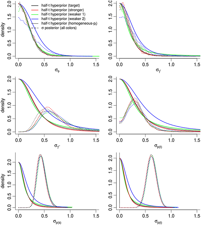
Figure 5. Posterior densities and half Student-t prior densities for σ_θ parameters controlling the dispersion of time-varying random-effects in a logit-Normal hierarchy. Different boxes are different parameters. Different colored lines represent different prior specifications, such that the priors labeled target are for our intended model for inference, while other colors inspect the sensitivity of the posterior to different priors. Thick lines are the priors; dashed-lines are the resulting posteriors. See the Appendix for exact specification of priors. Heights of the lines are re-scaled to faciliate density comparisons.

4. Discussion

This study presents a Bayesian Hidden Markov Model (HMM) version of the PCRD CMR model. We studied several versions which are appropriate for different model objectives and assumptions, such as conditioning on first-capture vs. recruitment modeling, and a hierarchical random-effects version vs. a non-hierarchical version. We studied the performance of the Bayesian method as compared to Maximum Likelihood estimation and model-averaging by analyzing simulated data as well as a real bottlenose dolphin dataset. Our main contributions and findings are the following:

• full-capture, non-hierarchical Bayesian PCRD models had slightly better estimation performance than equivalent fixed-effects ML estimation, mainly due to the latter's susceptibility to singularities (although there was no clear champion);

• we explored the partial non-identifiability and high correlation among parameter estimates, especially between γ′ and ϕ;

• using real data from a moderately-sized bottlenose dolphin population, we showed that inferences based on a fixed-effects ML model and a Bayesian (non-hierarchical) model were almost identical;

• we showed that various Bayesian methods to model recruitment and full-capture histories yielded nearly identical conclusions, both compared among each other and compared to a model that conditioned on first-capture; we motivate the use of full-capture Bayesian models to facilitate important extensions, such as individual-level random-effects;

• we developed a Hierarchical Bayesian PCRD which can lead to similar estimates as AICc model-averaging and serve as a type of multi-model inference;

• we showed how heterogeneity in detection probabilities can lead to a 8–24% increase in abundance estimates, as compared to ML and Bayesian models that assume homogeneous detection probabilities;

• we proposed two posterior predictive checks to help diagnose poor model fitting, in lieu of a formal goodness-of-fit procedure in popular CMR software.

4.1. Bayesian PCRD vs. MLE

A recurring result was the similarity and near equivalence of estimates between the Bayesian and ML-based methods, especially for simple “fixed-effect” models, but also among different Bayesian specifications, such as conditioning on first-capture and modeling the full-capture histories. This was supported by simulations and by analyzing a moderately-sized photo-ID dataset. In simulations, there was no unambiguous winner in terms of estimation performance, and both MLE and Bayesian estimates suffered from non-identifiability issues between temporary migration γ′ and survival ϕ. The frequency and similarity of correlations among parameter estimates in both ML-based and Bayesian PCRD points to a fundamental limitation of the model to resolve estimates in survival, and the issue warrants further study. While overall correlations were similar between Bayesian and ML-based estimates, one disadvantage of ML-based estimates was that their correlations were clustered at extreme values, such as either 0 or 1, which makes it difficult to diagnose such correlations post-hoc: the extreme values give the impression that either everything seems acceptable or is terrible. Researchers should attempt to deal with such problems at the study-design stage, such as increasing detection probability, increasing the number of primary periods or integrating auxiliary data into the analysis, especially observations of animals being alive or outside the study area when they may otherwise be classed as being in an unobservable state. For example, Bird et al. (2014) augmented CMR data with observations based on a telemetry study which included precise observations about when animals left the CMR study area.

A significant disadvantage of using ML estimation in Program MARK is its tendency for parameters to get stuck at boundary values, especially $\widehat{\varphi }=1$ and ${\widehat{\gamma }}^{\prime }=0$, such that CIs are undefined. This happened in 35% of simulations for at least one parameter, and, in our experience, is quite common for real data (but not in the case of the western gulf Shark Bay dolphins). Notably, in those cases where the MLE's get stuck at boundary values, the posterior distributions always had significant density away from the boundaries. These issues seem to happen more at low detection probabilities, high survival, and longer durations as a temporary migrant. Similar issues were noticed by Bailey et al. (2010) in multistate models with an unobservable state. We suggest that researchers who study animals that are long-lived and difficult to detect, such as marine mammals, should use Bayesian models with mildly informative priors, such as Beta(1,1), to avoid such singularities. It remains unclear whether reference priors and “objective Bayesian” analyses will likewise exhibit such beneficial behavior. However, there is evidence from the machine-learning and classification disciplines, that mild priors are necessary in situations of low sample sizes and multinomial models, in order to achieve sensible and stable estimates: a phenomenon called “Bayesian smoothing” (Murphy, 2012), whereby MLE's at unrealistic boundary values (0, 1) are pushed slightly toward their prior expectations, in lieu of strong evidence. In the case of CMR, low detection and high γ values relative to the number of primary periods can make it highly unlikely that one can observe enough “re-entries” to reliably estimate survival and migration processes.

4.2. Recruitment and the PCRD

Regarding our analysis of the bottlenose dolphin dataset, we interpret the near equivalence of Bayesian and ML estimates as a validation of the Bayesian HMM formulation and an opportunity for further development. While it is generally true that Bayesian posterior point-estimates should tend to the MLE values as the sample size and evidence increases, the equivalence among posterior expectations and ML estimates is not guaranteed in complex hierarchical models that integrate over many parameters (Hobbs and Hilborn, 2006). What is more interesting is the equivalence among the different full-capture and first-capture models: not only does this open the possibility of PCRD inference on recruitment processes (such as number of births or the population rate-of-increase), but it also facilitates more complex random-effects models, such as modeling individual heterogeneity. We were particularly interested in comparing slightly different specifications for the “recruitment ratio” (the proportion of new recruits that go to either latent state), which requires external data for reliable estimation (Wen et al., 2011), or a sensible nuisance process that can, at best, not bias other parameters. For bottlenose dolphins, we motivate the use of a computationally simple “eigenvector decomposition” which extrapolates a steady-state, unconditional probability of being inside or outside of the study area based on the marked population's migration parameters. Such direct calculation of the recruitment ratio from the marked population may only be sensible in a limited number of scenarios, such as when the recruits are not true ecological recruits, but are newly-marked conspecifics. In other words, such “apparent-recruits” share the same overall temporary migration patterns as their marked conspecifics. For other taxa who are highly migratory or whose apparent-recruits are true biological recruits, it would be inappropriate to use information from the marked population's migration parameters to inform the recruitment ratio. In such situations, a solution would be to include time-varying random variables for the recruitment ratio. Such a nuisance process would likely be driven entirely by the prior. Fortunately, Bayesian models and MCMC techniques allow us to integrate over such nuisance processes, which somewhat absolves us from worrying about the nuisance parameters' exact values. Therefore, the fact that such processes are not suitable for inference does not worry us, and we saw that the exact process did not bias or inflate the uncertainty of the other parameters. In our case, marginal point estimates and intervals among competing recruitment ratio specifications were nearly identical.

4.3. Hierarchical Bayesian PCRD

The similarity between fixed-effects Bayesian and ML estimates may not interest many modern CMR practitioners, but the results are important to lay the groundwork for more elaborate methods and other inference paradigms. For example, ecologists are increasingly preoccupied with “model uncertainty” and the sensitivity of their conclusions to arbitrary choices about parameter specifications, e.g. time-constant θ(·) vs. time-varying θ(t). To this end, we propose a Hierarchical Bayesian (HB) model as an alternative to the model-averaging methods popular in contemporary CMR practices. We suggest the HB method, not because of theoretical connections between the AIC model-averaging and Hierarchical Bayes, but instead appeal to the similarity in outcome between model-averaging and our shrinkage-inducing hyperpriors: both methods intend to smooth estimates between two extremes of θ(·) vs. θ(t). Others have pointed out this similarity (Gelman et al., 2004; Clark et al., 2005; Schofield et al., 2009), and Hooten and Hobbs (2015) describe how many multi-model inference techniques can be re-expressed as Bayesian models with particular priors.

We observed some slight differences between the HB models and the model-averaged estimates. For example, the model-average confidence intervals of survival estimates were nearly double those of HB, and HB had slightly lower γ_t estimates (which may be due to a bias in Bayesian ${\gamma }_t^{\prime }$ posteriors, as suggested in our simulations). Most importantly, the HB detection probabilities were shrunk toward the means of each primary period, whereas the model-averaged estimates were nearly identical to their fixed-effect values $\widehat{p}{(t,s)}_{\mathrm{\text{MLE}}}$. This latter point is perhaps one of the most crucial findings in this study, because population abundance estimates are very sensitive to the detection probabilities, and we must exercise some subjective judgment as to which model is most appropriate. For example, if we think that detections within a primary period are related to each other (e.g., by being co-correlated with other annually-varying influences such as climate, field crew, survey technology, etc.), then HB is most appropriate, and the independence assumed by ML estimation uses too many parameters. Under sparse data, over-parameterized PCRD models can result in MLEs occuring at unrealistic boundary values (e.g., ${\widehat{p}}_{t,s}=1$), with serious consequences for abundance estimates. In other words, the act of assuming a common distribution among detection probabilities, as compared to strict independence, can influence estimates in Hierarchical Bayesian models.

The ability of the Hierarchical Bayes to shrink time-varying parameters away from MLEs toward something less dispersed depends on the choice of the family of hyperprior distributions. We chose a logit-Normal prior distribution for time-varying state parameters and a scaled half Student-t hyperprior on the logit-Normals' dispersion parameters. This follows the work of Gelman (2006) who popularized the scaled half Student-t distribution for the dispersion parameters in Hierarchical Bayesian models (but not necessarily for CMR). Gelman argued for its use when shrinkage to zero is desirable and when there are < 5 grouping classes (consider that we have just three estimable parameters of ${\gamma }_t^{\prime }$ to define a distribution). Other common distributions on variance parameters, such as the Uniform or the Inverse-Gamma, are known to inflate variance when there are a small number of grouping classes. Currently, there is little literature on the use of different hyperpriors on random-effects in Hierarchical Bayes CMR models, and we look forward to more research in this area, and especially about explicit connections with other multi-model inference paradigms.

Readers from a Frequentist or Objective Bayesian background may be uncomfortable with what may be perceived as a casual use of both strongly informative and uninformative hyperpriors (Berger, 2006). It is a valid criticism which concerns all practitioners of subjective Bayesian analysis. But, for a practical mark-recapture problem, there are few alternatives which are objective, especially not ML-based nor model-averaging approaches. We defend our approach based on the following arguments. First, our sensitivity analyses suggest that slight variants of the hyperpriors did not change point-estimates and intervals of the realized state parameters. Secondly, nearly all Mark-Recapture analyses use model-averaging or model-selection (Johnson and Omland, 2004), and such multimodel techniques generally have a Bayesian interpretation; for example, the best model by AIC can actually be derived from a Bayesian model under a particular prior (Hooten and Hobbs, 2015). All model selection and model-averaging techniques depend on subjective decisions, ostensibly as the choice of how to score and rank models (e.g., AIC, BIC, QAIC, BMA), but are implicitly about one's preference for either maximizing predictive performance vs. in-sample fit, and how to penalize the effective number of parameters (Burnham, 2004; Hooten and Hobbs, 2015). The use of the QAIC is even less objective (White, 2002). Third, many subjective decisions are necessary to build a set of viable PCRD models, such as constraining parameters to avoid singularities, or by dropping singular models altogether. At worst, the totality of such arbitrary decisions can obfuscate the inference process. For example, in order for us to get finite intervals for model-averaged ϕ_t and ${\gamma }_t^{\prime }$ and ${\gamma }_t^{\prime \prime }$, we had to apply more constraints than what is prescribed in the literature. A real concern for science is the temptation of picking one's constraints or selection criteria to agree with one's hypothesis. Alternatively, the subjective Hierarchical Bayesian approach forces us to explicitly declare our beliefs a priori. Lastly, the hyperpriors we used were partially-motivated by the limitations of the PCRD model to estimate certain parameters, such as ${\gamma }_t^{\prime }$, especially under low samples sizes. To this point, it is well-known in applied fields like machine-learning that Bayesian priors are preferable to stabilize and smooth unstable and unreliable ML estimates in multinomial models under low sample sizes, a.k.a “Bayesian smoothing” (Murphy, 2012).

We juxtapose AIC-based model-averaging and HB in order to highlight how HB offers a compelling alternative to the fixed-effects model-selection problem: principly, through the use of a hyperprior to govern the shrinkage between θ(t) and θ(·) extremes. But, despite the similarity in estimates, the two paradigms are otherwise very different: only HB offers an intuitive, fully probabilistic model with posterior inference. CMR practitioners will be particularly interested in the easy ways to extend the HB model, such as incorporating individual random-effects, and other similar problems where the AIC is not defined.

4.4. Individual Heterogeneity

A much more significant impact on model estimates was the inclusion or exclusion of individual-level detection probabilities, rather than the exact values of our hyperpriors. Individual detection heterogeneity is a well-known phenomenon and perennial preoccupation of CMR practitioners (Carothers, 1973; Burnham and Overton, 1978; Clark et al., 2005). Unlike ML-based methods, heterogeneous detectability is a relatively simple extension in Hierarchical Bayesian models. Importantly, individual heterogeneity results in much lower mean detection probability estimates as compared to models which assume homogeneous detection probabilities, in both Bayesian or non-Bayesian models. Because population abundance estimates are sensitive to detection probabilities, this led us to conclude that there are actually 8–24% more marked individuals in the western gulf Shark Bay than previously estimated. We remind readers that the lowering of detection probabilities from heterogeneous detectability was not a consequence of a prior which intentionally shrunk the mean p_{t, s} values to zero (we had no such prior). Rather, we suggest that it was due to the full-capture history and random-effects framework and their ability to deflate the influence of outlier individuals. In other words, a CMR dataset inevitably has an over-representation of those individuals who are more detectable than others, and has an under-representation of those individuals who are less-detectable on average. Low-detectable individuals may be altogether absent from the dataset, given that they are more likely to be missed (Clark et al., 2005). This is a type of censoring, and Bayesian models are a well-known method to impute censored values and try to recover the true uncensored distribution. Ignoring such missing individuals will produce a “bottom-censored distribution” whose mean detection probability will be artifically higher than the true uncensored distribution; therefore, population abundance estimates will inevitably be lower in CMR datasets which fail to account for such “missingness.”

4.5. Future Work

Our proposed PCRD models are important to lay the foundations for several extensions. We anticipate extensions for a variety of challenges, such as increasing biological realism through mixture modeling, or integrated modeling of different datasets. Mixture modeling is particularly important because heterogeneity, in the form of mixtures of multiple unknowable subpopulations, is probably the rule in nature, rather than the exception. The latter point, about integrated modeling, will also be very important in the future, because a major result of our study was the frequency of very high correlations among parameter estimates. In both ML-based and Bayesian PCRD models, such correlations impose limits on the reliability of estimates, especially survival. Fortunately, the Bayesian framework and the flexible BUGS syntax opens the possibility to easily integrate other datasets, and one priority should be to remove some of the uncertainty of the unseen state. For example, the use of other opportunistic sightings or telemetry data outside the study area (Bird et al., 2014), can partially clarify the unseen “offsite” state, and thereby help reduce the correlation in temporary emigration and survival.

Author Contributions

RR conceived the central idea of the manuscript, conducted the statistical analyses and was the primary author of the manuscript. KP helped with the study design, conceived several core themes of the manuscript, supervised the analyses and helped edit the manuscript. KN was responsible for data collection and processing, consultation of the analyses and helped edit the manuscript. SA and MK helped design the study, collected data, managed data collection for the project and helped edit the manuscript. LB assisted with the study design and general supervision.

Conflict of Interest Statement

Prof Lars Bejder is an Associate Editor in the Marine Megafauna Section of Frontiers in Marine Science. Prof Kenneth H. Pollock is a Review Editor in the Marine Megafauna Section of Frontiers in Marine Science. The other authors declare that the research was conducted in the absence of any commercial or financial relationships that could be construed as a potential conflict of interest.

The reviewer MAM and handling Editor declared their shared affiliation, and the handling Editor states that the process nevertheless met the standards of a fair and objective review.

Acknowledgments

We would like to thank Shark Bay Resources and the Useless Loop community for ongoing logistical support for field activites under the Shark Bay Dolphin Innovation Project. This project was financially supported with grants from the Sea World Research and Rescue Foundation Inc., the A. H. Schultz Foundation Switzerland, Claraz–Schenkung Switzerland, Julius Klaus Foundation Switzerland, the National Geographic Society and the Winifred Violet Scott Foundation Australia. This manuscript represents publication number 10 from Shark Bay's Dolphin Innovation Project.

Supplementary Material

The Supplementary Material for this article can be found online at: https://www.frontiersin.org/article/10.3389/fmars.2016.00025

Please see the online tutorial at https://github.com/faraway1nspace/PCRD_JAGS_demo, including access to the bottlenose dolphin Photo-ID data used in this study, as well as JAGS code for running select models.

References

Bailey, L. L., Converse, S. J., and Kendall, W. L. (2010). Bias, precision, and parameter redundancy in complex multistate models with unobservable states. Ecology 91, 1598–1604. doi: 10.1890/09-1633.1

PubMed Abstract | CrossRef Full Text | Google Scholar

Berger, J. (2006). The case for objective Bayesian analysis. Bayesian Anal. 1, 385–402. doi: 10.1214/06-BA115

CrossRef Full Text | Google Scholar

Bird, T., Lyon, J., Nicol, S., McCarthy, M., and Barker, R. (2014). Estimating population size in the presence of temporary migration using a joint analysis of telemetry and capture-recapture data. Methods Ecol. Evol. 5, 615–625. doi: 10.1111/2041-210X.12202

CrossRef Full Text | Google Scholar

Brooks, S., and Gelman, A. (1998). General methods for monitoring convergence of iterative simulations. J. Comput. Graph. Stat. 7, 434–455.

Google Scholar

Brown, A., Bejder, L., Pollock, K. H., and Allen, S. J. (2016). Site-specific assessments of the abundance of three inshore dolphin species informs regional conservation and management. Front. Mar. Sci. 3:4. doi: 10.3389/fmars.2016.00004

CrossRef Full Text | Google Scholar

Brownie, C., Hines, J. E., Nichols, J. D., Pollock, K. H., and Hestbeck, J. (1993). Capture-recapture studies for multiple strata including non-Markovian transitions. Biometrics 49, 1173–1187. doi: 10.2307/2532259

CrossRef Full Text | Google Scholar

Burnham, K. P. (2004). Multimodel inference: understanding AIC and BIC in model selection. Sociol. Methods Res. 33, 261–304. doi: 10.1177/0049124104268644

CrossRef Full Text

Burnham, K. P., and Overton, W. S. (1978). Estimation of the size of a closed population when capture probabilities vary among animals. Biometrika 65, 625–633. doi: 10.1093/biomet/65.3.625

CrossRef Full Text | Google Scholar

Carothers, A. (1973). The effects of unequal catchability on Jolly-Seber estimates. Biometrics 29, 79–100. doi: 10.2307/2529678

CrossRef Full Text | Google Scholar

Clark, J. S., Ferraz, G., Oguge, N., Hays, H., and DiCostanzo, J. (2005). Hierarchical Bayes for structured, variable populations: from recapture data to life-history prediction. Ecology 86, 2232–2244. doi: 10.1890/04-1348

CrossRef Full Text | Google Scholar

Darroch, J. N. (1958). The multiple-recapture census: I. Estimation of a closed population. Biometrika 45, 343–359. doi: 10.2307/2333183

CrossRef Full Text | Google Scholar

Dupuis, J. A. (1995). Bayesian estimation of movement and survival probabilities from capture-recapture data. Biometrika 82, 761–772.

Google Scholar

Gelman, A. (2006). Prior distributions for variance parameters in hierarchical models. Bayesian Anal. 1, 515–533. doi: 10.1214/06-BA117A

CrossRef Full Text | Google Scholar

Gelman, A. (2013). Two simple examples for understanding posterior p-values whose distributions are far from unform. Electron. J. Stat. 7, 2595–2602. doi: 10.1214/13-EJS854

CrossRef Full Text | Google Scholar

Gelman, A., Carlin, J. B., Stern, H. S., and Rubin, D. B. (2004). Bayesian Data Analysis, 2nd Edn. Boca Raton, FL: Chapman & Hall/CRC.

Gelman, A., Meng, X., and Stern, H. (1996). Posterior predictive assessment of model fitness via realized discrepancies. Stat. Sin. 6, 733–759.

Google Scholar

Hobbs, N. T., and Hilborn, R. (2006). Alternatives to statistical hypothesis testing in ecology: a guide to self teaching. Ecol. Appl. 16, 5–19. doi: 10.1890/04-0645

PubMed Abstract | CrossRef Full Text | Google Scholar

Hooten, M., and Hobbs, N. T. (2015). A guide to Bayesian model selection for ecologists. Ecol. Monogr. 85, 3–28. doi: 10.1890/14-0661.1

CrossRef Full Text | Google Scholar

Johnson, J. B., and Omland, K. S. (2004). Model selection in ecology and evolution. Trends Ecol. Evol. 19, 101–108. doi: 10.1016/j.tree.2003.10.013

PubMed Abstract | CrossRef Full Text | Google Scholar

Kendall, W. L., and Nichols, J. D. (1995). On the use of secondary capture-recapture samples to estimate temporary emigration and breeding proportions. J. Appl. Stat. 22, 751–762. doi: 10.1080/02664769524595

CrossRef Full Text | Google Scholar

Kendall, W. L., Nichols, J. D., and Hines, J. E. (1997). Estimating temporary emigration using capture-recapture data with pollock's robust design. Ecology 78, 563–578.

Google Scholar

Kendall, W. L., and Pollock, K. H. (1992). “The robust design in capture-recapture studies: a review and evaluation by Monte Carlo simulation,” in Wildlife 2001: Populations, eds D. R. McCullough and R. H. Barrett (Springer), 31–43. Available online at: http://www.springer.com/us/book/9781851668762?wt_mc=ThirdParty.SpringerLink.3.EPR653.About_eBook

Kendall, W. L., Pollock, K. H., and Brownie, C. (1995). A likelihood-based approach to capture-recapture estimation of demographic parameters under the robust design. Biometrics 51, 293–308. doi: 10.2307/2533335

PubMed Abstract | CrossRef Full Text

Kèry, M., and Schaub, M. (2011). Bayesian Population Analysis Using WinBUGS: A Hierarchical Perspective. Oxford, UK: Academic Press.

Laake, J. L. (2013). “RMark: an R interface for analysis of capture-recapture data with MARK,” in AFSC Processed Report 2013-01 (Seattle, WA: Alaska Fisheries Science Center; NOAA's National Marine Fisheries Service).

Lebreton, J., Nichols, J. D., Barker, R. J., Pradel, R., and Spendelow, J. A. (2009). “Modeling individual animal histories with multistate capture recapture models,” in Advances in Ecological Research, Vol. 41, ed H. Caswell (Academic Press), 87–173.

Lebreton, J.-D., Almeras, T., and Pradel, R. (1999). Competing events, mixtures of information and multistratum recapture models. Bird Study 46, S39–S46. doi: 10.1080/00063659909477230

CrossRef Full Text | Google Scholar

Murphy, K. P. (2012). Machine Learning: A Probabilistic Perspective. Cambridge, MA: MIT press.

Google Scholar

Nicholson, K., Bejder, L., Allen, S. J., Krützen, M., and Pollock, K. H. (2012). Abundance, survival and temporary emigration of bottlenose dolphins (Tursiops sp.) off Useless Loop in the western gulf of Shark Bay, Western Australia. Mar. Freshw. Res. 63, 1059–1068. doi: 10.1071/MF12210

CrossRef Full Text | Google Scholar

Plummer, M. (2014). rjags: Bayesian Graphical Models Using MCMC. R package version 3-13.

Pollock, K. H. (1982). A capture-recapture design robust to unequal probability of capture. J. Wildl. Manage. 46, 752–757. doi: 10.2307/3808568

CrossRef Full Text | Google Scholar

Pollock, K. H., and Nichols, J. D. (1990). Statistical inference for capture-recapture experiments. Wildl. Monogr. 107, 4.

Google Scholar

Pradel, R. (1996). Utilization of capture-mark-recapture for the study of recruitment and population growth rate. Biometrics 52, 703–709. doi: 10.2307/2532908

CrossRef Full Text | Google Scholar

R Core Team (2014). R: A Language and Environment for Statistical Computing. Vienna.

Royle, J. A., and Dorazio, R. M. (2012). Parameter-expanded data augmentation for Bayesian analysis of capture-recapture models. J. Ornithol. 152, 521–537. doi: 10.1007/s10336-010-0619-4

CrossRef Full Text | Google Scholar

Royle, J. A., and Kèry, M. (2007). A Bayesian state-space formulation of dynamic occupancy models. Ecology 88, 1813–1823. doi: 10.1890/06-0669.1

PubMed Abstract | CrossRef Full Text | Google Scholar

Schofield, M. R., and Barker, R. J. (2011). Full open population capture-recapture models with individual covariates. J. Agric. Biol. Environ. Stat. 16, 253–268. doi: 10.1007/s13253-010-0052-4

CrossRef Full Text | Google Scholar

Schofield, M. R., Barker, R. J., and Mackenzie, D. I. (2009). Flexible hierarchical mark-recapture modeling for open populations using WinBUGS. Environ. Ecol. Stat. 16, 369–387. doi: 10.1007/s10651-007-0069-1

CrossRef Full Text | Google Scholar

Smith, H. C., Pollock, K., Waples, K., Bradley, S., and Bejder, L. (2013). Use of the robust design to estimate seasonal abundance and demographic parameters of a coastal bottlenose dolphin (Tursiops aduncus) population. PLoS ONE 8:e76574. doi: 10.1371/journal.pone.0076574

PubMed Abstract | CrossRef Full Text | Google Scholar

Tanner, M., and Wong, W. (1987). The calculation of posterior distributions by data augmentation. J. Am. Stat. Assoc. 82, 528–540. doi: 10.1080/01621459.1987.10478458

CrossRef Full Text | Google Scholar

Wen, Z., Pollock, K., Nichols, J., and Waser, P. (2011). Augmenting superpopulation capture-recapture models with population assignment data. Biometrics 67, 691–700. doi: 10.1111/j.1541-0420.2010.01522.x

PubMed Abstract | CrossRef Full Text | Google Scholar

White, G. C. (2002). Discussion comments on: the use of auxiliary variables in capture-recapture modelling. An overview. J. Appl. Stat. 29, 103–106. doi: 10.1080/02664760120108476

CrossRef Full Text | Google Scholar

White, G. C., and Burnham, K. P. (1999). Program MARK: survival estimation from populations of marked animals. Bird Study 46, S120–S139. doi: 10.1080/00063659909477239

CrossRef Full Text | Google Scholar