On the Decadal Trend of Global Mean Sea Level and Its Implication on Ocean Heat Content Change

Introduction

The decadal variability of the trend of the global mean sea level (GMSL) is of great importance to studying its long-term evolution as well as the associated change of the heat content of the ocean. Most climate time series such as the sea level record are characterized by a red noise process (e.g., Wunsch, 1999). The temporal correlation of the residuals from a linear trend fit has often been neglected in estimating the uncertainly of the fit, leading to underestimate of its errors. In this study the problem is treated as optimal estimation to minimize the residuals weighted by the autocovariance of the time series. The approach takes into account the variability of the time series over various time scales, and the subsequent effects on the estimate of a trend and its uncertainty.

Satellite radar altimetry has been applied to the measurement of the GMSL since the launch of the TOPEX/Poseidon Mission in 1992 (Nerem et al., 2010; Masters, 2012; Henry, 2014; Ablain et al., 2015; Dieng et al., 2015b). The systematic error in the altimetric sea level trend, a bias drift, has been estimated from comparison to tide gauge observations, which have long-term (multi-decade scales) errors from land motions (Mitchum, 2000; Watson, 2015), which include the errors in the terrestrial reference frame (Collilieux and Woppelmann, 2011; Haines et al., 2015). After the bias drift correction, the remaining errors are primarily caused by the uncertainty in the knowledge of the vertical land motions at the tide gauge locations. The time scale of the vertical land motions is tectonic and generally much longer than a decade. These errors essentially cause a bias in the estimate of a trend over decadal scales. Such bias would be canceled for evaluating the change of decadal trends, of which the errors are dominated by the uncertainty in the estimation error.

As the contribution to sea level change from the change in ocean mass can be estimated from space gravimetry missions like GRACE (Johnson and Chambers, 2013). The variation of the global mean steric sea level can be estimated from the combination of altimetry and GRACE observations (Willis et al., 2008; von Schuckmann, 2014; Dieng et al., 2015a). The results have been compared to the observations made by Argo in the upper ocean. Although the results have substantial uncertainty, it is interesting to examine the decadal trend error of the global mean steric sea level for making inference on the rate of the change of the ocean heat content. This is an important indicator for the heat balance of the globe as more than 90% of the heat accumulated on Earth over the past century has been stored in the ocean (Levitus, 2012).

Methodology

The problem of fitting to a time series by a polynomial can be readily formulated as an optimal estimation problem (e.g., Wunsch, 1996). For the sake of clarity, the methodology described in Wunsch (1996) is briefly summarized here. The linear trend, denoted by b, can be solved for in the following equation:

$\begin{array}{ll}a+bt+n\left(t\right)=y\left(t\right)& (1)\end{array}$

where a represents a constant, n(t) random noise, and y(t) the time series of observations at time t. Equation (1) can be written the following form:

$\begin{array}{ll}Da+n=y& (2)\end{array}$

Where

$\begin{array}{ll}D=\left\{\begin{array}{ll}\hfill & \begin{array}{ll}1\hfill & t_1\hfill \\ 1\hfill & t_2\hfill \end{array}\hfill \\ \hfill & .\hfill \\ \hfill & .\hfill \\ \hfill & \begin{array}{ll}1\hfill & t_m\hfill \end{array}\hfill \end{array}\right\},a=\left[\begin{array}{c}a\\ b\end{array}\right],y=\left[\begin{array}{c}y(t_1)\\ \begin{array}{ll}\hfill & y(t_2)\hfill \\ \hfill & .\hfill \\ \hfill & .\hfill \\ \hfill & y(t_m)\hfill \end{array}\end{array}\right],& (3)\end{array}$

and n(t) is the noise vector. Let the m × m autocovariance matrix of y be noted by R, then the optimal solution for a is expressed as follows (Wunsch, 1996, p. 121):

$\begin{array}{ll}\tilde{a}=\left[\begin{array}{c}\tilde{a}\\ \tilde{b}\end{array}\right]={\left[D^T{R}^{-1}D\right]}^{-1}{D}^T{R}^{-1}y& (4)\end{array}$

The variance of the uncertainty of the estimate ã about its mean is

$\begin{array}{ll}P=<{(\tilde{a}-a)}^2>={\left[D^T{R}^{-1}D\right]}^{-1}& (5)\end{array}$

The autocovariance matrix R is given below:

$\begin{array}{ll}\left[\begin{array}{ccccc}R(0)& R(\Delta t)& R(2\Delta t)& .& R((m-1)\Delta t)\\ R(\Delta t)& R(0)& R(\Delta t)& .& R((m-2)\Delta t)\\ .& .& .& .& .\\ R((m-1)\Delta t)& & .& .& R(0)\end{array}\right]& (6)\end{array}$

Where Δt is the interval of the time series y and the matrix elements are the autocovariance of y after a linear trend is removed. R thus represents the covariance of the error of estimating a linear fit to the time series y. The solution for ã from Equation (4) has minimum variance of uncertainty via a weighted least-squares approach. For the relatively short record of satellite altimetry measurement, the estimation error of R increases with time scales. The validity of the results on the decadal scales has been examined by comparison to the standard linear regressions analysis with the degrees of freedom determined by R.

Results

Sea Level

Displayed in Figure 1 is the GMSL time series obtained from satellite altimeter measurements by TOPEX/Poseidon and its successors Jason-1 and Jason-2 (Nerem et al., 2010). The data were processed by the Sea Level Research Group of the University of Colorado (CU) with the seasonal cycle removed. The estimates of the sea level trend are somewhat different among the results from various groups, owing to the differences in treating the time-variable biases in the radiometer corrections, the sea-state bias models, the inter- and intra-mission biases, and the differing orbits (Dieng et al., 2015b). However, the result of the CU has the least residual trend (−0.03 mm/yr) after subtracting ocean mass from GRACE and steric sea level from Argo. This near closure of the sea level budget indicates the consistency of the CU record with other types of observation to the extent of their uncertainties.

FIGURE 1

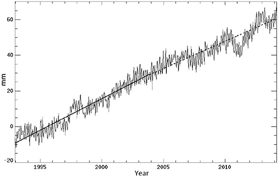
Figure 1. GMSL (in mm) time series in 10-day intervals from 1993–2013, obtained from the altimeter measurements from the TOPEX/Poseidon, Jason-1, and Jason-2 missions (Nerem et al., 2010). The heavy solid and dashed lines represent linear fits of the first and second half of the record, respectively. The standard deviation of the random errors is 4.1 mm.

In this study, it is assumed that the uncertainty in the sea level trend from the CU record consists in a systematic measurement error and the trend estimation error. With the seasonal cycle removed, the trend of sea level rise was estimated by the CU group to be 3.3 ± 0.4 mm/yr. The uncertainty was estimated from comparison to the observations from a global tide gauge network. As discussed in Mitchum (2000) and Watson (2015), the uncertainty is a systematic error dominated by that of the tide gauge observations caused by the land motions at the sites of the gauges. The errors in the terrestrial reference frame are imbedded in the land motion errors as well as manifested in orbit errors which have been estimated to be ~0.3 mm/yr (Beckley et al., 2007) for the period of 1993–2007. The trend estimation error was considered to be < 0.1 mm/yr and ignored in the total error estimate of Nerem et al. (2010). The underlying causes for the systematic error from the slowly evolving land motions and the terrestrial reference frame have time scales much longer than a decade after the seasonal cycle is removed from the record. The systematic error is thus negligible in the determination of a trend on decadal scales.

With the increasing length of the record, we are often faced with questions like “How has the rate of sea level rise changed over the recent past? Is the change significant from decade to decade?” To answer such questions with quantified degree of certainty requires a rigorous estimate of the uncertainty in the estimate of a trend. To address possible change of the trend on decadal scales and its statistical significance, also shown in Figure 1 are the linear fits to the first and the second half of the record computed using Equation (4), exhibiting slightly different rates: 3.54 ± 0.29 mm/yr for the first decade; 3.06 ± 0.31 mm/yr for the second decade. The purpose of this study is not about the reason for the apparent change of the trend, but the statistical uncertainty arising from the correlated signals. The error bars are estimated by taking the square root of the values obtained from Equation (5), with the auto-covariance of the sea level time series shown in Figure 2. The peak, ~17 mm², at zero lag corresponds to the variance of the random error after averaging the altimeter data over the 10–day repeat cycles. It corresponds to an error bar (standard deviation) of 4.1 mm for each 10-day data point in the time series.

FIGURE 2

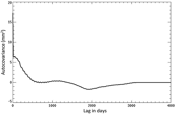
Figure 2. The auto covariance of the time series shown in Figure 1.

In practice, the autocovariance was obtained by applying the inverse Fourier Transform to the power spectrum of the GMSL time series after a linear trend is removed (Figure 3). The low-frequency plateau indicates the “red” nature of the time series dominated by the long time scales. There is a peak around 60 days associated with residual tidal and orbital errors. This peak is overwhelmed by the wide-band low-frequency signals that dominate the autocovariance. The correlation time scale of the time series, τ, can be estimated by Kendall and Stuart (1976)

$\begin{array}{ll}\tau =2{\displaystyle \sum _{i=0}^{m-1}\frac{R^2(i\Delta t)}{R^2(0)}\Delta t}& (7)\end{array}$

The evaluation of Equation (7) leads to τ = 480 days. The correlated error of this time scale is accounted for in the minimum variance solution from Equation (4). Without accounting for the correlated error and assuming that each data point is independent, the standard error of the trend estimate of a 10-year record would be about 0.07 mm/yr, a severe underestimate compared to ~0.3 mm/yr. Using Equation (4) the trend of the whole 22-year record is 3.28 ± 0.10 mm/yr. Note that the trend error without accounting for the correlated error would be 0.025 mm/yr.

FIGURE 3

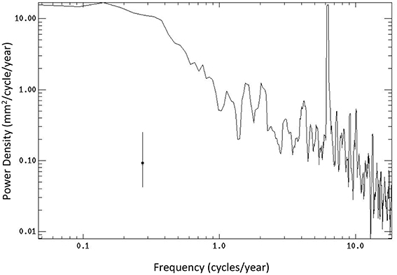
Figure 3. The frequency spectrum of the time series shown in Figure 1 with a linear trend removed. The error bar represents the 95% confidence interval.

To test the validity of the estimate of the correlation time scale from Equation (7), the time series shown in Figure 1 was smoothed over 480 days and resampled at the same interval. Then each of the resampled 16 data points should be independent. The linear trend was estimated with 16 degrees of freedom resulting in 3.20 ± 0.09 mm/yr. Note that the uncertainty is close to 0.10 mm/yr derived from the optimal estimation. This provides a consistency test of the accuracy of the autocovariance function and its role in Equations (4) and (7).

The fact that the two trend estimates are separate by more than one standard deviation suggests that the rate of sea level rise in the second decade is significantly less than in the first decade. Assuming the error statistics are Gaussian, the probability for the above statement being true is estimated 87% based on the trend values and respected standard deviations. The quantification of the uncertainty in the decadal change of the rate of sea level rise is important for determining the long-term evolution of the GMSL in terms of acceleration or deceleration.

Although there have been studies on the interannual variability of the GMSL in terms of the global hydrological cycle (e.g., Cazenave, 2014), there have been no explanations for the apparent deceleration on decadal scales until the study by Watson (2015). They used an improved tide gauge database for making altimeter bias drift correction. After the correction, the GMSL rose at a much slower rate over the first 6 years of the TOPEX/Poseidon record, which suffered from instrument degradation until the altimeter switched to a redundant side in 1999. As noted earlier, the present study does not address the physical mechanism of the variability of the decadal trend nor the altimeter bias drift correction, but only focus on the effects of correlated signals on the uncertainty in the decadal trend.

Ocean Heat Content

Another important piece of information from the decadal change of the rate of sea level rise is the change of the ocean heat content reflected by the steric component of sea level. As noted in the Introduction, steric sea level can be determined from the difference between altimeter-measured GMSL and GRACE-measured mass component. The GRACE data processed by the Center for Space Research of the University of Texas at Austin and analyzed by Llovel et al. (2014) were used for the present study. The data products from other groups have shown small differences (±0.08 mm/yr; Dieng et al., 2015b). The altimeter-determined GMSL (Figure 1) was smoothed over 60 days and subsampled at monthly intervals to match the GRACE data in the period of 2003–2013 as in Llovel et al. (2014). Shown in Figure 4 is the steric sea level computed by subtracting the mass component from the GMSL. The rate of the rise estimated from Equation (4) is 0.88 ± 0.12 mm/yr. Not included in the error estimate are the long-term systematic errors of both altimetry and GRACE. The long-term 0.4 mm/yr error in the altimetry measurement is discussed previously. The dominant systematic error in the GRACE measurement is caused by the uncertainty in the correction for the Glacial Isostatic Adjustment. It is also estimated to be 0.4 mm/yr (Chambers et al., 2010) with a time scale longer than decadal and can be ignored in decadal trend error.

FIGURE 4

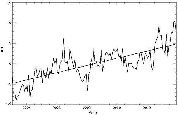
Figure 4. The steric sea level obtained from the altimeter and GRACE data. The straight line shows a linear fit of the curve.

Compared to the estimate of Llovel et al. (2014), 0.77 ± 0.28 mm/yr, the new estimate is a larger trend with less error. The differences are partly caused by the effect of the correlated signals accounted for in the present study. The larger uncertainty of Llovel et al. (2014) was probably caused by the fact that their uncertainty estimate was a combination of the formal fit error (without accounting for the correlated signals) and the random observational error as described in their paper. The present approach has taken into account both the observational error and correlated signals by the use of the autocovariance function. In any case, the two estimates are within the quoted statistical uncertainties of each.

Based on global ocean climatologic conditions, Wunsch and Heimbach (2014) estimated the equivalence between the rate of sea level rise and the rate of ocean warming: 1 mm/yr corresponds to 0.75 W/m². This implies that the 1-sigma uncertainly in the rate of ocean warming on decadal scales determined from that of the steric sea level, 0.12 mm/yr, is close to 0.1 W/m². This is consistent with the estimate of Wunsch and Heimbach (2014) from model-based ocean state estimation. Given the estimated global ocean warming rate of 0.5–1 W/m² (Hansen, 2005; Roemmich and, 2015), the 0.1 W/ m² error provides an order of magnitude guide for determining if there is significant change in the ocean warming rate on decadal scales. The result suggests that the temporally correlated signals in the altimeter and GRACE observations have an effect comparable to the uncertainty of the Argo observations in the determination of the decadal trend of the ocean heat content. The contribution of the deep ocean is much less than the uncertainty of the heat budget on decadal scales.

Systematic Errors

Llovel et al. (2014) used the Argo data from 2005 to 2013 to estimate the steric sea level from the temperature and salinity observations of the upper 2000 m of the ocean. They obtained a linear trend of 0.90 ± 0.15 mm/yr, which is the average of 5 data products from Argo. The steric sea level derived from the altimeter and GRACE data over the same period is 0.82 ± 0.17 mm/yr. The two estimates are not distinguishable to the extent of the estimated uncertainty, consistent with the findings of Llovel et al. (2014). Note that the steric sea level from the water below 2000 m is about 0.1 ± 0.1 mm/yr from direct observations (Purkey and Johnson, 2010), which is less than the uncertainties of both the Argo and satellite observations. The close agreement given above is a mutual validation of the Argo and satellite observations (Willis et al., 2010). Dieng et al. (2015b) presented the range of results from various Argo data products, showing small differences on the order of ± 0.08 mm/yr, which is smaller than the formal uncertainty of ± 0.15 mm/yr. However, we must keep this uncertainty in mind when interpreting the result of the present study, which is focused on the statistical uncertainty of the trend estimation.

The comparison of the steric sea level determined from Argo to the space observations from altimetry and GRACE provides an opportunity to assess the systematic errors of the space observations during the period when the three observations coexist. If we add the contribution from the deep ocean noted above, 0.1 ± 0.1 mm/yr, to the contribution from the upper ocean, 0.90 ± 0.15 mm/yr, we obtain 1.0 ± 0.18 mm/yr (the uncertainty is the root-sum-squares of the two) for the total steric sea level. Its difference from the space observation, 0.82 ± 0.17 mm/yr, yields 0.18 ± 0.25 mm/yr. Given the various assumptions noted earlier, this provides an estimate of the combined systematic errors of altimetry minus GRACE measurements during the period of coexistence of the three measurements, 2005–2013. The systematic errors of the measurement systems are likely to change with time, as indicated for example by the relatively large altimeter bias drift in the early part of the altimetry record of TOPEX/Poseidon (Watson, 2015)

Conclusions

The formal error in estimating a linear trend in the GMSL record is treated as a problem of optimal estimation. The temporally correlated variability of the record is accounted for by its autocovariance. For the 22-year record from the TOPEX/Poseidon, Jason-1, and Jason-2 missions, a linear trend of 3.28 ± 0.10 mm/yr is obtained. The overall error in estimating a bias drift from comparison to a network of globally distributed tide gauges is estimated to be 0.4 mm/yr (Mitchum, 2000). This error is primarily caused by the uncertainty in the vertical land motions at the tide gauge locations. The time scale of the variability of the uncertainty is associated with the long-term change of the solid earth and is much longer than a decade. On decadal time scales, the uncertainty in detecting a change of the trend of sea level has significant contribution from the formal error of the trend estimate, which is about 0.3 mm/yr for a 10-year record.

The mass component of the variation of the GMSL during 2003–2013 is determined from the gravity measurement from the GRACE mission. Subtraction of the mass component from the altimeter-determined sea level leads to an estimate of the global mean steric sea level, which exhibits a trend of 0.88 ± 0.12 mm/yr over the 10 year period. This corresponds to oceanic heat absorption at a rate of 0.66 ± 0.09 W/m². Although the absolute value is subject to an unknown bias on time scales longer than a decade, the error estimate applies to the uncertainty on a decadal scale. It is considered that the uncertainty in detecting a decadal change in the rate of oceanic heat uptake based on satellite altimetry and gravimetry measurement is on the order of 0.1 W/m². However, the contributions from the regions not covered by the satellite observations have been neglected (the ocean below 2000 m, the Arctic Ocean and other marginal seas).

The estimate of the steric sea level from altimetry and GRACE is subject to long-term systematic errors: approximately 0.4 mm/yr error in both the altimetry measurement and the GRACE measurement. The difference between of the steric sea level, estimated from Argo plus the estimated deep ocean contribution, and that from altimeter and GRACE, 0.18 ± 0.25 mm/yr, provides an estimate of the combined systematic errors of altimetry minus GRACE observations during 2005–2013. Longer records of altimetry, gravity, and Argo will shed light on the long-term stability of the systematic errors and the utility of spaceborne observations to determining the steric sea level and associated change in ocean heat content.

Author Contributions

The author confirms being the sole contributor of this work and approved it for publication.

Conflict of Interest Statement

The author declares that the research was conducted in the absence of any commercial or financial relationships that could be construed as a potential conflict of interest.

Acknowledgments

The data used in the study is available at (1) Altimeter data: The University of Colorado Sea Level Research Group, URL: http://sealevel.colorado.edu/; (2) GRACE data were processed by the Center for Space Research of the University of Texas at Austin (release-5) and available at: NASA Physical Oceanography Distributed Active-Archive Center, URL: ftp://podaac-ftp.jpl.nasa.gov/allData/grace/L2/CSR/RL05. The research presented in the paper was carried out at the Jet Propulsion Laboratory, California Institute of Technology, under contract with the National Aeronautic and Space Administration. Discussions with Carl Wunsch of Harvard University, as well as with Felix Landerer and Josh Willis of JPL are gratefully acknowledged.

References

Ablain, M., Cazenave, A., Larnicol, G., Balmaseda, M., Cipollini, P., Faugère, Y., et al. (2015). Improved sea level record over the satellite altimetry era (1993-2010) from the climate change initiative project. Ocean Sci. 11, 67–82. doi: 10.5194/os-11-67-2015

CrossRef Full Text | Google Scholar

Beckley, B. D., Lemoine, F. G., Luthcke, S. B., Ray, R. D., and Zelensky, N. P. (2007). A reassessment of global and regional mean sea level trends from TOPEX and Jason-1 altimetry based on revised reference frame and orbits. Geophys. Res. Lett. 34, L14608. doi: 10.1029/2007GL030002

CrossRef Full Text | Google Scholar

Cazenave, A. (2014). The rate of sea-level rise. Nat. Clim. Change 4, 358–361. doi: 10.1038/nclimate2159

CrossRef Full Text | Google Scholar

Chambers, D. P., Wahr, J., Tamisiea, M. E., and Nerem, R. S. (2010). Ocean mass from GRACE and glacial isostatic adjustment. J. Geophys. Res. 115, B11415. doi: 10.1029/2010JB007530

CrossRef Full Text | Google Scholar

Collilieux, X., and Woppelmann, G. (2011). Global sea-level rise and its relation to the terrestrial reference frame. Geod. J. 85, 9–22. doi: 10.1007/s00190-010-0412-4

CrossRef Full Text | Google Scholar

Dieng, H. B., Cazenave, A., von Schuckmann, K., Ablain, M., and Meyssignaac, B. (2015b). Sea level budget over 2005-2013: missing contributions and data errors. Ocean Sci. Discuss. 12, 701–734. doi: 10.5194/os-11-789-2015

CrossRef Full Text

Dieng, H. B., Palanisamy, H., Cazenave, A., Meyssignac, B., and von Schuckmann, K. (2015a). The sea level budget since 2003: inference on the deep ocean heat content. Surd. Geophys. 36, 209–229. doi: 10.1007/s10712-015-9314-6

CrossRef Full Text | Google Scholar

Haines, B. J., Bar-Sever, Y. E., Bertiger, W. I., Desai, S. D., Harvey, N., Sibois, A. E., et al. (2015). Realizing a terrestrial reference frame using the global positioning system. J. Geophys. Res. Solid Earth 120, 5911–5939. doi: 10.1002/2015JB012225

CrossRef Full Text | Google Scholar

Hansen, J. (2005). Earth's energy imbalance: confirmation and implications. Science 308, 1431–1435. doi: 10.1126/science.1110252

PubMed Abstract | CrossRef Full Text | Google Scholar

Henry, O. (2014). Effect of the processing methodology on satellite altimetry-based GMSL rise over the Jason-1 operating period. Geod. J. 88, 351–361. doi: 10.1007/s00190-013-0687-3

CrossRef Full Text | Google Scholar

Johnson, G. C., and Chambers, D. P. (2013). Ocean bottom pressure seasonal cycles and decadal trends from GRACE Release-05: Ocean circulation implications. J. Geophys. Res. Oceans 118, 4228–4240. doi: 10.1002/jgrc.20307

CrossRef Full Text | Google Scholar

Kendall, M., and Stuart, A. (1976). The Advanced Theory of Statistics, Vol. 3, 3rd Edn. London: Griffin.

Google Scholar

Levitus, S. (2012). World ocean heat content and thermosteric sea level change (0–2000 m), 1955–2010. Geophys. Res. Lett. 39, L10603. doi: 10.1029/2012GL051106

CrossRef Full Text | Google Scholar

Llovel, W., Willis, J. K., Lander, F. W., and Fukumori, I. (2014). Deep-ocean contribution to sea level and energy budget not detectable over the past decade. Nat. Clim. Change 4, 1031–1035. doi: 10.1038/nclimate2387

CrossRef Full Text | Google Scholar

Masters, D. (2012). Comparison of GMSL time series from TOPEX/Poseidon, Jason-1, and Jason-2, Marine Geodesy. 35(Suppl. 1), 20–41. doi: 10.1080/01490419.2012.717862

CrossRef Full Text | Google Scholar

Mitchum, G. T. (2000). An improved calibration of satellite altimetric heights using tide gauge sea levels with adjustment for land motion. Mar. Geod. 23, 145–166. doi: 10.1080/01490410050128591

CrossRef Full Text | Google Scholar

Nerem, R. S., Chambers, D., Choe, C., and Mitchum, G. (2010). Estimating mean sea level change from the TOPEX and Jason altimeter missions. Mar. Geod. 33(Suppl. 1), 435–446. doi: 10.1080/01490419.2010.491031

CrossRef Full Text | Google Scholar

Purkey, S. G., and Johnson, G. C. (2010). Warming of global abyssal and deep Southern Ocean waters between the 1990s and 2000s: contributions to global heat and sea level rise budgets. Clim. J. 23, 6336–6351. doi: 10.1175/2010JCLI3682.1

CrossRef Full Text | Google Scholar

Roemmich, D., et al. (2015). Unabated planetary warming and its ocean structure since 2006. Nat. Clim. Change 5, 240–245. doi: 10.1038/nclimate2513

CrossRef Full Text | Google Scholar

von Schuckmann, K. (2014). Consistency of the current global ocean observing systems from an Argo perspective. Ocean Sci. 10, 547–557. doi: 10.5194/os-10-547-2014

CrossRef Full Text | Google Scholar

Watson, C. S. (2015). Unabated global mean sea-level rise over the satellite altimter era. Nat. Clim. Change 5, 565–568. doi: 10.1038/nclimate2635

CrossRef Full Text | Google Scholar

Willis, J. K., Chambers, D. P., Kuo, C.-Y., and Shum, C. K. (2010). Global sea level rise: recent progress and challenges for the decades to come. Oceanography 23, 26–35. doi: 10.5670/oceanog.2010.03

CrossRef Full Text | Google Scholar

Willis, J. K., Chambers, D. P., and Nerem, R. S. (2008). Assessing the globally averaged sea level budget on seasonal to interannual timescales. J. Geophys. Res. 113, C06015. doi: 10.1029/2007jc004517

CrossRef Full Text | Google Scholar

Wunsch, C. (1996). The Ocean Circulation Inverse Problem. Cambridge: Cambridge University Press.

Wunsch, C. (1999). The interpretation of short climate records, with comments on the North Atlantic and Southern Oscillations. Bull. Amer. Met. Soc. 80, 245–255.

Google Scholar

Wunsch, C., and Heimbach, P. (2014). Bidecadal thermal changes in the abyssal ocean. J. Phys. Oceanogr. 44, 2013–2030. doi: 10.1175/JPO-D-13-096.1

CrossRef Full Text | Google Scholar