Uncertainties in Sandy Shorelines Evolution under the Bruun Rule Assumption

1. Introduction

One of the most important challenge for coastal adaptation is the rise of sea-level caused by anthropogenic climate change (Slangen et al., 2014b; Dangendorf et al., 2015). At present, there are already evidences that extreme water levels are becoming higher and more frequent (Marcos et al., 2009; Menéndez and Woodworth, 2010; Woodworth et al., 2011; Woodworth and Menéndez, 2015). At longer timescales, contributions from polar ice-sheets largely exceeding one meter are now recognized possible (Golledge et al., 2015; Hansen et al., 2015; Winkelmann et al., 2015). Meanwhile, increased rates of shoreline retreat — and particularly of sandy beaches — are expected to take place (Nicholls and Cazenave, 2010).

A common approach to address sub- to multi-decadal shoreline variability on wave-exposed sandy coast with infinite sand availability is to use the sediment balance equation, which can be written as follows (e.g., Cowell et al., 2003b; Stive, 2004; Yates et al., 2011; Aagaard and Sørensen, 2013; Anderson et al., 2015):

$\begin{array}{ll}\Delta S=\Delta \xi /tan(\beta )+f_{cross-shore}+f_{longshore}\hfill & (1)\hfill \end{array}$

where:

• ΔS is the cross-shore shoreline displacement over a given period of time (typically a few decades),

• Δξ is the change of mean sea-level over the same period of time,

• tan(β) is the average slope between the top of the beach and the closure depth, also refered to as active profile or upper shoreface,

• f_{cross−shore} and f_longshore are the contributions of other processes causing losses or gains of sediments in the active beach profile.

Equation (1) applies to the upper shoreface of the coastal tract (Cowell et al., 2003a). It assumes that the upper shoreface keeps the same profile and translates seaward or landward depending on the sediment budget. In particular, the term Δξ∕tan(β) represents the impacts of sea-level change and corresponds to the Bruun rule (Bruun, 1962). While this term has been subject of debate over the last decades (Cooper and Pilkey, 2004; Ranasinghe and Stive, 2009; Woodroffe and Murray-Wallace, 2012; Passeri et al., 2015), there is no clear recommendation to leave it out. Recent results regarding the global impact of sea-level rise on shoreline change are largely based on the Bruun rule (Hinkel et al., 2013). Alternative approaches exist, but they are more complex and they require more data (Ranasinghe et al., 2012; Wainwright et al., 2015). Finally, even if the concepts of the Bruun rule are abandoned, the formula ΔS_{sea−level−rise} = Δξ∕tan(β) will remain. Indeed, other conceptual models have been developed and finally came up with the same formula (Davidson-Arnott, 2005). In this paper, we leave aside the key question of the relevance of Equation (1) as a modeling tool to evaluate future shoreline change. Instead, considering that the Bruun rule will continue to be widely used in the future, we evaluate the type of results and the uncertainties that can be expected by using it.

To evaluate the expected impacts of present day and future sea-level rise to sandy beaches erosion, Stive (2004) considered typical values for each term in Equation (1). These values are shown in Tables 1, 2. They are based on observations in the Netherlands and Australia. Stive (2004) showed that under present sea-level rise rates, the contribution of the Bruun effect to sediment losses and shoreline changes is of the same order of magnitude or lower than other effects. Because of the lack of long-term [O (10 years)] coastal data, firmly (in)validating the Bruun rule is difficult (e.g., Leatherman et al., 2000a,b; Sallenger et al., 2000), with the impacts of present-day sea-level rise on shoreline changes being challenging to observe (Stive, 2004; Le Cozannet et al., 2014). However, Stive (2004) showed that for higher rates of sea-level rise, the Bruun effect will not be neglectable any more, as it will significantly impact shoreline change. Hence, Stive (2004) not only helps understanding the behavior of Equation (1) in most general cases, but also provides a general background consistent with present-day observations.

TABLE 1

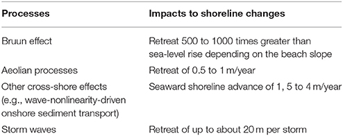
Table 1. Order of magnitude for cross-shore sedimentary processes contributing to shoreline change for typical coastal settings in the Netherlands and Australia and for a closure depth of 10 m (data from Stive, 2004).

TABLE 2

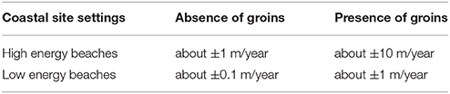
Table 2. Order of magnitude for the annual longshore sedimentary processes contributions to shoreline changes for typical coastal settings in the Netherlands and Australia and for a closure depth of 10 m (data from Stive, 2004).

The periods of time by which one will be able to (in)validate the use of Bruun rule in Equation (1) is a critical unknown. The question is complex, because all terms in Equation (1) are uncertain, and because the duration by which sea-level-rise-induced erosion is decipherable likely depends on climate change scenario and regional coastal settings. Ultimately, this effect might never be observed in some regions, if the impacts of sea-level rise remain smaller than those of other sedimentary processes causing shoreline change. To investigate this question, we consider the case of idealized wave-exposed sandy beaches with infinite sand availability, and we adapt an approach developed to quantify uncertainties in future flooding occurrence (Le Cozannet et al., 2015): we first define realistic probability density function for each uncertain parameter in Equation (1), using values from Stive (2004) and the IPCC (Church et al., 2013) (Section 2). In Section 3, we propagate these uncertainties through Equation (1) to provide shoreline change projections for different idealized coastal settings and climate change scenarios. Using a global sensitivity analysis (Sobol', 2001; Saltelli et al., 2008), we evaluate the contribution of each uncertain parameter to the variance of future shoreline changes. We use these results to assess where and when the Bruun effect should become observable. Finally, in Section 4, we discuss the results with respect to previous work and question the representativeness of the idealized sandy shorelines considered.

2. Materials and Methods

The method proceeds in three steps, which are detailed below.

2.1. Modeling Uncertainties of Input Parameters

We model the uncertainties of each input variable in Equation (1) using the probability density functions indicated in Table 3 and the values shown in Tables 1, 2. These tables consider different types of idealized coastal sites, based on the values provided by Stive (2004) for representative beaches in Australia and the Netherlands. For example, Table 2 indicates that if a groin extending far offshore is implemented on a high energy beach, it will act as a trap for the large longshore sediment transport and will contribute to shoreline change at a rate soundly exceeding 10 m/year. These orders of magnitudes can have a large site to site variability. This point is further discussed in the Section 5. Overall, in the absence of any other contribution similar to that of Stive (2004), we rely on the large uncertainties related to the contribution of each driving process shown in Tables 1, 2 to argue that they are applicable for a large number of sandy coasts.

TABLE 3

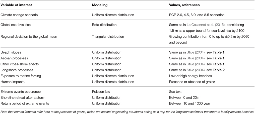
Table 3. Modeling of the different sources of uncertainties.

When defining probability distributions representing the uncertainties of input parameters (Table 3), the information available is often limited. As a general guidance, it should be avoided to introduce arbitrary constraints besides what is known already. In other words, the statistical entropy of the selected probability distribution functions should be maximized (Mishra, 2002). For example, a uniform probability density function should be selected when only boundaries are known. This case is met for most of the parameters given in Table 3, including the beach slopes and the contributions of cross-shore and longshore processes to the sedimentary budget. This choice reflects the fact that the data provided by Stive (2004) define boundary values for each uncertain input parameter (see Table 1).

More complex distribution can be elaborated when sufficient information is available. This is the case here for future sea-level rise. This source of uncertainties increases with time, and several components must be distinguished: (1) the selection of a climate change scenario, (2) the uncertainties of future sea-level rise for each climate change scenario, and (3) the regional variability of sea-level rise.

The IPCC provides likely range and median values for four climate change scenarios (RCP 2.6, 4.5, 6.0, and 8.5), corresponding to different trajectories of greenhouse gas emissions. To select one of these sets of value, we use a uniform discrete probability distribution, that is, a random application with a probability of 1∕4 to select each climate change scenario. This choice assumes that we do not know what will be future greenhouse gas emissions.

Even if the true climate change scenario was known, future sea-level rise would still remain uncertain, in particular because of insufficient knowledge on future ice-sheets melting and the Earth energy imbalance (Church et al., 2013; Kopp et al., 2014; von Schuckmann et al., 2016). Modeling results combined with expert judgements have suggested that this source of uncertainties can be adequately modeled by a skewed distribution with a finite support (Ben Abdallah et al., 2014; Jevrejeva et al., 2014). As in our previous article (Le Cozannet et al., 2015), we use a Beta distribution to represent this source of uncertainties. While many scientists estimate that the actual rates sea-level rise over the 21st century could exceed those anticipated by the IPCC (Horton et al., 2014), we strongly rely on their likely range and median values to elaborate our sea-level rise scenarios (Church et al., 2013). The upper bound of the distribution is a critical unknown, due to uncertainties in the dynamics of polar ice-sheets melting, which is currently accelerating (Rignot et al., 2011). Referring to recent modeling results of the Antarctic ice-sheet instability (Ritz et al., 2015), we use a conservative estimate of 1.5 m for the upper bound of sea-level rise by 2100. To our knowledge, there is presently no evidence that the low-probability and high impact event of an ice-sheet instability can be avoided, even for the climate change scenario RCP 2.6. Therefore, we use the same upper bound of 1.5m by 2100 for all climate change scenarii. This results in probabilistic sea-level rise scenarios as indicated in Figure 1.

FIGURE 1

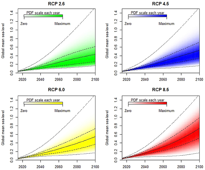
Figure 1. Probabilistic global sea-level rise projections used in this study. For each date, the intensity of the color represents the probability density function (PDF), and the solid and dashed black lines represent the median and likely ranges. The dotted lines represent the minimum and maximum values.

Due to spatially non-uniform warming of the ocean and the response of the Earth to ice-sheets melting, sea-level rise will display regional variability (Slangen et al., 2014a; Carson et al., 2016). This introduces an additional source of uncertainties. We assume that it includes a large part of natural randomness, which we evaluate using Church et al. (2013) and Carson et al. (2016). These references suggest that in addition to the boundaries of the distribution, its most likely value is known. Hence, the principle of maximum entropy leads to the choice of a triangular distribution (Mishra, 2002).

Extreme events are generated here assuming their occurrence follows a Poisson distribution. While this assumption is commonly used (Ranasinghe et al., 2012; Wainwright et al., 2015), it is challenged by some storm sequences, such as the winter 2013–2014 events in western Europe (Masselink et al., 2016). Moreover, as we use a Poisson distribution with fixed parameters, only the interannual variability of storms is captured, and the natural randomness is assumed unaffected by climate change (Plant et al., 2014). This hypothesis could be justified, as it is still difficult to assess where and to which extent climate change will affect extreme winds and waves (Planton et al., 2008; Mori et al., 2010; Hemer et al., 2013). However, we consider here that the return periods of storms are uncertain as well. The range of values considered for this uncertain input parameter is sufficiently large to exceed any plausible change of storminess due to climate change and any other limitation related to the Poisson assumption (see Table 1). Finally, we assume that the shoreline retreats after each extreme event ranges from 0 to 20 m. The first value can correspond to a storm occurring at low tide. Field surveys shows that the second value can result from a collision regime after exceptional storms, and can even be exceeded in case of overwash or breaching, which are not considered in this study. Figure 2 shows examples of shoreline retreats observed in western France after the storm Xynthia in February 2010 (Pedreros et al., 2010; Garcin et al., 2011). The return period of water levels for this storm is estimated to be approximately 200 year in the harbor of La Rochelle (Bulteau et al., 2015). Such return periods are consistent with our working hypothesis, and we note that shoreline retreat ranged from a few meters to 20 m, except where breach occurred. Similar values can be found in many other studies (e.g., Forbes et al., 2004; Mendoza and Jiménez, 2006; Roelvink et al., 2009; Loureiro et al., 2014).

FIGURE 2

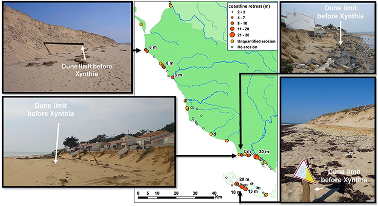
Figure 2. Field evidences of sandy beaches retreats of up to 20 m after the storm Xynthia in 2010 (Data: Pedreros et al., 2010; Garcin et al., 2011). The photographs present examples of indicators that allow to quantify the dune retreats. After this storm, the only retreat exceeding 20 m corresponds to a breaching event. Note that the return period of water levels in the harbor of La Rochelle is estimated at about 200 year for Xynthia (Bulteau et al., 2015), and is therefore compatible with the random sample of storms considered in this study.

As a summary, our approach relies on two major assumptions: (1) sea-level rise scenarios are based on IPCC; (2) we consider sites with gently sloping upper shorefaces, i.e., which are the most impacted by the Bruun effect. Other assumptions can be mentioned: some input parameters here are assumed independent, although they are not in practice. For example, for the same sediment size, beach slopes are expected to be steeper for low-energy beaches (Wright and Short, 1984). However, given the range of uncertainties provided in Table 3, such limitations can be left aside in a first attempt to propagate uncertainties through Equation (1).

2.2. Propagation of Uncertainties Through the Sediment Balance Equation

The second step of the approach consists in propagating these uncertainties through Equation (1).

The computational approach starts with defining auxiliary variables with uniform values in the interval [0,1]. Then we apply inverse cumulative distribution functions to these auxiliary variables, in order to generate distributions with the desired shapes (e.g., Beta distribution for sea-level rise). This computational approach ensures the independence of the different input parameters considered in Table 3, so that the Sobol' parameters (see next section) can be computed using a classical procedure. To reduce the computation time, we use a quasi-Monte-Carlo approach, where we assign values following a quasi-random Sobol' sequence (Sobol', 1967) to the auxiliary variables with values in [0,1]. We empirically determine the number of computations required to converge, by comparing purely random against quasi-random simulations in a test case corresponding to a situation of the end of the 21st century.

This procedure allows to produce generic probabilistic shoreline change projections based on the coastal tract assumptions. Importantly, all input parameters vary simultaneously during these simulations. Therefore, the probability density function of future shoreline change projections integrates the complete variability.

2.3. Quantifying and Ranking the Sources of Uncertainties in Shoreline Change Projections

Once uncertainties of all input parameters have been propagated through Equation (1), we obtain a distribution for future shoreline change as a function of time. To understand what this distribution means, we analyse the contribution of each uncertain input parameter to the variance of the model outcome using a global sensitivity analysis (Sobol', 2001; Saltelli et al., 2008).

The principle of variance-based global sensitivity analysis is to decompose the variance of the model outcome Y into several terms that relate to each uncertain input parameter X_i. These terms are called the Sobol' indices. Two subsets of terms are of particular interest for the evaluation of uncertainties: the first-oder and total order Sobol' indices.

The first-order Sobol' indices (S_i) correspond to the contribution of a given input parameter alone to the variance of the model outcome:

$\begin{array}{ll}{S}_i=\frac{Var(E(Y|X_i))}{Var(Y)}\hfill & (2)\hfill \end{array}$

They represent the expected proportion of the variance of the model outcome that would be removed if X_i was known.

The total order Sobol' index (S_Ti) represents the contribution of a given input parameter and all its interactions with other parameters to the variance of the model outcome. It is defined as:

$\begin{array}{ll}{S}_{Ti}=1-\frac{Var(E(Y|X_{-i}))}{Var(Y)}\hfill & (3)\hfill \end{array}$

with X_−i the set of all X_j except X_i. This index is used to identify which parameters can be set to any possible value without much impact to the variance of Y.

All computations are done using R (R Core Team, 2014), using the same quasi Monte-Carlo approach as in the previous section. The values of the Sobol' indices are very similar for two consecutive years. Therefore, to reduce the computing time, we calculate these indices each 5 year and interpolate them over the 21st century. We use the codes developped by the Joint Research Center of the European Commission to compute the first and total order Sobol' indices (see Jansen, 1999; Saltelli et al., 2010, for the related algorithms and formulations).

3. Results: When Will We be Able to (In)Validate the Bruun Rule?

Figure 3 shows the probabilistic shoreline change projections ΔS(t) at year t, once uncertainties from the input parameters (Table 3) have been propagated through Equation (1). This represents ΔS(t) if no prior information is available, besides values in Tables 1–3. Figures 4–6 show ΔS(t) for high and low energy beaches, with and without groins, and considering the different climate change scenarios separately.

FIGURE 3

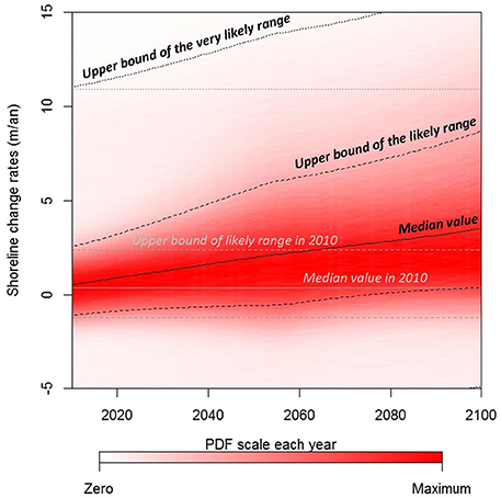
Figure 3. Shoreline retreat rate projections for the 21st century, with no prior information regarding the type of sandy coast considered, the impacts of man-made infrastructures and the climate change scenario. Positive values corresponds to shoreline retreat. For each date, the intensity of the color represents the probability density function, and the solid, dashed and dotted black lines represent the median, likely, and very likely ranges. The gray lines represent present days rates: they are extended toward the whole 21st century for comparison. They represent a virtual case in which sea-level remains at its present level, whereas the black lines take into account uncertain sea-level rise scenarios of Figure 1 using the Bruun rule.

FIGURE 4

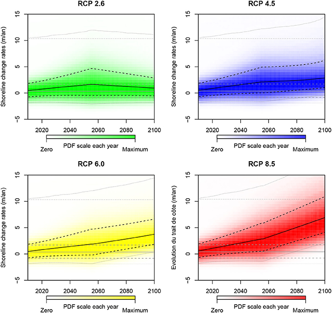
Figure 4. Shoreline change rate projections for the 21st century for high-energy sandy coasts with no impacts of man-made infrastructures and for different IPCC climate change scenarios. The same results are obtained for low-energy beaches with groins (see values of the contributions of longshore processes to the sedimentary budget in Table 2). The meaning of gray and black lines is the same as in Figure 3.

As expected, a slight shift toward erosion is observed over the 21st century (Figure 3). However, in practice, the response is very different depending on the climate change scenario and the type of coast considered. In case of RCP 2.6, we can not identify any clear separation between present and future probability density functions of shoreline change rates. Conversely, for other climate change scenarios and for beaches without groins, the likely range of future shoreline change rates separates or nearly separates (case of RCP 4.5) from present days values (Figures 4, 5). For example, in case of RCP 8.5 and coasts without groins, it is more than likely that observations will separate from their present values by the end of the 2060s for low-energy beaches, and in the early 2070s for high-energy beaches. Hence, using Figures 4, 5, it becomes possible to identify times of emergence for a more than likely observable shift toward erosion of sandy beaches under the assumptions listed above. As a practical implication, it should be possible to assess the Bruun rule validity by the mid-21st century on beaches without groins with gently sloping shoreface, if efforts to reduce greenhouse gas concentrations in the atmosphere fail.

FIGURE 5

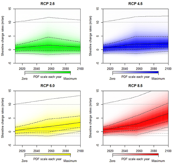
Figure 5. Shoreline change rate projections for the 21st century for low-energy sandy coasts with no impacts of man-made infrastructures and for different IPCC climate change scenarios. The meaning of gray and black lines is the same as in Figure 3.

If groins are present on the beach, the longshore processes have a larger impact on the sedimentary budget (Table 2): on the one hand, large volumes of sediments can be trapped in protected areas, but on the other hand, these sediments are missing in adjacent locations. This does not prevent from observing a shift toward erosion in case of low-energy beaches and climate change scenarios RCP 4.5, 6.0, and 8.5 (Figure 4). In these cases, not enough sediments can be trapped to compensate the losses induced by sea-level rise. Conversely, if groins are built on high-energy beaches, the transport of sediment is severely altered. This results in high variability of shoreline advance and retreat, reaching ±10 m/year (see Stive, 2004, and Table 2), which may compensate the impacts of sea-level rise theoretically (Figure 6). However, it is widely acknowledged that groins are not a sustainable solution because they typically fix the erosion issue, but shift it nearby. Hence, it should not be concluded that groins are an efficient adaptation strategy for high-energy sandy coasts.

FIGURE 6

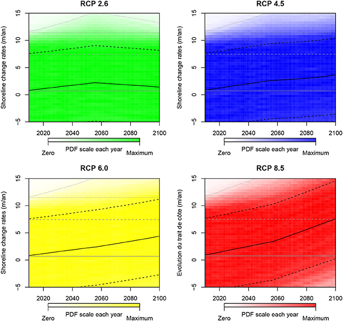
Figure 6. Shoreline change rate projections for the 21st century for high-energy sandy coasts with groins and for different IPCC climate change scenarios. The meaning of gray and black lines is the same as in Figure 3.

Drawing on these results, present day and future rates of shoreline change could remain indistinguishable if greenhouse gas emissions are reduced importantly (RCP 2.6 scenario). In addition, for coastal sites similar to those presented by Stive (2004), the times of emergence of a shift toward erosion induced by sea-level rise should occur during the second half of the 21st century, if sea-level rise follows the IPCC projections.

4. Further Insights from the Global Sensitivity Analysis

Figure 3 reflects a situation where nothing is known regarding local coastal settings, future climate change and sea-level rise, except their probability density functions. To obtain this figure, 12 uncertain parameters were propagated in Equation (1), resulting in shoreline change projections with very large uncertainties. Indeed, the standard deviation of shoreline change projections rises from about 4 m/year now, to 4.5 m/year by 2050 and 5 m/year by 2100. These values are large, and the true values might be closer to 1 m/year (Bird, 1985). This suggests that the uncertainties in shoreline change projections can be reduced importantly with more knowledge regarding local coastal processes. Hence, the ensuing question is to understand what drives the variability of shoreline change projections in Figure 3. In this section, we investigate this issue using the results of the global sensitivity analysis. In other words, we separate the variance of ΔS(t) into several components corresponding to the contribution of the 12 uncertain input parameters, in order to gain further insight into the understanding of the upper shoreface sediment balance equation outcome under Table 3 constraints.

Figures 7, 8 show the first and total order Sobol' indices obtained by the global sensitivity analysis. Using these figures, it becomes possible to classify input parameters according to their contribution to the variability of shoreline change rates: the first order Sobol' indices are used to rank input parameters, whereas the variability of parameters with total order Sobol' indices close to zero can be neglected without much impacts to the variability of the final results (Saltelli, 2004). In the following subsections, the uncertain input parameters of Equation (1) are classified according to their first and total order Sobol' indices, which reveal research priorities to better anticipate future shoreline change under the Bruun rule assumption.

FIGURE 7

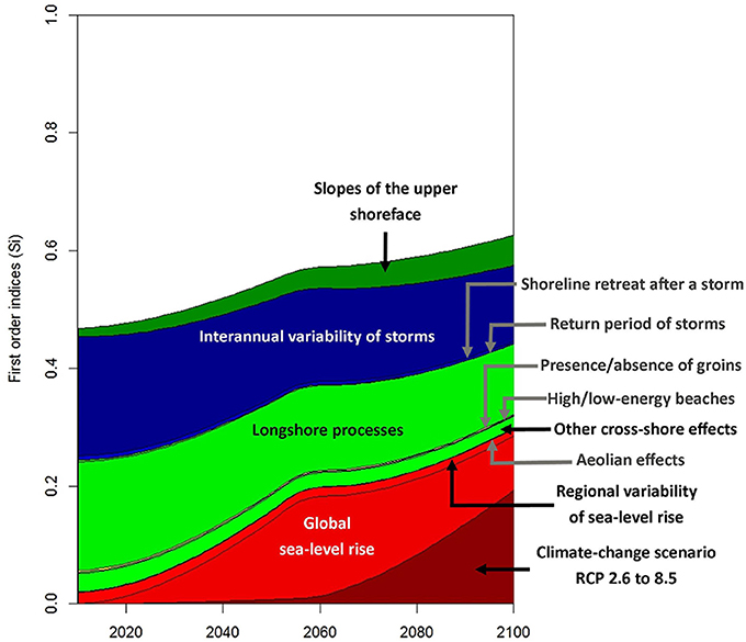
Figure 7. Evolution of the first order Sobol' indices over the time, indicating the contribution of each varying parameter alone to the final uncertainty. Parameters indicated in gray have the smallest 1st order Sobol' indices. The inflexion of the curves after 2060 is due to two phenomena: first, the different climate change scenarios (RCP 2.6–8.5) induce different sea-level rise projections by that time (see Figure 1); second, shoreline change projections uncertainties by 2100 is much larger by 2100 than now (see text). The colors (red, green, blue, and yellow) indicate uncertainties related to (1) climate change and sea-level rise, (2) local site characteristics, (3) impacts of storms, and (4) of coastal defenses (groins).

FIGURE 8

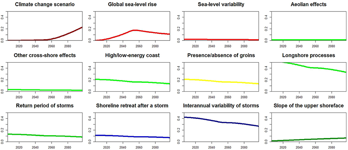
Figure 8. Evolution of the total order Sobol' indices over the time, indicating which parameter can be fixed to any possible values without much impact to the variance of the model outcome. Please refer also to the legend of Figure 7 for explanations on the colors and inflexions of the curves.

4.1. Critical Unknowns for the Present Days

The random variables used to model the interannual variability of storms and the impacts of longshore sedimentary processes display large first and total order indices: Figure 7 shows that the value of the first order indices is of about 0.2. Figure 7 indicates that the total order indices decreases from about 0.6–0.3 for longshore processes (0.4–0.3 for the interannual variability of storms). Therefore, these parameters account for a large part of the uncertainties in shoreline change projections. As a consequence, knowing more about these processes should be a priority for reducing the uncertainties resulting from the application of the sediment balance equation for sandy upper shorefaces with gentle slopes. For example, our results implies that a perfect knowledge of longshore processes would reduce the variance of shoreline change projections by a factor of nearly 20%. Many studies in the field of coastal research have studied these sources of uncertainties (Allen, 1981; Inman and Dolan, 1989; Slott et al., 2006; Roelvink et al., 2009; Castelle et al., 2015). However, it remains difficult to quantify precisely all the phenomena involved (see Section 5). Here, the results of the global sensitivity analysis just highlight that sandy shoreline change projections are more accurate if the impacts of storms and longshore sedimentary processes are taken into account. While integrating these processes at regional to global scales is a challenge, it is increasingly addressed in recent assessments of climate change impacts (e.g., Anderson et al., 2015).

4.2. Uncertain Parameters with Minor Impacts

At the opposite, the Sobol' first and total order indices representing the aeolian processes, other cross-shore effects (e.g., due to waves asymmetry) and the regional variability of sea-level rise are small. Therefore, the variability of these parameters can be neglected without any large impact to the variability of shoreline change projections. This result can seem surprising. In fact, several studies have highlighted the importance of cross-shore sedimentary processes in explaining seasonal and interannual shoreline changes (e.g., Yates et al., 2009; Splinter et al., 2014). To understand how our results can be related to these findings, we need to point out that Stive (2004) distinguishes the rapid erosive impacts of highly energetic events from the slow accretion due to the net onshore contributions from mild waves (Table 1).

The regional variability of sea-level rise also plays a minor role, whereas it can be much more important for strongly non-linear impact models. For example, urban coastal flooding generally becomes most damaging once a critical threshold has been exceeded (Hallegatte et al., 2013; Idier et al., 2013b; Miller et al., 2014). In this case, knowing more about the regional variability of sea-level rise would be one of the priorities for coastal managers interested in understanding how risk will evolve over the coming decades (Le Cozannet et al., 2015).

According to Table 1, aeolian processes taking place on coastal beaches and dunes are expected to induce net sediment losses and shoreline retreat. However, these processes do not appear as a critical unknown either, in spite of their complexity (Arens, 1996; Hesp et al., 2013; Bauer et al., 2015). Again, our results highlight that when few data are available regarding other coastal processes, the values provided in Table 1 are sufficiently narrow to anticipate the impacts of the slow recovery of beaches satisfactorily. Finally, as this result comes directly from the order of magnitude provided in Tables 1–3, it can be invalidated if new observations demonstrate that these processes have much larger impacts. This question of the representativeness of the values of Tables 1, 2 is addressed in details in the discussion section.

4.3. Interactions between Processes: Why is a Global Sensitivity Analysis Recommended?

Figures 7, 8 also reveal that for two random variables, the Sobol' first order indices are close to zero, whereas the total order indices are large. This is the case for example for the random variables indicating if groins are built on the beach, or if the beach is exposed to low- or high- energetic conditions: their total order Sobol' indices ranges from 0.1 to 0.2 (Figure 8). In this case, the principles of the global sensitivity analysis implies that the variability of the input parameters cannot be neglected, because it interacts with other random variables (Saltelli, 2004). In other words, this result indicates that, for instance, groins will have little impacts on shoreline change if longshore drift is weak.

Figure 7 shows that the sum of the first order Sobol' indices ranges from 0.45 to 0.6 depending on the period of time considered. This means that the interaction term is large. Hence, to a significant extent, the overall variability is driven by the combined variation of the parameters (joint effect). A very common way to perform a sensitivity analysis consists in evaluating the model response to each uncertain input factor independently. Our results show that despite the apparent simplicity of Equation (1), such an approach could fail to rank the impact of each uncertainty source: the total uncertainty on shoreline change can not be considered as the sum related to each uncertainty sources taken alone. On the contrary, the combined effect among them should be accounted for: here the interaction terms represent about the half of the total variance of shoreline change projections.

4.4. Critical Unknowns for the Next Decades

Figures 7, 8 shows two distinct periods, during which the relative importance of sea-level rise, climate change scenarios, and beach slopes increase successively. This result primarily comes from the propagation of uncertain sea-level rise scenarios (Figure 1) in the Bruun term of Equation (1).

First, the climate change scenarios have small Sobol' indices during the 1st part of the 21st century. Therefore, as expected, the next decades do not appear as a relevant period of time to differentiate future shoreline change according to the future climate change scenarios. However, sea-level will be rising, and Equation (1) implies that this will induce a slight shift toward erosion. By 2050, uncertainties on global sea-level rise account for 20% of the variance of future shoreline change projections.

Conversely, there are large differences between e.g., RCP 2.6 and RCP 8.5 during the second part of the 21st century. Figure 7 shows that if a decision is taken to follow a given climate change scenario, the variance of shoreline change projections is reduced by 20%. This is almost twice the maximum reduction of variance that we could expect, if we were able to predict accurately future sea-level rise given greenhouse gas emissions by 2100. Hence, even if nothing is known regarding coastal processes besides Table 1, the benefits of climate change mitigation and greenhouse gaz emissions reductions appear significant, as suggested by Nicholls and Lowe (2004) and Pardaens et al. (2011). Here, Figures 7, 8 constitute an other way to communicate this result, which was already identified in Section 3 and Figure 3.

4.5. Appropriate Coastal Settings for Validating the Use of the Bruun Rule in the Sediment Budget Equation

Figures 3–6 have indicated that if a large number of coastal sites are considered, (in)validating the use of the Bruun rule in Equation (1) will be straightforward by the end of the 21st century for RCP 6.0 and 8.5 scenarios (see Section 3). In a more general case, the results of the global sensitivity analysis (Figures 7, 8) enable to identify which types of coastal sites are potential candidates for testing the use of the Bruun term in Equation (1): beaches without human impacts, little exposed to storms and where longshore drift can be quantified are among such sites. This result is not a surprise: previous studies that tried to validate the Bruun rule and detect an observable impact of sea-level rise on shoreline change actually focused precisely on this type of coasts (Leatherman et al., 2000b; Zhang et al., 2004). In practice however, the selection of such sites is not straightforward, and there remains question regarding the possibility to remove the impacts of longshore drift in the analysis (Leatherman et al., 2000a; Sallenger et al., 2000). Nevertheless, these results provide a perspective for coastal observatories currently collecting coastal evolution observations with the aim of better understanding coastal impacts of climate change.

5. Discussion: Representativeness of the Selected Idealized Coastal Sites

Our study relies on the orders of magnitudes provided by Stive (2004) for typical coastal settings in the Netherlands and Australia. Though there is no study providing orders of magnitude at other representative sites, it is hypothesized that the respective contribution of each process in Tables 1, 2 vary considerably for other coastal settings. For instance, on open and straight sandy beaches exposed to high-energy oblique ocean waves, longshore sediment transport rate can be high [e.g., O(10⁶ m³/year)] but without any alongshore gradients. In such a situation, longshore sedimentary processes do not contribute to shoreline change. This is the case of the southern Gironde Coast, SW France, where gradients in longshore sediment transport are negligible (Idier et al., 2013a) and where the observed shoreline variability on the timescales from hours to years can be explained by cross-shore processes only (Castelle et al., 2014). Yet, even in this simplified coastal setting, there is to date no detailed quantification of the contribution of aeolian processes and other cross-shore processes to the overall shoreline change. As far as extreme storms are concerned, it is impossible to quantify maximum storm wave erosion for given return period exceeding a few decades simply because there is no such long time series of storm-driven erosion. At the same beach, the cumulative impact of a series of outstanding storms during the winter 2013/2014 only drove a 15 m dune retreat over 3 months (Castelle et al., 2015). The same outstanding severe storms drove highly variable erosion patterns along Western Europe (Masselink et al., 2016), revealing the complexity of quantifying the erosion driven by multi-decadal or multi-centennial return period storms.

While providing numbers for this simple case of open beaches with no alongshore sediment transport gradients is arguably challenging, this is even worst for embayed beaches. Embayed beaches are ubiquitous worldwide given that nearly half of the world's coast consists of hilly or mountainous coastline. In addition, beaches artificially bounded by groins or jetty can behave as embayed beaches. Shoreline variability along embayed beaches is dominated by rotation signal (Ranasinghe et al., 2004). However, the respective contributions of cross-shore and longshore processes to the embayed beach rotation signal is still a subject of debate (Ranasinghe et al., 2004; Harley et al., 2011, 2015).

Overall, although we do not pretend to address all sandy coasts worldwide, we advocate that the values given by Stive (2004) are sufficiently large to be representative of many coastal settings. It is obvious that further work is required (1) to decipher the respective contributions of the different driving processes to shoreline change in different coastal settings and (2) to develop alternative model framework in which the different processes can be accounted for explicitly. In this framework, reduced-complexity modeling approaches (e.g., Splinter et al., 2014; Reeve et al., 2015) appear as a relevant avenue.

Noteworthy, Stive (2004) refers to coastal sites with gentle slopes, ranging from 0.001 to 0.002, which corresponds to very gentle slopes actually (Hinton and Nicholls, 1998; Marsh et al., 1998). Shoreface slopes are often larger. For instance in SW France, high-energy beaches display coastal slopes of about 0.015 (Castelle et al., 2014), whereas they reach about 0.012 for low-energy Mediterranean beaches in Languedoc (Yates et al., 2011). In practice, however, the use of the Bruun rule in Equation (1) is more questionable for steep coasts. Other models would be required in such coastal sites, for example considering the sediment losses and gains during and after each storm (Larson et al., 2004; Ranasinghe et al., 2012). Nevertheless, we acknowledge that beach slopes values that can be calculated from Table 3 correspond to coastal sites where the Bruun effect will have the strongest impacts.

The approach presented here could be applied to other medium-complexity geomorphic evolution modeling approaches (French et al., 2015), in order to finally identify research priorities. However, in the case of complex coastal settings with limited sand availability, the constraints imposed by the geology, the continental sedimentary supply or the role of coastal lagoons should be considered as well.

6. Conclusion

In this article, we examined where and by which period of time the Bruun effect should become observable on wave-exposed sandy coasts. To do this, we refered to Stive (2004) to evaluate the order of magnitude of each physical process contributing to shoreline change in the case of coastal upper-shoreface with gentle slopes. We also considered probabilistic sea-level rise scenarios based on the IPCC (Church et al., 2013). We propagated these uncertainties through the sediment balance equation, that sums the Bruun effect with other drivers such as longshore and cross-shore processes. This allowed to identify a time of emergence of an observable Bruun effect by the middle of the 21st century in the case of beaches with gentle slopes without groins, and for climate change scenarios RCP 4.5, 6.0, and 8.5 only. Under the assumptions above, the absence of generalized sea-level-rise-driven beach erosion by the end of the 21st century is only achieved for RCP 2.6 climate change scenario.

Rather than predictions of future shoreline changes, our results can be viewed as an attempt to better understand where and when the Bruun rule can be (in)validated. Using a global sensitivity analysis, our results confirm that low-energy gently sloping beaches with little human impacts and small gradients in longshore drift and sheltered from storms are the most relevant to assess the validity of the Bruun rule in the sediment balance equation. These results could be further improved through a better integration of the primary driving processes of shoreline change in the sediment balance equation, and refined probability distribution functions. This also implies collecting site-specific and more accurate values than those listed in Tables 1, 2. Whatever the amount of data collected, part of the uncertainties in future shoreline change projections will remain. In addition, it should be noted that new knowledge may also illuminate some “not-yet envisaged” complex processes, of which our understanding may still be poor, and would require new research efforts in the future. Overall, and regardless the shortcomings discussed above, our approach is a relevant modeling framework to further improve communication to stakeholders and general public on uncertainties in sea-level rise impact assessments.

Author Contributions

Overall design of the study: GC. Detailed design and implementation of the study: GC, CO, BC, MG, DI, RP, JR. Interpretation and discussion: All. Writing and correcting the paper: All.

Conflict of Interest Statement

The authors declare that the research was conducted in the absence of any commercial or financial relationships that could be construed as a potential conflict of interest.

Acknowledgments

This project has been funded by BRGM through the “Adaptation to Climate Change Risks” project. BC was funded by the CHIPO project (ANR-14-ASTR-0004-01), financially supported by the Agence Nationale de la Recherche (ANR). The field mission following Xynthia (Figure 2) was funded by BRGM, and conducted by MG and RP, Daniel Monfort, Julie Mugica, Yann Krien, and Benjamin Francois. We thank Thomas Bulteau, Anny Cazenave, Franck Desmazes, Franck Lavigne, Cesca Ribas, and Marcel Stive for useful discussions and comments that finally resulted in this study. Finally, we thank the two reviewers for their very useful comments.

References

Aagaard, T., and Sørensen, P. (2013). Sea level rise and the sediment budget of an eroding barrier on the danish North sea coast. J. Coast. Res. SI65, 434–439. doi: 10.2112/SI65-074.1

CrossRef Full Text | Google Scholar

Allen, J. R. (1981). Beach erosion as a function of variations in the sediment budget, Sandy-Hook, New-Jersey, USA. Earth Surf. Process. Land. 6, 139–150.

Google Scholar

Anderson, T. R., Fletcher, C. H., Barbee, M. M., Frazer, L. N., and Romine, B. M. (2015). Doubling of coastal erosion under rising sea level by mid-century in Hawaii. Nat. Hazards 78, 75–103. doi: 10.1007/s11069-015-1698-6

CrossRef Full Text | Google Scholar

Arens, S. (1996). Patterns of sand transport on vegetated foredunes. Geomorphology 17, 339–350.

Google Scholar

Bauer, B. O., Hesp, P. A., Walker, I. J., and Davidson-Arnott, R. G. (2015). Sediment transport (dis)continuity across a beach–dune profile during an offshore wind event. Geomorphology 245, 135–148. doi: 10.1016/j.geomorph.2015.05.004

CrossRef Full Text | Google Scholar

Ben Abdallah, N., Mouhous-Voyneau, N., and Denoeux, T. (2014). Combining statistical and expert evidence using belief functions: application to centennial sea level estimation taking into account climate change. Int. J. Approx. Reason. 55, 341–354. doi: 10.1016/j.ijar.2013.03.008

CrossRef Full Text | Google Scholar

Bird, E. (1985). Coastal Changes: A Global Review. New York, NY: Wiley.

Bruun, P. (1962). Sea-level rise as a cause of shore erosion. J. Waterway. Harbour. Div. 88, 117–130.

Bulteau, T., Idier, D., Lambert, J., and Garcin, M. (2015). How historical information can improve estimation and prediction of extreme coastal water levels: application to the Xynthia event at La Rochelle (france). Nat. Hazards Earth Syst. Sci. 15, 1135–1147. doi: 10.5194/nhess-15-1135-2015

CrossRef Full Text

Carson, M., Köhl, A., Stammer, D., Slangen, A., Katsman, C., van de Wal, R., et al. (2016). Coastal sea level changes: observed and projected during the 20th and 21st century. Clim. Change 134, 269–281. doi: 10.1007/s10584-015-1520-1

CrossRef Full Text | Google Scholar

Castelle, B., Marieu, V., Bujan, S., Ferreira, S., Parisot, J.-P., Capo, S., et al. (2014). Equilibrium shoreline modelling of a high-energy meso-macrotidal multiple-barred beach. Mar. Geol. 347, 85–94. doi: 10.1016/j.margeo.2013.11.003

CrossRef Full Text | Google Scholar

Castelle, B., Marieu, V., Bujan, S., Splinter, K. D., Robinet, A., Sénéchal, N., et al. (2015). Impact of the winter 2013–2014 series of severe western europe storms on a double-barred sandy coast: Beach and dune erosion and megacusp embayments. Geomorphology 238, 135–148. doi: 10.1016/j.geomorph.2015.03.006

CrossRef Full Text | Google Scholar

Church, J., Clark, P., Cazenave, A., Gregory, J., Jevrejeva, S., Merrifield, M., et al. (2013). Sea Level Change. Climate Change 2013: The Physical Science Basis. Contribution of Working Group I to the Fifth Assessment Report of the Intergovernmental Panel on Climate Change. (Cambridge, UK; New York, NY: Cambridge University Press), 1137–1216.

Google Scholar

Cooper, J. A. G., and Pilkey, O. H. (2004). Longshore drift: trapped in an expected universe. J. Sediment. Res. 74, 599–606. doi: 10.1306/022204740599

CrossRef Full Text | Google Scholar

Cowell, P. J., Stive, M. J., Niedoroda, A. W., de Vriend, H. J., Swift, D. J., Kaminsky, G. M., et al. (2003a). The coastal-tract (part 1): a conceptual approach to aggregated modeling of low-order coastal change. J. Coast. Res. 19, 812–827.

Google Scholar

Cowell, P. J., Stive, M. J., Niedoroda, A. W., Swift, D. J., de Vriend, H. J., Buijsman, M. C., et al. (2003b). The coastal-tract (part 2): applications of aggregated modeling of lower-order coastal change. J. Coast. Res. 19, 828–848.

Google Scholar

Dangendorf, S., Marcos, M., Müller, A., Zorita, E., Riva, R., Berk, K., et al. (2015). Detecting anthropogenic footprints in sea level rise. Nat. Commun. 6:7849. doi: 10.1038/ncomms8849

PubMed Abstract | CrossRef Full Text | Google Scholar

Davidson-Arnott, R. G. (2005). Conceptual model of the effects of sea level rise on sandy coasts. J. Coast. Res. 21, 1166–1172. doi: 10.2112/03-0051.1

CrossRef Full Text | Google Scholar

Forbes, D. L., Parkes, G. S., Manson, G. K., and Ketch, L. A. (2004). Storms and shoreline retreat in the southern gulf of St. Lawrence. Mar. Geol. 210, 169–204. doi: 10.1016/j.margeo.2004.05.009

CrossRef Full Text | Google Scholar

French, J., Payo, A., Murray, B., Orford, J., Eliot, M., and Cowell, P. (2015). Appropriate complexity for the prediction of coastal and estuarine geomorphic behaviour at decadal to centennial scales. Geomorphology 256, 3–16. doi: 10.1016/j.geomorph.2015.10.005

CrossRef Full Text | Google Scholar

Garcin, M., Pedreros, R., Krien, Y., Monfort, D., Mujica, J., and Francois, B. (2011). Base de données d'observations de la Tempete Xynthia Sur le Littoral. Technical Report, BRGM. rapport BRGM/RP-59395-FR.

Golledge, N., Kowalewski, D., Naish, T., Levy, R., Fogwill, C., and Gasson, E. (2015). The multi-millennial Antarctic commitment to future sea-level rise. Nature 526, 421–425. doi: 10.1038/nature15706

PubMed Abstract | CrossRef Full Text | Google Scholar

Hallegatte, S., Green, C., Nicholls, R. J., and Corfee-Morlot, J. (2013). Future flood losses in major coastal cities. Nat. Clim. Change 3, 802–806. doi: 10.1038/nclimate1979

CrossRef Full Text | Google Scholar

Hansen, J., Sato, M., Hearty, P., Ruedy, R., Kelley, M., Masson-Delmotte, V., et al. (2015). Ice melt, sea level rise and superstorms: evidence from paleoclimate data, climate modeling, and modern observations that 2°C global warming is highly dangerous. Atmos. Chem. Phys. Discus. 15, 20059–20179. doi: 10.5194/acpd-15-20059-2015

CrossRef Full Text | Google Scholar

Harley, M., Turner, I., and Short, A. (2015). New insights into embayed beach rotation: the importance of wave exposure and cross-shore processes. J. Geophys. Res. Earth Surf. 120, 1470–1484. doi: 10.1002/2014JF003390

CrossRef Full Text | Google Scholar

Harley, M., Turner, I., Short, A., and Ranasinghe, R. (2011). A reevaluation of coastal embayment rotation: the dominance of cross-shore versus alongshore sediment transport processes, collaroy-narrabeen beach, southeast Australia. J. Geophys. Res. Earth Surf. 116:F04033. doi: 10.1029/2011JF001989

CrossRef Full Text | Google Scholar

Hemer, M. A., Fan, Y., Mori, N., Semedo, A., and Wang, X. L. (2013). Projected changes in wave climate from a multi-model ensemble. Nat. Clim. Change 3, 471–476. doi: 10.1038/nclimate1791

CrossRef Full Text | Google Scholar

Hesp, P. A., Walker, I. J., Chapman, C., Davidson-Arnott, R., and Bauer, B. O. (2013). Aeolian dynamics over a coastal foredune, Prince Edward island, Canada. Earth Surf. Process. Land. 38, 1566–1575. doi: 10.1002/esp.3444

CrossRef Full Text | Google Scholar

Hinkel, J., Nicholls, R. J., Tol, R. S., Wang, Z. B., Hamilton, J. M., Boot, G., et al. (2013). A global analysis of erosion of sandy beaches and sea-level rise: an application of DIVA. Glob. Planet. Change 111, 150–158. doi: 10.1016/j.gloplacha.2013.09.002

CrossRef Full Text | Google Scholar

Hinton, C., and Nicholls, R. J. (1998). Spatial and temportal behavior of depth of closure along the Holland coast. Coast. Eng. Proc. 1, 2913–2925. doi: 10.1061/9780784404119.221

CrossRef Full Text | Google Scholar

Horton, B. P., Rahmstorf, S., Engelhart, S. E., and Kemp, A. C. (2014). Expert assessment of sea-level rise by ad 2100 and ad 2300. Q. Sci. Rev. 84, 1–6. doi: 10.1016/j.quascirev.2013.11.002

CrossRef Full Text | Google Scholar

Idier, D., Castelle, B., Charles, E., and Mallet, C. (2013a). Longshore sediment flux hindcast: spatio-temporal variability along the sw atlantic coast of France. J. Coast. Res. 2, 1785. doi: 10.2112/SI65-302.1

CrossRef Full Text | Google Scholar

Idier, D., Rohmer, J., Bulteau, T., and Delvallée, E. (2013b). Development of an inverse method for coastal risk management. Nat. Hazards Earth Syst. Sci. 13, 999–1013. doi: 10.5194/nhess-13-999-2013

CrossRef Full Text | Google Scholar

Inman, D. L., and Dolan, R. (1989). The outer banks of North-Carolina - budget of sediment and inlet dynamics along a migrating barrier system. J. Coast. Res. 5, 193–237.

Google Scholar

Jansen, M. J. (1999). Analysis of variance designs for model output. Comput. Phys. Commun. 117, 35–43.

Google Scholar

Jevrejeva, S., Grinsted, A., and Moore, J. C. (2014). Upper limit for sea level projections by 2100. Environ. Res. Lett. 9:104008. doi: 10.1088/1748-9326/9/10/104008

CrossRef Full Text | Google Scholar

Kopp, R. E., Horton, R. M., Little, C. M., Mitrovica, J. X., Oppenheimer, M., Rasmussen, D. J., et al. (2014). Probabilistic 21st and 22nd century sea-level projections at a global network of tide-gauge sites. Earth Future 2, 383–406. doi: 10.1002/2014EF000239

CrossRef Full Text | Google Scholar

Larson, M., Erikson, L., and Hanson, H. (2004). An analytical model to predict dune erosion due to wave impact. Coast. Eng. 51, 675–696. doi: 10.1016/j.coastaleng.2004.07.003

CrossRef Full Text | Google Scholar

Le Cozannet, G., Garcin, M., Yates, M., Idier, D., and Meyssignac, B. (2014). Approaches to evaluate the recent impacts of sea-level rise on shoreline changes. Earth Sci. Rev. 138, 47–60. doi: 10.1016/j.earscirev.2014.08.005

CrossRef Full Text | Google Scholar

Le Cozannet, G., Rohmer, J., Cazenave, A., Idier, D., Van de Wal, R., De Winter, R., et al. (2015). Evaluating uncertainties of future marine flooding occurrence as sea-level rises. Environ. Model. Softw. 73, 44–56. doi: 10.1016/j.envsoft.2015.07.021

CrossRef Full Text | Google Scholar

Leatherman, S. P., Zhang, K., and Douglas, B. C. (2000a). Reply to comment on sea level rise shown to drive coastal erosion. Eos Trans. Am. Geophys. Union 81, 437–441. doi: 10.1029/00EO00330

CrossRef Full Text | Google Scholar

Leatherman, S. P., Zhang, K., and Douglas, B. C. (2000b). Sea level rise shown to drive coastal erosion. Eos Trans. Am. Geophys. Union 81, 55–57. doi: 10.1029/00EO00034

CrossRef Full Text | Google Scholar

Loureiro, C., Ferreira, Ó., and Cooper, J. A. G. (2014). Non-uniformity of storm impacts on three high-energy embayed beaches. J. Coast. Res. 70, 326–331. doi: 10.2112/SI70-055.1

CrossRef Full Text | Google Scholar

Marcos, M., Tsimplis, M. N., and Shaw, A. G. (2009). Sea level extremes in southern Europe. J. Geophys. Res. Oceans 114:C01007. doi: 10.1029/2008jc004912

CrossRef Full Text | Google Scholar

Marsh, S., Nicholls, R., Kroon, A., and Hoekstra, P. (1998). Assessment of depth of closure on a nourished beach: Terschelling, the Netherlands. Coast. Eng. Proc. 1, 3110–3123. doi: 10.1061/9780784404119.236

CrossRef Full Text | Google Scholar

Masselink, G., Castelle, B., Scott, T., Dodet, G., Suanez, S., Jackson, D., et al. (2016). Extreme wave activity during winter 2013/2014 and morphological impacts along the atlantic coast of Europe. Geophys. Res. Lett. 45, 2135–2143. doi: 10.1002/2015GL067492

CrossRef Full Text | Google Scholar

Mendoza, E. T., and Jiménez, J. A. (2006). “Storm-induced beach erosion potential on the catalonian coast,” in Journal of Coastal Research, Proceedings of the 3rd Spanish Conference on Coastal Geomorphology (Spain: Coastal Education & Research Foundation, Inc.), 81–88.

Google Scholar

Menéndez, M., and Woodworth, P. L. (2010). Changes in extreme high water levels based on a quasi-global tide-gauge data set. J. Geophys. Res. Oceans 115:C10011. doi: 10.1029/2009jc005997

CrossRef Full Text | Google Scholar

Miller, A., Jonkman, S. N., and Van Ledden, M. (2014). Risk to life due to flooding in post-Katrina New-Orleans. Nat. Hazards Earth Syst. Sci. Discus. 2, 825–864. doi: 10.5194/nhessd-2-825-2014

CrossRef Full Text | Google Scholar

Mishra, S. (2002). Assigning Probability Distributions to Input Parameters of Performance Assessment Models. Stockholm: SKB.

Google Scholar

Mori, N., Yasuda, T., Mase, H., Tom, T., and Oku, Y. (2010). Projection of extreme wave climate change under global warming. Hydrol. Res. Lett. 4, 15–19. doi: 10.3178/hrl.4.15

CrossRef Full Text | Google Scholar

Nicholls, R. J., and Cazenave, A. (2010). Sea-level rise and its impact on coastal zones. Science 328, 1517–1520. doi: 10.1126/science.1185782

PubMed Abstract | CrossRef Full Text | Google Scholar

Nicholls, R. J., and Lowe, J. A. (2004). Benefits of mitigation of climate change for coastal areas. Glob. Environ. Change 14, 229–244. doi: 10.1016/j.gloenvcha.2004.04.005

CrossRef Full Text | Google Scholar

Pardaens, A., Lowe, J., Brown, S., Nicholls, R., and De Gusmâo, D. (2011). Sea-level rise and impacts projections under a future scenario with large greenhouse gas emission reductions. Geophys. Res. Lett. 38:L12604. doi: 10.1029/2011gl047678

CrossRef Full Text | Google Scholar

Passeri, D. L., Hagen, S. C., Medeiros, S. C., Bilskie, M. V., Alizad, K., and Wang, D. (2015). The dynamic effects of sea level rise on low gradient coastal landscapes: a review. Earth Future 3, 159–181. doi: 10.1002/2015EF000298

CrossRef Full Text | Google Scholar

Pedreros, R., Garcin, M., Monfort, D., and Krien, Y. (2010). Tempete Xynthia: Compte Rendu de Mission Préliminaire. Technical Report, BRGM. rapport BRGM/RP-58261-FR.

Plant, N. G., Flocks, J., Stockdon, H. F., Long, J. W., Guy, K., Thompson, D. M., et al. (2014). Predictions of barrier island berm evolution in a time-varying storm climatology. J. Geophys. Res. Earth Surf. 119, 300–316. doi: 10.1002/2013JF002871

CrossRef Full Text | Google Scholar

Planton, S., Déqué, M., Chauvin, F., and Terray, L. (2008). Expected impacts of climate change on extreme climate events. Comptes Rendus Geosci. 340, 564–574. doi: 10.1016/j.crte.2008.07.009

CrossRef Full Text | Google Scholar

R Core Team (2014). R: A Language and Environment for Statistical Computing. Vienna: R Foundation for Statistical Computing.

Ranasinghe, R., Callaghan, D., and Stive, M. J. F. (2012). Estimating coastal recession due to sea level rise: beyond the bruun rule. Clim. Change 110, 561–574. doi: 10.1007/s10584-011-0107-8

CrossRef Full Text | Google Scholar

Ranasinghe, R., McLoughlin, R., Short, A., and Symonds, G. (2004). The southern oscillation index, wave climate, and beach rotation. Mar. Geol. 204, 273–287. doi: 10.1016/S0025-3227(04)00002-7

CrossRef Full Text | Google Scholar

Ranasinghe, R., and Stive, M. J. F. (2009). Rising seas and retreating coastlines. Clim. Change 97, 465–468. doi: 10.1007/s10584-009-9593-3

CrossRef Full Text | Google Scholar

Reeve, D. E., Karunarathna, H., Pan, S., Horrillo-Caraballo, J. M., Różyński, G., and Ranasinghe, R. (2015). Data-driven and hybrid coastal morphological prediction methods for mesoscale forecasting. Geomorphology 256, 49–67. doi: 10.1016/j.geomorph.2015.10.016

CrossRef Full Text | Google Scholar

Rignot, E., Velicogna, I., Van den Broeke, M., Monaghan, A., and Lenaerts, J. (2011). Acceleration of the contribution of the Greenland and Antarctic ice sheets to sea level rise. Geophys. Res. Lett. 38:L05503. doi: 10.1029/2011gl046583

CrossRef Full Text | Google Scholar

Ritz, C., Edwards, T. L., Durand, G., Payne, A. J., Peyaud, V., and Hindmarsh, R. C. A. (2015). Potential sea-level rise from Antarctic ice-sheet instability constrained by observations. Nature 528, 115–118. doi: 10.1038/nature16147

PubMed Abstract | CrossRef Full Text | Google Scholar

Roelvink, D., Reniers, A., van Dongeren, A., de Vries, J. v. T., McCall, R., and Lescinski, J. (2009). Modelling storm impacts on beaches, dunes and barrier islands. Coast. Eng. 56, 1133–1152. doi: 10.1016/j.coastaleng.2009.08.006

CrossRef Full Text | Google Scholar

Sallenger, A. H., Morton, R., Fletcher, C., Thieler, E. R., and Howd, P. (2000). Comment on sea level rise shown to drive coastal erosion. Eos Trans. Am. Geophys. Union 81, 436–436. doi: 10.1029/EO081i038p00436-02

CrossRef Full Text

Saltelli, A. (2004). “Global sensitivity analysis: an introduction,” in Proceedings of the 4th International Conference on Sensitivity Analysis of Model Output (SAMO'04) (Los Alamos, NM), 27–43.

Google Scholar

Saltelli, A., Annoni, P., Azzini, I., Francesca Campolongo, Ratto, M., and Tarantola, S. (2010). Variance based sensitivity analysis of model output. design and estimator for the total sensitivity index. Comput. Phys. Commun. 181, 259–270. doi: 10.1016/j.cpc.2009.09.018

CrossRef Full Text | Google Scholar

Saltelli, A., Ratto, M., Andres, T., Campolongo, F., Cariboni, J., Gatelli, D., et al. (2008). Global Sensitivity Analysis: The Primer. Chichester, UK: John Wiley & Sons.

Google Scholar

Slangen, A., Carson, M., Katsman, C., van de Wal, R., Köhl, A., Vermeersen, L., and Stammer, D. (2014a). Projecting twenty-first century regional sea-level changes. Clim. Change 124, 317–332. doi: 10.1007/s10584-014-1080-9

CrossRef Full Text | Google Scholar

Slangen, A., Church, J. A., Zhang, X., and Monselesan, D. (2014b). Detection and attribution of global mean thermosteric sea level change. Geophys. Res. Lett. 41, 5951–5959. doi: 10.1002/2014GL061356

CrossRef Full Text | Google Scholar

Slott, J. M., Murray, A. B., Ashton, A. D., and Crowley, T. J. (2006). Coastline responses to changing storm patterns. Geophys. Res. Lett. 33:L18404. doi: 10.1029/2006gl027445

CrossRef Full Text | Google Scholar

Sobol', I. M. (1967). On the distribution of points in a cube and the approximate evaluation of integrals. USSR Comput. Math. Math. Phys. 7, 86–112. doi: 10.1016/0041-5553(67)90144-9

CrossRef Full Text | Google Scholar

Sobol', I. M. (2001). Global sensitivity indices for nonlinear mathematical models and their Monte Carlo estimates. Math. Comput. Simul. 55, 271–280. doi: 10.1016/S0378-4754(00)00270-6

CrossRef Full Text | Google Scholar

Splinter, K. D., Turner, I. L., Davidson, M. A., Barnard, P., Castelle, B., and Oltman-Shay, J. (2014). A generalized equilibrium model for predicting daily to interannual shoreline response. J. Geophys. Res. Earth Surf. 119, 1936–1958. doi: 10.1002/2014JF003106

CrossRef Full Text | Google Scholar

Stive, M. J. F. (2004). How important is global warming for coastal erosion? an editorial comment. Clim. Change 64, 27–39. doi: 10.1023/B:CLIM.0000024785.91858.1d

CrossRef Full Text | Google Scholar

von Schuckmann, K., Palmer, M., Trenberth, K., Cazenave, A., Chambers, D., Champollion, N., et al. (2016). An imperative to monitor Earth's energy imbalance. Nat. Clim. Change 6, 138–144. doi: 10.1038/nclimate2876

CrossRef Full Text | Google Scholar

Wainwright, D. J., Ranasinghe, R., Callaghan, D. P., Woodroffe, C. D., Jongejan, R., Dougherty, A. J., et al. (2015). Moving from deterministic towards probabilistic coastal hazard and risk assessment: development of a modelling framework and application to Narrabeen beach, New South Wales, Australia. Coast. Eng. 96, 92–99. doi: 10.1016/j.coastaleng.2014.11.009

CrossRef Full Text | Google Scholar

Winkelmann, R., Levermann, A., Ridgwell, A., and Caldeira, K. (2015). Combustion of available fossil fuel resources sufficient to eliminate the Antarctic ice sheet. Sci. Adv. 1:e1500589. doi: 10.1126/sciadv.1500589

PubMed Abstract | CrossRef Full Text | Google Scholar

Woodroffe, C. D., and Murray-Wallace, C. V. (2012). Sea-level rise and coastal change: the past as a guide to the future. Q. Sci. Rev. 54, 4–11. doi: 10.1016/j.quascirev.2012.05.009

CrossRef Full Text | Google Scholar

Woodworth, P. L., and Menéndez, M. (2015). Changes in the mesoscale variability and in extreme sea levels over two decades as observed by satellite altimetry. J. Geophys. Res. Oceans 120, 64–77. doi: 10.1002/2014jc010363

CrossRef Full Text | Google Scholar

Woodworth, P. L., Menendez, M., and Gehrels, W. R. (2011). Evidence for century-timescale acceleration in mean sea levels and for recent changes in extreme sea levels. Surv. Geophys. 32, 603–618. doi: 10.1007/s10712-011-9112-8

CrossRef Full Text | Google Scholar

Wright, L., and Short, A. D. (1984). Morphodynamic variability of surf zones and beaches: a synthesis. Mar. Geol. 56, 93–118.

Google Scholar

Yates, M., Guza, R., and O'Reilly, W. (2009). Equilibrium shoreline response: Observations and modeling. J. Geophys. Res. Oceans 114:C09014. doi: 10.1029/2009JC005359

CrossRef Full Text | Google Scholar

Yates, M. L., Le Cozannet, G., and Lenotre, N. (2011). “Quantifying errors in long-term coastal erosion and inundation hazard assessments,” in Journal of Coastal Research, Proceedings of the 11th International Coastal Symposium (Szczecin), 260–264.

Google Scholar

Zhang, K. Q., Douglas, B. C., and Leatherman, S. P. (2004). Global warming and coastal erosion. Clim. Change 64, 41–58. doi: 10.1023/B:CLIM.0000024690.32682.48

CrossRef Full Text | Google Scholar