The Impact of a Barrier Island Loss on Extreme Events in the Tampa Bay

1. Introduction

Barrier islands are located near the mainland coast, often forming lagoons which are connected to the ocean by small tidal inlets. Oertel (1985) describes that coastal areas around and behind a barrier island are not merely independent from each other but rather part of an interrelated barrier island system with regard to hydrodynamic, hydrological, and geological processes. Globally, barrier islands can be found along 6.5% (Stutz and Pilkey, 2001) to 13% (Cromwell, 1973) of the coastlines. Examples in Europe are the Frisian Islands protecting the Wadden Sea (North Sea) or the barrier island system forming the Venice Lagoon (Mediterranean Sea). In the United States barrier island systems span large coastal areas along the Atlantic Ocean and Gulf of Mexico. Due to marked interdependency between barrier islands, the mainland coast, and adjacent waters, changes in individual parts may have an effect on the entire system (Oertel, 1985).

Changes in the barrier island system can also directly affect the mainland coastline behind the island. For instance, a reduction of storm surge and wave energy was described by Stone and McBride (1998), who found wave heights in some bays along the coast of Louisiana to be seven times larger in case of an erosion of the Isles Dernières barrier island chain. Furthermore, Stone et al. (2005) showed that decreased energy dissipation due to dredging may also lead to an increase in erosion of the mainland marshes.

A recent study by Passeri et al. (2015b) highlighted how changes of barrier islands over the last 150 years affected harmonic tidal constituents and led to extensive erosion along the coast of the Grand Bay estuary in the Mississippi Sound. In another study covering the same area Passeri et al. (2015a) showed that modeling the effects of sea level rise and extremes to barrier island systems should also include shoreline change predictions in order to consider the interdependencies between morphologic and hydrodynamic changes.

In numerical model experiments List and Hansen (1992) showed that wind speed as well as the depth and width of a bay behind a barrier island have a strong influence on wind waves. However, due to several simplifying model assumptions, concerning e.g., topography and wind conditions, the authors hesitantly concluded that narrow and deep bays benefit more from a barrier island than wide and shallow waters; the latter significantly influence wave energy due to the depth limited characteristic of waves. Nevertheless, the protective nature of barrier island systems becomes apparent from those examples.

The Florida west-central coast is located behind a large barrier island system spanning approximately 315 km from the Anclote Keys in northern Pinellas County to Marco Island in southern Collier County. Egmont Key is part of this barrier island system but situated in a very exposed position where the string of barrier islands is separated by the Tampa Bay inlet. The adjacent mainland is low-lying and therefore vulnerable to extreme water levels and waves. For instance, Weisberg and Zheng (2006) showed that a water level rise of 6 m, which is within the range of physically possible events during a hurricane storm surge, has the potential to cause widespread inundation at the Bay's barrier islands and the surrounding counties. A rigorous assessment of possible extreme water levels, induced by tropical cyclones or strong winter storms (e.g., nor'easters), and how they are influenced by natural and artificial coastal structures is needed to provide reliable protection strategies.

Egmont Key underwent extensive erosion in the last decades as shown by Stott and Davis (2003). Based on the findings of List and Hansen (1992), Stone and McBride (1998), Stone et al. (2005), Passeri et al. (2015b), and Passeri et al. (2015a) a disappearance of Egmont Key would probably impact extreme water levels, extreme wave heights, and may also affect estuarine circulation in the larger Tampa Bay area. However, a detailed assessment that quantifies the potential effects is currently missing. In this paper we estimate the hydrodynamic impacts of the loss of Egmont Key, primarily along the mainland shoreline, using a Delft3D (Lesser et al. (2004), http://oss.deltares.nl/web/delft3d) hydrodynamic-numerical model of Tampa Bay and the adjacent Gulf of Mexico. The Delft3D wave module (based on the SWAN wave model) is then used to assess changes in maximum significant wave heights within Tampa Bay. We note that complete erosion of Egmont Key is unlikely to occur in the near future and therefore our simulations represent a worst-case sensitivity study that helps bracket impacts of a future loss.

2. Study Area

Tampa Bay is an estuary located at Florida's west-central coast at the Gulf of Mexico. It is surrounded by the counties Pinellas, Hillsborough, and Manatee containing large and densely populated cities such as St. Petersburg, Clearwater, and Tampa as shown in Figure 1. Several smaller cities are also located close to the Bay. The cities are heavily developed along the shoreline with residential, commercial, and industrial infrastructure. Overall the three counties are home of 2.6 million people (2014 estimates from the United States Census Bureau; http://quickfacts.census.gov).

FIGURE 1

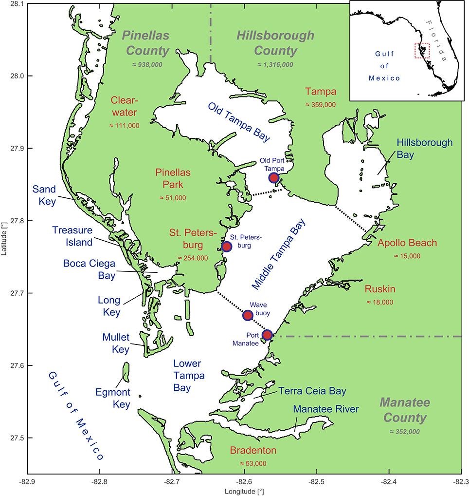
Figure 1. Map of Tampa Bay with its bay sections as well as adjacent cities and counties with 2014 population estimates (from United States Census Bureau); tide and wave gauges are marked as red dots.

The entire Tampa Bay has a surface of around 1033 km² (Kunneke and Palik, 1984) and is commonly divided into four major bay segments, also pictured in Figure 1. Old Tampa Bay and Hillsborough Bay are located in the north. Middle Tampa Bay forms the central region and Lower Tampa Bay connects with the Gulf of Mexico. Terra Ceia Bay and the tidal reach of the Manatee River are two segments in the south. Boca Ciega Bay creates the western coast of St. Petersburg and is protected by the islands Long Key, Treasure Island, and Sand Key. Egmont Key is located south of Mullet Key at the mouth of Tampa Bay, the connection between Lower Tampa Bay and the Gulf of Mexico. The alongshore profile of Egmont Key blocks more than a third of the Bay's mouth with a length of 3 km perpendicular to the outlet direction. Egmont Key arose from sediments provided by the Tampa Bay which were partially deposited in the ebb-tidal delta of the estuary due to the common action of tides and waves. The entire sediment complex below the barrier island extents 10 km into the Gulf of Mexico (Stott and Davis, 2003). The first detailed survey of Egmont Key dates back to 1877 and changes in shape and size were already documented at that time (see Figure 5 in Stott and Davis, 2003). Today the U.S. Army Corps of Engineers (USACE) tries to hinder the erosion of Egmont Key with beach nourishment measures which currently help maintaining the shape of the island.

Tampa Bay's connection to the Gulf of Mexico is narrowed by Egmont Key. A 30 m deep passage north of the island is used as the entrance to the main shipping channel. Overall Tampa Bay is characterized by shallow waters with an average depth of 3.5 m. Exceptions are, beside the mentioned outlet, the harbors and dredged shipping lanes to the ports of St. Petersburg, Tampa, and Port Manatee (Goodwin and Michaelis, 1984). The tidal regime is mixed semi-diurnal.

Like the entire Gulf region, the Tampa Bay area is threatened by tropical storms originating from the Atlantic Ocean or Caribbean Sea. In the past decades some severe tropical cyclones occurred in the eastern Gulf of Mexico but none directly passed through or close by the Tampa Bay area. The last direct hit of a major hurricane dates back to 1921 (Doehring et al., 1994; Weisberg and Zheng, 2006). Furthermore, strong winter storms and nor'easters also have the potential to cause storm surges in Tampa Bay with water levels comparable to those induced by tropical events (e.g., event in January 1987).

3. Methods

This study aims at investigating the effect of a barrier island loss on extreme still water levels and wind waves in the Tampa Bay. Therefore, we calibrate and validate a hydrodynamic numerical model, use control and scenario runs, and an extreme value analysis to quantify changes in extreme events. Results are presented as changes in return levels (of still water and significant wave height) due to the modeled barrier island loss.

3.1. Numerical Model Setup

The investigations are based on numerical model experiments requiring hydrodynamic forces at the open boundaries as input. The tides and waves within Tampa Bay are primarily from the Gulf of Mexico but there is no continuous water level hindcast available covering the period under investigation or the investigated area. This is why we set up a two-dimensional, depth-averaged, barotropic tide surge model covering the entire Gulf of Mexico, hereafter referred to as Gulf Model. This large-scale model is intended to provide water level boundary conditions for a higher resolution model of the main study area covering the entire Tampa Bay, hereafter referred to as Bay Model. This setup enables us to fully describe all relevant hydrodynamic processes adjacent to and within Tampa Bay. Detailed information and references for all data sets described below are summarized in Table 1. The numerical model setup is briefly summed up in Table 2.

TABLE 1

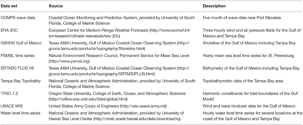
Table 1. Data sets and data sources used for the study.

TABLE 2

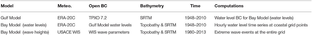
Table 2. Overview: set up numerical models, used input, boundary conditions (BC), and conducted computations.

The models are set up and computed using the open source modeling suite Delft3D, provided by Deltares (Lesser et al., 2004). The spatial discretization is achieved using curvilinear grids, shown in Figure 2. In the Gulf Model, cell sizes between 30 and 3 km are used. The grid resolution increases from west to east in order to provide the most accurate results in front of Tampa Bay without spending too much computation time. In the Bay Model, cell sizes range from 400 to 150 m, depending on location and grid curvature. Both models are configured within a coastline provided by the Gulf of Mexico Coastal Ocean Observing System (GCOOS) with a spatially consistent resolution of 60 m.

FIGURE 2

Figure 2. Curvilinear grids (blue) and shoreline (red) used for the Gulf Model (A) and for the Bay Model (B). For clearness, the grids in this figure appear with a coarser resolution than used for the simulation. The Gulf Model grid (A) is actually two times higher resolved, the Bay Model grid (B) three times higher. Black lines indicate the model boundaries of the Gulf Model in the Yucatán Channel (A1), in the Florida Strait (A2) as well as the boundary toward the Gulf of Mexico in the Bay Model (B1).

As bathymetric input, the SRTM30 PLUS V6 data set based on the Shuttle Radar Topography Mission (SRTM) is used. It covers the entire Gulf of Mexico including Tampa Bay on a 1′ grid which is equivalent to a grid cell size of approximately 1.85 km at Gulf-latitudes. Furthermore, the Tampa Bay “Topobathy” bathymetric dataset with a resolution of approximately 30 m on an equidistant grid provided by the National Oceanic and Atmospheric Administration (NOAA) is used to increase the accuracy of spatial information in the main area of interest. To estimate the impact that a loss of Egmont Key would have on Tampa Bay the bathymetry of the Bay Model is altered around today's location of the barrier island. The assumed disappearance is modeled by lowering the bathymetry of Egmont Key. The present day bathymetry is shown in Figure 3A. The new bed level is interpolated between today's depth around the island. Complete erosion is the worst-case scenario but plausible since Egmont Key is a sand accumulation and not sitting on a bed rock raise (Stott and Davis, 2003). The result from removing Egmont Key from the bathymetry is a wide, slightly inclined channel connecting the Gulf of Mexico with Tampa Bay (Figure 3B).

FIGURE 3

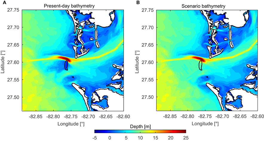
Figure 3. Unchanged control run bathymetry (A) and scenario bathymetry without Egmont Key (B).

The open boundaries of the Gulf Model are in the Florida Strait between the Everglades National Park (FL, USA) and Varadero (Cuba), and in the Yucatán Channel between Sandino (Cuba) and Cancún (Mexico) (see Figure 2A). Both boundaries are driven by astronomical tidal levels. As input we use phases and amplitudes of the main tidal constituents obtained from the global ocean tides model TPXO 7.2, provided by the College of Earth, Ocean, and Atmospheric Sciences at the Oregon State University. The Gulf Model is used to model the transition of the tidal components from the Atlantic into the Gulf of Mexico ocean basin. TPXO 7.2 contains 13 harmonic constituents (M2, S2, N2, K2, K1, O1, P1, Q1, MF, MM, M4, MS4, MN4) for each point on a global grid with a 0.25° resolution. Tidal boundary conditions are derived by interpolating the nearest TPXO 7.2 gridded information on the models open boundaries. Within both models, tidal forces acting on the entire body of water are also considered including eleven semi-diurnal, diurnal, and long period tidal constituents (M2, S2, N2, K2, K1, O1, P1, Q1, MF, MM, SSA). The water levels from the Gulf Model force the Bay Model at the boundary indicated in Figure 2B.

The models are additionally forced with spatially varying meteorological data (i.e., wind and atmospheric pressure fields) covering the entire model domain. We use data from the ERA-20C reanalysis provided by the European Centre for Medium-Range Weather Forecasts (ECMWF). The reanalysis data covers the period 1900–2010 and has a temporal resolution of 3 h and a spatial resolution of 1° on a global grid. For water level computations the years 1948–2010 have been chosen since observations at the gauge St. Petersburg (providing the longest record for the region) are limited to this period. The used reanalysis data are limited to the description of meteorological conditions at a supra-regional level due to the temporal and spatial resolution. Local and regional anomalies, e.g., in the proximity of tropical cyclones, are represented with little detail, but at the same time no major hurricane passed directly over Tampa Bay within the model time frame making the application of ERA-20C wind and pressure fields more suitable for the investigation area. The availability of the wave input from the USACE Wave Information Studies (WIS) project is restricted to the period 1980–2013. Therefore, wind data are also taken from this data base for the wave simulation as well as wave height, direction, amplitude, and spread information. The WIS hindcast is available at grid points along the entire U.S. coast. Three points close to the mouth of Tampa Bay are used to force the Bay Model. Between these points the boundary conditions are interpolated linearly.

In the Bay Model, mean sea level (MSL) changes are also considered using the Permanent Service for Mean Sea Level (PSMSL) time series of St. Petersburg obtained from the British Natural Environment Research Council. Since the computations for each year of the simulation time are run separately to handle the large output data, the MSL is adjusted according to the annual change in the PSMSL time series.

3.2. Numerical Model Calibration and Validation

The overall aim of this paper is to assess changes in both extreme still water levels along the coastline and wave heights as consequence of the loss of Egmont Key. Simplified, simulations of water level and wave height variables are conducted separately enabling to evaluate the contribution of each component to a total water level independently. Tides and wind set up off the mouth of Tampa Bay are extracted from three grid points of the Gulf Model. Bay Model water level time series are extracted at about 800 grid points along the coastline in intervals of approximately 1 km and wave parameters are extracted from the entire grid since we expect major changes off the coastline, with potential effects on navigation during extreme events.

In hydrological modeling various efficiency criteria are used to describe the goodness of model calibration (Krause et al., 2005). Here we use the coefficient of determination (r²) and the root mean squared error (RMSE). The coefficient of determination is defined as the squared value of the coefficient of correlation (Krause et al., 2005). The coefficient is calculated with observed (x_o) and simulated (x_s) water level time series, each with k corresponding values:

$\begin{array}{ll}{r}^2={\left[\frac{{\displaystyle {\sum }_{i=1}^k}\left(x_{si}-{\overline{x}}_s\right)\left(x_{oi}-{\overline{x}}_o\right)}{\sqrt{{\displaystyle {\sum }_{i=1}^k}{\left(x_{oi}-{\overline{x}}_o\right)}^2}\sqrt{{\displaystyle {\sum }_{i=1}^k}{\left(x_{si}-{\overline{x}}_s\right)}^2}}\right]}^2& (1)\end{array}$

A value of r² = 1 [-] denotes that both time series, observed and simulated, are identical. A value of r² = 0 [-] indicates that there is no correlation (Krause et al., 2005). The root mean squared error is calculated using the time series mentioned above with k values:

$\begin{array}{ll}\mathrm{\text{RMSE}}=\sqrt{\frac{1}{k}{\displaystyle \sum _{i=1}^k}{\left(x_{oi}-x_{si}\right)}^2}& (2)\end{array}$

The calibration of the models is done stepwise by adjusting the modeled water levels to recorded data at specific locations using the introduced efficiency criteria. The Gulf Model is calibrated first since this model provides the input of the Bay Model. The tide gauge of Clearwater, located approximately 45 km north of the mouth of Tampa Bay is used as reference for the calibration. Furthermore, three tide gauges at the U.S. Gulf coast are used to check the model performance including Apalachicola (Florida), Grand Isle (Louisiana), and Galveston Pier (Texas). All time series are obtained from the NOAA tide gauge data base.

The Gulf Model's parameters and boundary conditions are adjusted in two steps. In the first step a calibration is done by varying the Manning's roughness coefficients (n values). In the second step the harmonic constituents at the open boundaries of the Gulf Model are adjusted. At the beginning of the calibration exercise, the n values are very uncertain. The Gulf Model is calibrated by iteratively computing the model with varying Manning's n values in the range 0.02 ≤ n ≤ 0.04 s/m^1/3 and comparing the computation results (using the test statistics described above) with the tidal predictions from the tide gauge Clearwater provided by NOAA. The calibration consists of multiple simulations over 1 month periods, in each case with a spin-up time of 2 weeks.

A Manning's roughness of n = 0.035 s/m^1/3 shows the smallest achievable error with unmodified harmonic constituents. Using this roughness significantly increases the accuracy of the model results but deviations of up to 10 cm are still present. To reduce the remaining differences between simulated and observed data the second calibration step is conducted. The input of amplitudes and phases for each boundary point at the Florida Strait and the Yucatán Channel is corrected by adjusting the input amplitudes and phases in order to minimize the error. Similar to the roughness calibration this is done iteratively.

Tidal predictions provided by NOAA are separated into their underlying constituents and individually compared to the corresponding constituents from the simulation results. The tidal analyses are performed with the T_TIDE tool by Pawlowicz et al. (2002). The component breakdown shows which tidal components have the largest influence on the errors. Errors are reduced by the adjustment of corresponding constituents (amplitudes and phases) at the boundaries. A linear dependence between constituents at the gauge site and at the boundaries is assumed for the iterative calibration process. This approach disregards that tidal oscillations at the gauge are a combination of tidal oscillations at the boundaries and tides originating from the Gulf of Mexico but yet leads to a fast convergence of observed and simulated constituents. After calibration the correction factors for the amplitude f_amp are in a range of 0.9 ≤ f_amp ≤ 1.4 [-] and the addends for the phase f_pha in the range of −60° ≤ f_pha ≤ 15° respectively. All correction factors and addends are presented in Table 3.

TABLE 3

Table 3. Factors f_amp and addends f_pha used to correct the Gulf Model input amplitudes and phases.

After calibration the comparison of full time series at gauge Clearwater results in a coefficient of determination of r² = 0.96 [-], showing that the model reliably reproduces observed water levels at this site, close to the mouth of Tampa Bay. The RMSE calculation shows errors of 5.1 cm for tidal high water levels and 5.7 cm for tidal low water levels. The observed mean tidal range at gauge Clearwater is 58 cm. Overall the model tends to overestimate the minor high and low waters of the mixed semi-diurnal tide cycle, whereas higher high waters are computed more reliably enabling to simulate extremes properly.

The Bay Model is forced with the Gulf Model water levels and also calibrated. The calibration of the Bay Model is limited to the adjustment of the Manning's roughness coefficient n. The input boundary condition has been computed by the calibrated Gulf Model and therefore should not be changed. Tampa Bay is monitored by several hydrological and meteorological measuring stations. Three of four active tide gauges within the estuary are unaffected by inflowing rivers and are used here for calibration, validation, and bias correction of the Bay Model. These stations are located at the port of St. Petersburg in the west of the bay, at Port Manatee in the south-east, and at Old Port Tampa in the north (see Figure 1). The official tide predictions for these gauges, provided by NOAA, are used as reference. The roughness calibration is conducted in the same way the Gulf Model has been calibrated. The iterative test considers values in the range of 0.02 ≤ n ≤ 0.036 s/m^1/3. The best fit of simulated time series against observed time series, regarding RMSE and coefficient of determination, is achieved by using a Manning's roughness coefficient of n = 0.022 s/m^1/3. The smaller coefficient, compared to the Gulf Model's roughness, is attributable to the significantly higher resolution of the seafloor topography in the Bay. The rather coarse resolution of the Gulf bathymetry only allows a smoothed seafloor in the Gulf Model. Geometric features smaller than the bathymetry resolution have to be added artificially by increasing the roughness. The Bay Model's bathymetry already depicts most of these features. Therefore, the calibration leads to a smaller roughness coefficient. The efficiency criteria after Krause et al. (2005) described above are also calculated for the Bay Model calibration results. RMSE and r² differ from gauge to gauge within Tampa Bay. Regarding tidal high water levels the RMSE does not exceed 4 cm; the coefficient of determination spans 0.92 ≤ r² ≤ 0.95 [-]. The comparison of full time series also shows an RMSE of approximately 4 cm and r² ≥ 0.95 [-] for all three gauges.

The wave simulations are conducted using the calibrated water level model of the Bay. A validation run (focusing on the significant wave height) has been performed indicating that the model reproduces large wave events well for the simulated period using one available buoy data set of the Coastal Ocean Monitoring and Prediction System (COMPS). The buoy data was recorded at the border of Middle and Lower Tampa Bay (see Figure 1) covering 5 months (April through August 2012) with hourly wave parameters. Several events from this period have been simulated. The model tends to underestimate small wave heights. With focus on the three largest events a comparison between simulated and observed significant wave heights gives an RMSE of 12 cm and r² = 0.83 [-] where absolute values range from 86 to 91 cm. The largest event shows a deviation of 3 cm in significant wave height. Based on the USACE WIS data only events larger than the tested wave heights are simulated for the comparison between control and scenario run. Therefore, the model can be used for the simulations disregarding the deficiencies in estimating small wave heights. Regarding wave periods the model shows peak periods of approximately 3 s for the highest events at the location of the wave buoy. Due to large gaps in the wave period record a validation of this parameter could not be conducted.

3.3. Statistical model setup

3.3.1. Pre-processing

The numerical model is used to simulate multi-decadal water level and wind wave time series which are required for reliable extreme value analysis (EVA) of both variables. Extreme water levels are assessed at individual grid points along the entire Tampa Bay coastline. The wave simulations are used to estimate return wave heights for the entire grid. In both cases, simulations are performed using (A) a current state bathymetry (control run) and (B) a bathymetry where Egmont Key is removed (scenario run; see Figure 3). Both water level simulations consider the same time period of 63 years (1948–2010) and the same hydrodynamic and meteorological boundary conditions. The wave simulations are only conducted for extreme events, since a continuous simulation of several consecutive years would be computationally much more expensive without adding new relevant information on extremes. Furthermore, the available wave data used as input at the open boundaries is event based (not continuous) and covers the period 1980–2013. The results from the different model runs are used for the EVA.

A fundamental assumption for EVA is that time series are stationary and that events are independent (Coles, 2001; Arns et al., 2013). This is why linear detrending has been applied to all time series (simulated and observed) in order to account for the first criterion. To comply with the second criterion a declustering procedure has been applied to the data ensuring that the sample consists of independent events. The declustering procedure is conducted as follows: at first all peaks within the simulated and detrended hourly water level time series are selected and matched with the corresponding peaks in the detrended observation time series. Clusters are detected by identifying peaks that occurred within 6 h. A simple comparison of two neighboring peaks that fulfill the 6-h-criterion allows discarding the smaller one since this peak is assumed to be not independent of the larger one. Finally, only the largest peak of a tidal high water period is used for the EVA (Zachary et al., 1998).

3.3.2. Bias Correction

The model calibration successfully reduced the error between simulated and observed water levels but significant differences still remained due to model imperfections. This bias can be visualized by plotting observed water levels against the corresponding simulated water levels, as shown in Figure 4A. The regression (red) indicates the best linear fit against the scatter diagram in a least squares sense using the orthogonal distance of each point from the fit (orthogonal fit). The bias is the difference between the regression and the angle bisector (black, target regression), expressed as location and slope deviation. A parametric bias correction of the extreme water levels, as described in the following, has been conducted prior to the EVA in order to eliminate these deviations.

FIGURE 4

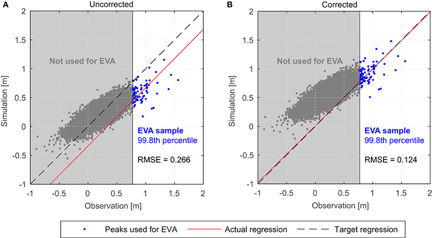
Figure 4. Uncorrected water levels (A) and corrected water levels after the parametric bias correction (B).

In case of a parametric bias correction the difference function between orthogonal fit and angle bisector is used to adjust the simulated values. A non-parametric or empirical bias correction adjusts each simulation value based on the absolute deviation from the observed value (Mudelsee et al., 2010). The empirical approach results in exactly corrected simulation values while the parametric correction shifts the values according to the correction function but does not eliminate the spreading. An advantage of the parametric approach, however, is that the correction function describes a systematic model error, e.g., a model tending to generally simulate too high or too low water levels as shown in Figure 4A. Therefore, the function determined for a site can be used to correct the same systematic error at all other locations even if the absolute values differ between the sites. Furthermore, the parametric approach can be used to adjust scenario data where systematic model errors are assumed to be consistent throughout all model runs.

In this study, the correction is applied to the largest Tampa Bay model results using observational data from St. Petersburg tide gauge covering the entire simulation period (1948–2010). We focus on the 99.8th percentile of threshold exceedances since only these data are used in the following EVA. Observations from the tide gauges at Port Manatee and Old Port Tampa are additionally used between 1999 and 2010. Simulated peaks in Tampa Bay are adjusted according to the differences between target data and orthogonal regression fit at each individual tide gauge. Results of this correction are shown exemplarily in Figure 4B. Following this procedure, data sets at all ungauged grid points of the Bay Model are corrected using the correction factors estimated at the gauged sites. For the years 1999–2010, in which factors for all three gauges are available, an inverse distance weighting approach is used to interpolate the factors to ungauged locations along the entire Tampa Bay coastline. It is assumed that the bias mainly originates from model limitations, like the discretization of wind data or seafloor topography approximations. Therefore, the correction is also applied to the scenario run. Corrected scenario water levels are obtained by calculating the differences between uncorrected control and scenario run water levels and then adding them to the corrected control run water levels.

The wave control run has not been adjusted as the available wave data required as input for developing a bias correction only covers 5 months with only one extreme event on record. Thus, a reliable correction cannot be derived. In our numerical sensitivity study, we focus on changes in wave heights as consequence of a potential loss of Egmont Key. The overall aim of this assessment is to estimate relative changes in wave heights. Based on our validation we assume that the model is able to capture these changes reliably.

3.3.3. Return Level Assessment

The return level assessment is conducted with both control run and scenario run water level data at individual grid points along the Tampa Bay coastline and with the corresponding wave simulations with the intention to estimate the impact of the disappearing of Egmont Key. Two extreme value analysis approaches are tested prior to the final assessment, i.e., the Bock Maxima (BM) method using the Generalized Extreme Value Distribution (GEV) and the Peak-over-threshold (POT) method with the Generalized Pareto Distribution (GPD).

The BM sampling approach considers the r largest events within a specific time frame, e.g., the three highest water levels of each year. This yields a sample of events which allows an estimation of return water levels by fitting the GEV to the sample. The GEV unifies three fundamental extreme value distributions namely the Gumbel, Fréchet, and Weibull and is defined in Equation 3 with the location parameter −∞ < μ < ∞, the scale parameter σ > 0, the shape parameter −∞ < ξ < ∞, and the BM values z (Coles, 2001):

$\begin{array}{ll}GEV=exp\left\{-{\left[1+\xi \left(\frac{z-\mu }{\sigma }\right)\right]}^{-1∕\xi }\right\}& (3)\end{array}$

The POT sampling approach considers all values that exceed a defined threshold u, e.g., the 0.5% largest values of a record also referred to as the 99.5th percentile. The GPD is related to this sampling method and also couples various extreme value distributions. It is defined as

$\begin{array}{ll}GPD=1-{\left(1+\frac{\xi ·z}{\sigma +\xi ·\left(u-\mu \right)}\right)}^{-1∕\xi }& (4)\end{array}$

where μ, σ, ξ, and z denote parameters and values as above (Coles, 2001).

The BM method has been tested with r ∈ {1, 2, 3} values per year and the POT approach with the 99.6, 99.7, and 99.8th percentile of threshold exceedances. Both methods have been applied to subsets of observed and simulated time series of the tide gauge of St. Petersburg. The 100-year return water level has been estimated with both methods and different extreme value model setups using varying time series lengths. The results are shown in Figure 5 indicating that the POT approach with the 99.8th percentile yields the most robust results. Compared to other approaches, these estimates are among the smallest variances of all return levels considering different time series lengths (within a range of 10 cm). The gray shade in Figure 5 denotes time series lengths that are too short for a reliable 100-year return level estimation. Therefore, the results within and close to the shade vary heavily. With longer time series (especially starting between 1948 and 1964) the results are more robust, even when very large events (often associated with tropical cyclones) are excluded from the return level assessment (e.g., Hurricane Easy, 1950). Furthermore, this method with the 99.8th percentile subset only causes small differences of approximately 10 cm between return levels estimated from the observed and from the simulated time series using the longest period available. Other EVA model setups yield differences of up to 40 cm. Remaining small deviations are assumed to be negligible as we aim at investigating the changes induced by the vanishing of Egmont Key and deviations are caused by consistent model deficiencies that affect control and scenario runs alike.

FIGURE 5

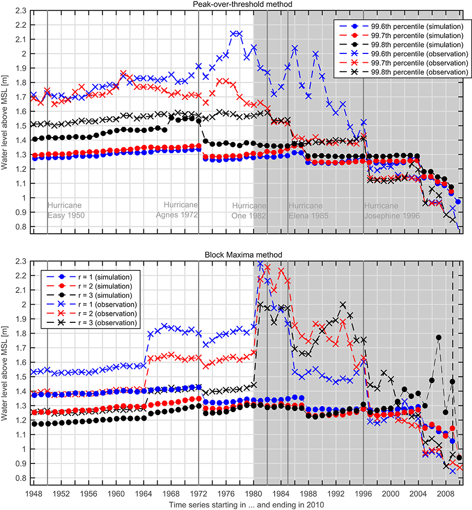
Figure 5. Testing statistical approaches: 100-year return water level, estimated with different samples (colors) and with decreasing time series lengths (x-axis); the gray background denotes time series lengths which are too short for a reliable return level estimation (<30 years).

Frequencies and magnitudes of extreme wave heights are estimated using the same approach as described above. However, in that case we use the 99.5th percentile of all events of the USACE WIS database. These selected extreme events are simulated individually using the control run and scenario bathymetries.

4. Results

4.1. Return Water Levels

Extreme water levels are assessed for different return periods including the 5-, 25-, 50-, 100-, and 200-year events. Thus, the return period estimation does not exceed 3 to 4 times the length of the underlying time series. The latter limit is recommended e.g., by Pugh (2004). The differences in return water levels are visualized in Figures 6, 7 for the 25- and 100-year events, respectively. The return water levels are only used for estimating the differences a loss of Egmont Key would cause.

FIGURE 6

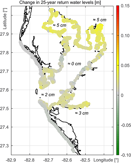
Figure 6. Change in 25-year return water levels for available grid points along the Tampa Bay and Gulf coastline.

FIGURE 7

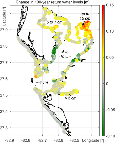
Figure 7. Change in 100-year return water levels for available grid points along the Tampa Bay and Gulf coastline.

A comparison of Figures 6, 7 indicates the overall development of the results. Changes in water levels with return periods shorter than 100 years appear to have a spatially different characteristic compared to those with return periods greater than or equal to 100 years. At shorter return periods, increases can be found along the entire Tampa Bay coastline with significant changes in Hillsborough Bay and Old Tampa Bay. For a return period of 25 years, increases between 3 and 5 cm are found. At the tidal reach of the Manatee River and the coastline of Lower Tampa Bay, close to the mouth of the estuary, increases are in the order of 2 to 3 cm. Middle Tampa Bay is not affected. Regarding return periods of 100 years or more, largest return water level increases are found along Hillsborough Bay. Water levels increase by up to 15 cm. There are also changes in Old Tampa Bay reaching 5 to 7 cm. The coastlines along the Manatee River and at Lower Tampa Bay would undergo changes in the 100-year event of only a few centimeters if Egmont Key disappeared. Parts of Middle Tampa Bay would even experience a small decrease. The development of extreme water levels in the Tampa Bay in case of a loss of Egmont Key is affirmed regarding the change in the 200-year return water levels (not shown). In Hillsborough Bay the return water levels would increase up to 30 cm whereas at the coast of Middle Tampa Bay they would decrease up to 20 cm.

The return level assessment reveals that Egmont Key has a significant reducing influence on extreme water levels in the Tampa Bay. The northern parts of the estuary are protected by the barrier island and would be affected negatively by a loss of the barrier island. Even the smaller but more frequent storm surge events would increase along large parts of the Tampa Bay coastline.

In addition to the EVA results, differences in maximum water levels (scenario to control run) along the coast as well as relative increases have been calculated (Figures 8A,B). A loss of Egmont Key leads to water level increases of more than 4 cm in the entire Tampa Bay. Manatee River, Lower Tampa Bay, and northern Hillsborough Bay water levels increase up to 12 cm which is a change of up to 10%.

FIGURE 8

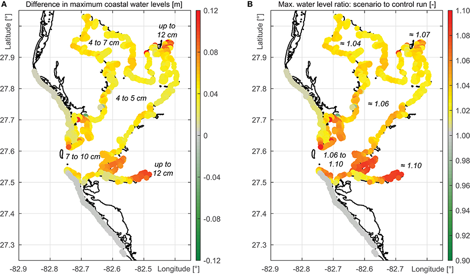
Figure 8. Difference in maximum water levels along the coastline (A) and the difference expressed as ratio between scenario and control run simulation (B).

4.2. Return Wave Heights

Extreme wave heights are estimated at each grid point including areas of particular interest like shipping lanes and coastal zones. Overall the wave heights show strong increases around the location of today's Egmont Key in the Gulf of Mexico as well as in Lower Tampa Bay. The estimated wave heights for a return period of 25 years are shown in Figure 9. Entire Lower Tampa Bay would be affected with increases of mostly 0.4 to 1.0 m in areas without bathymetric changes. Close to today's location of Egmont Key, where the bathymetry has been changed, increases range from 1.3 to 1.7 m. In contrast, Middle Tampa Bay only shows increases of a few centimeters along the center line of the estuary and the northern parts of Tampa Bay are not affected at all.

FIGURE 9

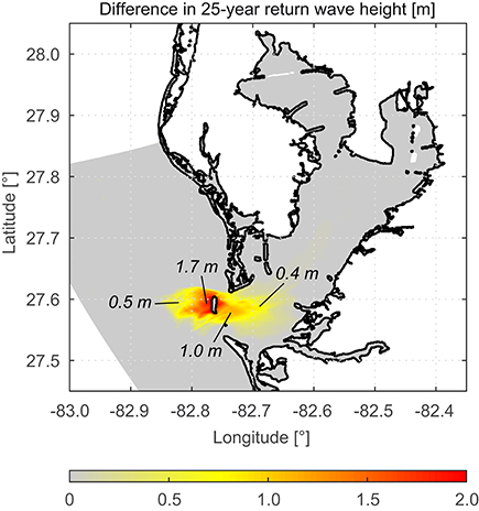
Figure 9. Change in 25-year return wave height for all grid points.

Besides the EVA results, the maximum differences between the control and the scenario run and also the relative increases of wave heights have been calculated for each grid point (see Figures 10A,B respectively). Both plots confirm that changes in wave heights are only found in the Lower Tampa Bay area. Maximum differences between 1.5 and 2.0 m around the location of the barrier island could have a significant impact on the navigability since these increases are a doubling of the today's wave heights in this area. The eastern coast of Lower Tampa Bay would also see significant increases in wave heights (up to 300%). For the city Anna Maria, located on the barrier island south of Egmont Key, wave height increases of up to 13 cm are found.

FIGURE 10

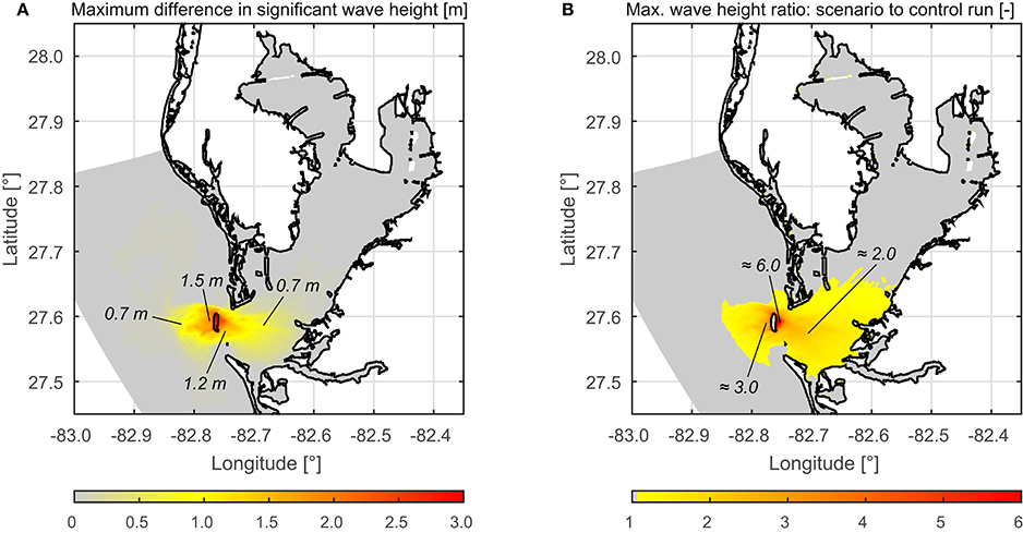
Figure 10. Maximum difference in significant wave height considering all simulated events (A) and the difference expressed as ratio between scenario and control run simulation (B).

Regarding the change in wave period increases are limited to the area described above. The loss of sheltering and the increased depth directly behind today's location of Egmont Key result in periods of 9 to 12 s in Lower Tampa Bay under scenario conditions where control runs show periods of 3 to 5 s. Wave directions are affected by the removal of Egmont Key as well, but only in close vicinity to the barrier island.

5. Discussion and Conclusions

The simulation of water levels and waves in the Tampa Bay with and without the barrier island Egmont Key shows that the island provides significant natural coastal protection. For extreme still water levels the removal of Egmont Key from the model's bathymetry yielded higher return water levels in the northern parts of the estuary. The absence of the barrier that blocks about a third of the mouth of Tampa Bay allows westerly winds to generate more wind set-up in the estuary. The northern bay sections as well as the Manatee River are affected most due to the very shallow waters and narrow connections to Middle Tampa Bay that only allow a limited near-ground back flow. The extreme water level increases in the northern bay sections are expected to be larger than a decimeter in case of a 100-year event which is a change of about 10%. The affected areas are densely populated and developed with residential, commercial, and industrial infrastructure close to the waterfront. Smaller events that occur more frequently (e.g., 25-year return period) are also expected to increase when Egmont Key disappears. From a coastal protection perspective, it is thus reasonable to put effort in the maintenance of Egmont Key since large parts of the adjacent mainland is low-lying and therefore already vulnerable to extreme water levels and waves. An increase in extreme events, adding up on the existing level, would increase the ecological and economical risk.

Middle Tampa Bay shows only small increases in 25-year return levels and even a decrease in the 100-year water level. This can primarily be attributed to a change of the shape parameter of the extreme value distribution. In this area, under scenario conditions, relative increases of smaller events are larger than those of the most extreme events. Therefore, the EVA leads to smaller return levels, especially for longer return periods. We speculate that the most extreme events do not increase as much as the smaller events due to an increased back flow since the removal of the barrier island also enlarges the outflow cross-section.

The wave height assessment shows that the potential loss of Egmont Key has a significant impact on the waves in Lower Tampa Bay but overall the influence occurs locally. The effect of Egmont Key is limited to an area which extends approximately 10 km into the Bay, measured from today's location of the island. Increasing wave heights in this area can be attributed to the missing barrier which today shelters Lower Tampa Bay directly, and to the increased depth around the location of Egmont Key. Areas in the northern Tampa Bay are protected by the shallow waters of the estuary, which would dissipate most wave energy in case that Egmont Key completely disappears. The very local change in wave directions is also attributable to the increased depth. With the loss of Egmont Key and the increase in water depth local shallow water effects like refraction and diffraction do not appear anymore. Waves from the Gulf of Mexico enter Tampa Bay unchanged until the depth limitation decreases wave heights significantly.

The EVA has been conducted without distinguishing between event types. Tampa Bay is located in an area where tropical cyclones occur during summer and fall months. Therefore, separate analyses of tropical and extra-tropical events would be a reasonable approach, as described e.g., by Haigh et al. (2014). Furthermore, this would be necessary in case that the study aims at estimating absolute heights for return periods. The simplified method used in this study is feasible since no major tropical cyclone directly hit Tampa Bay within the time period of interest. Figure 11 shows that tropical and extra-tropical events in Tampa Bay led to similar total still water levels. Possible changes from other extreme events that occured beyond the period of observation are not considered in this particular study but could also have an effect on the shape of the underlying extreme value distribution. Additionally the return levels are only used for the A-B-comparison and therefore the chosen simplified method leads to suitable results.

FIGURE 11

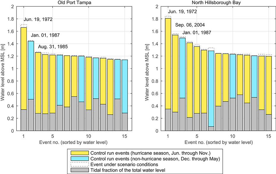
Figure 11. Comparison of the 15 largest events (by total still water level under control run conditions) in northern Tampa Bay. Yellow bars indicate storm surges during the tropical season (June through November), blue bars indicate all other events (e.g., winter storms). The tidal contribution to the water level is depicted as gray overlay. The total water level under scenario conditions is shown as dotted bar edges.

Figure 11 also shows the tide-surge-ratio of the top events in Tampa Bay. Haigh et al. (2010) detected an underestimation for large return periods when using direct methods (i.e., conducting an EVA with the total water level signal instead of modeling and examining tide and surge components separately) in case that the tidal component is larger than twice the size of the non-tidal component. In this context, the large contribution of the surge component to the total still water levels in Tampa Bay confirms the applicability of the direct approach.

Regarding the analyzed processes, this study focuses on water levels and waves. Changes in estuarine circulations have been neglected but may also be significantly affected by a loss of Egmont Key. In particular, changes in the tidal prism, tidal currents, exchange circulation and flushing could occur. These changes are associated with alterations in the entire ecosystem and should be investigated in further studies.

Overall the complete removal of Egmont Key is a simplified approach and disregards other morphologic changes in the barrier island system which would probably occur simultaneously with an erosion of the island extending over several decades. Examples are coastline changes in Tampa Bay or at the Gulf coast near the mouth of the estuary, changes in depth due to sediment displacement, and the impact of sea level rise. Albeit using a worst-case scenario, the presented results show that Egmont Key significantly alters extreme events in Tampa Bay and that a detailed investigation of realistic scenarios is needed. Further studies could include the above-mentioned morphologic and hydrodynamic changes to improve the results. Furthermore, inundation of the low-lying islands and of the mainland during storm surges should be considered. Authorities and coastal managers could benefit from the results and use the findings to develop appropriate protection strategies for the Tampa Bay area.

Author Contributions

AA, TW, and MU developed the concept. MU set up and ran the models, analyzed output data, and drafted the paper with the guidance of AA. SM provided fundamental model data. All authors revised and finalized the draft. ML and JJ supervised the research project and finally approved the paper.

Conflict of Interest Statement

The authors declare that the research was conducted in the absence of any commercial or financial relationships that could be construed as a potential conflict of interest.

Acknowledgments

All analyses presented in this paper were part of the project The effect of eroding barrier islands on coastal flood risk and estuarine health (project ID 57052194), supported by the German Academic Exchange Service (DAAD) with funds of the German Federal Ministry of Education and Research (BMBF).

References

Arns, A., Wahl, T., Haigh, I. D., Jensen, J., and Pattiaratchi, C. (2013). Estimating extreme water level probabilities: a comparison of the direct methods and recommendations for best practise. Coast. Eng. 81, 51–66. doi: 10.1016/j.coastaleng.2013.07.003

CrossRef Full Text | Google Scholar

Coles, S. (2001). An Introduction to Statistical Modeling of Extreme Values. London: Springer.

Google Scholar

Cromwell, J. E. (1973). “Barrier coast distribution: a world survey,” in Barrier Islands. Benchmark Papers in Geology, Vol. 9, ed M. L. Schwartz, (Stroudsburg, PA: Douden, Hutchinson, and Ross), 407–408.

Doehring, F., Duedall, I. W., and Williams, J. M. (1994). Florida Hurricanes and Tropical Storms: 1871-1993: An Historical Survey, Vol. 71 of Technical Paper. Gainesville, FL: Florida Sea Grant College Program, University of Florida.

Goodwin, C. R., and Michaelis, D. M. (1984). Appearance and Water Quality of Turbidity Plumes Produced by Dredging in Tampa Bay, Florida, Vol. 2192 of United States Geological Survey Water-Supply Paper. Washington: G.P.O.

Haigh, I. D., MacPherson, L. R., Mason, M. S., Wijeratne, E. M. S., Pattiaratchi, C. B., Crompton, R. P., et al. (2014). Estimating present day extreme water level exceedance probabilities around the coastline of australia: tropical cyclone-induced storm surges. Clim. Dyn. 42, 139–157. doi: 10.1007/s00382-012-1653-0

CrossRef Full Text | Google Scholar

Haigh, I. D., Nicholls, R., and Wells, N. (2010). A comparison of the main methods for estimating probabilities of extreme still water levels. Coast. Eng. 57, 838–849. doi: 10.1016/j.coastaleng.2010.04.002

CrossRef Full Text | Google Scholar

Krause, P., Boyle, D. P., and Bäse, F. (2005). Comparison of different efficiency criteria for hydrological model assessment. Adv. Geosci. 5, 89–97. doi: 10.5194/adgeo-5-89-2005

CrossRef Full Text | Google Scholar

Kunneke, J. T., and Palik, T. F. (1984). Tampa Bay Environmental Atlas, Vol. 85 (15) of Biological Report / Fish and Wildlife Service. Washington, DC: Fish and Wildlife Service, U.S. Dept. of the Interior.

Lesser, G. R., Roelvink, J. A., van Kester, J. A. T. M., and Stelling, G. S. (2004). Development and validation of a three-dimensional morphological model. Coast. Eng. 51, 883–915. doi: 10.1016/j.coastaleng.2004.07.014

CrossRef Full Text | Google Scholar

List, J. H., and Hansen, M. E. (1992). “The value of barrier islands: 1. Mitigation of locally-generated wind-wave attack on the mainland,” in Open-File Report (St. Petersburg, FL: United States Geological Survey), 92–722.

Mudelsee, M., Chirila, D., Deutschländer, T., Döring, C., Haerter, J., Hagemann, S., et al. (2010). Climate Model Bias Correction und die Deutsche Anpassungsstrategie. DMG Mitteilungen 03/2010, 2–7. doi: 10.013/epic.37089

CrossRef Full Text | Google Scholar

Oertel, G. F. (1985). The barrier island system. Marine Geol. 63, 1–18. doi: 10.1016/0025-3227(85)90077-5

CrossRef Full Text | Google Scholar

Passeri, D. L., Hagen, S. C., Bilskie, M. V., and Medeiros, S. C. (2015a). On the significance of incorporating shoreline changes for evaluating coastal hydrodynamics under sea level rise scenarios. Nat. Hazards 75, 1599–1617. doi: 10.1007/s11069-014-1386-y

CrossRef Full Text | Google Scholar

Passeri, D. L., Hagen, S. C., Medeiros, S. C., and Bilskie, M. V. (2015b). Impacts of historic morphology and sea level rise on tidal hydrodynamics in a microtidal estuary (Grand Bay, Mississippi). Continent. Shelf Res. 111, 150–158. doi: 10.1016/j.csr.2015.08.001

CrossRef Full Text | Google Scholar

Pawlowicz, R., Beardsley, B., and Lentz, S. (2002). Classical tidal harmonic analysis including error estimates in MATLAB using T_TIDE. Comput. Geosci. 28, 929–937. doi: 10.1016/S0098-3004(02)00013-4

CrossRef Full Text | Google Scholar

Pugh, D. (2004). Changing Sea Levels: Effects of Tides, Weather and Climate. Cambridge: Cambridge University Press.

Google Scholar

Stone, G. W., and McBride, R. A. (1998). Louisiana barrier islands and their importance in wetland protection: forecasting shoreline change and subsequent response of wave climate. J. Coast. Res. 14, 900–915.

Google Scholar

Stone, G. W., Zhang, X., and Sheremet, A. (2005). The role of Barrier Islands, muddy shelf and reefs in mitigating the wave field along coastal Louisiana. J. Coast. Res. 44, 40–55. Available online at: http://www.jstor.org/stable/25737048

Stott, J. K., and Davis, R. A. (2003). Geologic development and morphodynamics of Egmont Key, Florida. Marine Geol. 200, 61–76. doi: 10.1016/S0025-3227(03)00177-4

CrossRef Full Text | Google Scholar

Stutz, M. L., and Pilkey, O. H. (2001). A review of global barrier island distribution. J. Coast. Res. 34, 15–22. Available online at: http://www.jstor.org/stable/25736270

Weisberg, R. H., and Zheng, L. (2006). Hurricane storm surge simulations for Tampa Bay. Estuar. Coast 29, 899–913. doi: 10.1007/BF02798649

CrossRef Full Text | Google Scholar

Zachary, S., Feld, G., Ward, G., and Wolfram, J. (1998). Multivariate extrapolation in the offshore environment. Appl. Ocean Res. 20, 273–295. doi: 10.1016/S0141-1187(98)00027-3

CrossRef Full Text | Google Scholar