RecoMIA—Recommendations for Marine Image Annotation: Lessons Learned and Future Directions

1. Introduction

Optical imaging has a long tradition in marine sciences regarding its application to capture and visualize features of underwater environments such as fauna, flora, geological structures, litter, or infrastructure (Kocak and Caimi, 2005). Due to the technological advances and the increasing necessity to explore, map, and monitor the marine environment for anthropogenic impacts and new resources on a larger spatial scale, marine imaging applications have changed regarding scale and function. A variety of underwater observation platforms, such as Remotely Operating Vehicles, Baited Remote Underwater Video Systems, Autonomous Underwater Vehicles, Ocean Floor Observation Systems, Fixed long term Underwater Observatories are equipped with high resolution cameras to collect Gigabytes to Terabytes of image data, ranging from still images, over video recordings to high-dimensional hyper-spectral image data. Optical imaging represents a bridge technology between hydro-acoustic data (low spatial resolution and large scale mapping) and physical data (e.g., BoxCorer, MultiCorer - high spatial resolution and low sampling rate). As a consequence, large image and video collections are nowadays accumulated during cruises. The content of the images needs to be extracted and integrated with other data to be considered in scientific analysis or integrated in decision making processes. This extraction step is the non-trivial procedure of mapping images/video frames to nominal, qualitative, or quantitative data and is the main challenge in image analysis. Following to this extraction the image/video content can be represented in tables or spreadsheets. That way it can be subject to a statistical analysis and related to other dimensions such as time, space, or other sensor data. But the sheer volume of the image data, the high costs for the manual data extraction by trained human observers (e.g., marine biologists), the limited availability of expert taxonomists results in a serious bottleneck. This bottleneck in underwater image analysis gets more serious due to the continuous increase in spatial and temporal resolution. Just 10 years ago, benthic images of the sea floor showed a visual footprint of ~ 3 m² and nowadays visual footprints of more than 400 m² can be recorded. Hence an observer has to spend more time to visually explore the whole image. The marine image analysis community faces the fact that the traditional approach with one observer, manually viewing and annotating all the image data collected in one session is not applicable any more in a growing number of projects.

To solve the bottleneck problem, computational support is needed. Actions have been taken very early to support long-term data safety and storage, leaving the semantic annotation issue more or less untouched. This has changed in the last 5–10 years and marine image analysis has been identified as a new field of research for application-oriented computer science. The entire field could be referred to as marine image informatics, and includes concepts of database engineering, data mining, signal/image processing, pattern recognition, and machine learning. Marine image informatics is thus similar to bioinformatics/computational biology.

One distinct branch in marine image informatics research is the development of tools to support the manual data extraction process in marine images with new image annotation software tools. These tools improve the availability of data and streamline the data extraction process. To increase the data throughput and the annotation quality data sharing and collaboration via the web is supported by some of these tools. This is motivated by two trends. First, research in the natural sciences is carried out more and more in interdisciplinary collaborations to address the multi-dimensional aspects of scientific questions (Lakhani et al., 2006; Wuchty et al., 2007; Shneiderman, 2008; Rylance, 2015). Second, nowadays web technology allows interdisciplinary collaboration between different groups on a new level regarding the sharing of data and knowledge which is sometimes referred to as Science 2.0 (Waldrop, 2008).

Some of the proposed marine image annotation tools like NICAMS (NIWA Image Capture and Management System)¹, VARS (Video Annotation and Reference System)², and VIDLIB (Marcon et al., 2015) are desktop applications and support the observers in marking regions or points in images and linking those to semantic/taxonomic categories. Another very popular example is the Coral Point Count software, that is frequently used to assess the abundance of different corals in images by manual classification of random point seeds (Kohler and Gill, 2006). Other and more recent approaches [e.g., CATAMI (Collaborative and Automated Tools for Analysis of Marine Imagery)³, SQUIDLE⁴, CoralNet (Beijbom et al., 2015), or BIIGLE (BioImage Indexing, Graphical Labeling and Exploration) (Ontrup et al., 2009; Schoening et al., 2009)], are web-based systems, making use of today's broad internet bandwidth and software technology to address Science 2.0 driven specifications. In summary, marine scientists now are equipped with different software and web tools to support saving, managing, exploring, sharing image data, and annotating marine imagery. Usually, the tools are used by human expert observers to extract nominal, qualitative, or quantitative data from the images. The observers inspect the image/video data on a screen, visually detect objects of interest (OOI, e.g., biota) or regions of interest (ROI, e.g., resource occurrences, coral structures, or bacterial mats) and (in many cases) mark the position (i.e., a set of pixels) of those objects/regions with an input device (e.g., a computer mouse or a draw pad). Finally, a semantic category has to be assigned to the OOI/ROI. In some cases, the spatial level of detail in the data extraction process is rather low, so entire images are assigned to semantic categories, e.g., the dominant substrate type.

For the sake of compactness we will omit the term OOI and concentrate on ROI without any restriction. Additionally, we will omit the term “video” in the following. Please note that the observations, guidelines and considerations in the paper can be applied to video annotation in a straightforward way if the video is analyzed as a series of extracted video frames that can be interpreted the same way as still images [as it was done for instance in Purser et al. (2009)]. Annotation of video data in the original video mode, i.e., inspecting and annotating it as a movie has some additional aspects (e.g., tracking of a ROI over multiple frames) which will not be addressed here. But we are confident, that with the growing number of video recordings under water and the increasing resolution, software support for video data management and annotation will become an issue of growing importance in the next years.

A novel strategy to widen the bottleneck in marine image analysis is the involvement of voluntary non-scientists for the annotation of publicly available data. These so called citizen scientists have helped analyzing multiple kinds of image data sets (Franzoni and Sauermann, 2014) also in marine science (Delaney et al., 2008). So far, their involvement is still scarce and protocols to streamline their effort as well as means for quality assurance and quality control of the provided data have yet to be developed.

To support the process of interpreting images, different kinds of algorithmic approaches and software can be applied to enhance the visual quality of the data. Image recording underwater is quite different from imaging in air due to the different physical properties. In this medium the attenuation is wavelength dependent resulting in a color-shift and scattering reduces the contrast and sharpness of the images. Furthermore, the in-optical properties change dynamically e.g., as the amount of dissolved organic matter changes, again influencing color, contrast, and sharpness of the images. Another influence factor is the illumination cone induced by the flash light source of an imaging platform. In Schoening et al. (2012a) it was for instance shown, how the object distance to the centroid of the illumination cone influences the observers decision. A variety of algorithms have been developed to enhance underwater images by (a) de-hazing the image(Trucco and Olmos-Antillon, 2006; Ancuti et al., 2012; Chiang and Chen, 2012), (b) compensating non-uniform illumination (Eustice et al., 2002; Singh et al., 2007; Schoening et al., 2012b; Bryson et al., 2015) and (c) increasing the image contrast and correcting the color shift (Zuiderveld, 1994; Eustice et al., 2002; Chambah et al., 2003; Trucco and Olmos-Antillon, 2006; Singh et al., 2007; Petit et al., 2009; Iqbal et al., 2010; Ancuti et al., 2012; Chiang and Chen, 2012; Schoening et al., 2012b; Abdul Ghani and Mat Isa, 2014; Bryson et al., 2015). Although in the last years new methods have been proposed to compare and rank the quality of different algorithms (Osterloff et al., 2014; Panetta et al., 2015; Yang and Sowmya, 2015), the selection of the best algorithm can be challenging. Reviews of underwater image enhancement algorithms can be found in (Schettini and Corchs, 2010; Wang et al., 2015). A different but important category of image processing is computation of mosaics from still images (Gracias and Santos-Victor, 2000) so the observer can identify larger structures, covering a series of images, or to enable them to include large scale spatial context.

However, despite the aforementioned technological aspect of the image interpretation there is also another aspect that may have been not addressed yet sufficiently or maybe sometimes even in the wrong direction and this is the motivation for this paper. It is a common phenomenon, that the error rate of observers (even for those on the expert-level), who annotate images or ROI in images shows to be considerably higher than expected. This phenomenon has been studied since the early days of radar interpretation and electronic signal detection (as reviewed in Metz, 1986), followed by visual classification in pep smear analysis (Lusted, 1984b) and other medical image analysis contexts (Lusted, 1971, 1984a) until today in the context of bioimaging applications (Nattkemper et al., 2003) or studies on the interpretability of compressed data in modern digital pathology (Krupinski et al., 2012) usually by evaluating Receiver Operator Characteristics (ROC) (Lusted, 1984b; Zweig and Campbell, 1993; Orfao et al., 1999; Greiner et al., 2000) (see Section 3 below for a short introduction). In marine sciences, problems in manual annotation have also been reported in the context of object/species classification in different kinds of image data as well (Culverhouse et al., 2003; Schoening et al., 2012b; Schoening et al., under review).

Sometimes, the observation of manual annotation to be error-prone and time-consuming is used as a motivation for automating the annotation process (MacLeod Benfield and Culverhouse, 2010) in an attempt to find a technical solution to the data extraction problem. This call has been answered by promising achievements in algorithmic annotation, such as automated classification of seabeds and habitats (Pican et al., 1998; Pizarro et al., 2009), coral segmentation (Purser et al., 2009; Tusa et al., 2014), and classification (Beijbom et al., 2012, 2015), detection, and spatial analysis of shrimp populations (Purser et al., 2013; Osterloff et al., 2016), detection and classification of mega fauna in benthic images (Schoening et al., 2012b; Schoening et al., under review) or the computation of image footprint size with automatically detected laser points (Schoening et al., 2015).

But there is no doubt, that visual inspection by experts and manual annotation will always be a substantial part in any image data analysis. One may consider the case of image data sets recorded in an area with a low species density but high biodiversity. In such data, it will be impossible to represent all categories (i.e., morphotypes or taxa) with a sufficient number of examples that account the variability in the category's visual apprearance. This prevents to obtain an abstract model for this category in a feature space, which is a prerequisite for pattern recognition algorithms. Even if there are enough examples in the data, a ground truth data set of annotated examples needs to be collected to train the algorithmic approaches and to assess their detection and classification quality. So either way, a collection of manual annotations will always be a substantial part of any image data interpretation step. As a consequence, the development of software based approaches for automatic annotation is only one part of the solution to the bottleneck problem in marine image data interpretation. The other part of the solution is to improve the manual annotation process itself by (a) software tools such as those listed above and (b) defining protocols and guidelines for the annotation process. This work is considered a contribution to (b) and although our guidelines are based on many years of research in marine image analysis we do not intend to provide a solution to all annotation scenarios and problems. We think that sharing our experiences with the community can be a first step to overcome the interpretation bottleneck and establish image analysis as a robust scientific tool in marine science.

The manuscript is organized as follows. In the next section, the different kinds of manual annotation tasks will be defined and individual aspects will be discussed. In Section 3.1 we will motivate and summarize different strategies to obtain a reference result of good annotation, referred to as gold standard. Using such gold standard the quality of the annotation results can be assessed by different means as explained in Section 3. In the next Section 4 the full list of recommendations is given and finally discussed in the last Section 5.

2. A Taxonomy for Labeling Tasks

In the following section, we want to give more formal description of the annotation process and its results to avoid misunderstandings in the following description of the three different annotation tasks. Let us consider an arbitrary image collection I = {_{It}t = 1, …, nt} (collected for instance in one AUV dive) that is subject to a manual annotation process. Each single annotation result for one ROI A_i consists of the ROI description r_i and one set of classifications c_i, i.e., assignments of the the ROI's content to pre-defined semantic categories by different observers:

$\begin{array}{ll}{\text{A}}_i=({\text{r}}_i,{\text{c}}_i)& (1)\end{array}$

The ROI's region description r_i represents a parametric description of the location (and shape) of the i-th ROI in an image I_t (see Figure 1 for examples). For the sake of compactness we omit an image index t for the single annotations.

FIGURE 1

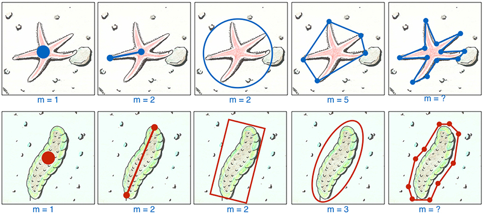
Figure 1. One ROI can be labeled in different ways. We show two example taxa, a starfish and a holothuria, both with five different ways to describe a ROI for them, explained from left to right. The simplest way is to place a point label (far left) which needs only the selection of m = 1 (with m = |r_i|) point (for instance using a mouse, touchpad or a draw pad) to determine r_i. If the size of the ROI is relevant (e.g., to estimate the biomass), the observer can apply different ways to determine r_i with m = 2 or 3 positions (depending on the GUI implementation) using for instance lines, circles, frames, ellipsoids. In some cases, the number of vertices to describe a shape is rather low and constant, so in this case a polygon can be applied for a more detailed size / shape description (see m = 5 for the star fish). If a more detailed size description is need, one may consider to draw a polygon with an arbitrary number of nodes (examples on the far right) which usually causes a much higher work.

The classifications c_i = (c_{i, 1}, …, c_{i, J}) list all J classifications done in J inspections or sessions. Of course, in the majority of annotation projects, the index J is rather low and (J = 1) holds for most of the annotations. Each classification is described by two parameters

$\begin{array}{l}{c}_{i,j}=(\omega ,k)\end{array}$

which are (a) one category⁵ ω from the set of possible categories Ω (ω∈Ω) assigned to the ROI r_i, (b) one observer (i.e., annotating expert) O_k from a group of observers O_k∈{O₁, …, O_K}. Based on these definitions we describe three types of image annotation tasks that are also illustrated in Figure 2.

• FIA: Full image annotation task

In FIA the whole content of an image is classified to one category (e.g., habitat type), i.e., the classifications c_{i, j} are assigned to the entire image I_t (r_i = ∅) and no individual ROI is to be described inside the image.

This kind of an image annotation task is usually performed very quickly because it does not require a mouse interaction to specify the ROI. The most common application scenario for FIA is when time for annotation is limited and a rapid annotation process is necessary (e.g., in live video feed annotation). FIA is also useful to flag entire images as empty (i.e., no ROI of any category ω visible), as not interpretable (e.g., artifacts, sediment cloud) or not of interest for further analysis (e.g., test images acquired on deck of an RV). This flagging process can be conducted prior or alongside a Whole Image Screening annotation (see next task description). Tools that implement FIA often feature pre-defined buttons for each ω (see for instance A.-E. in Figure 2) that only need to be selected to assign a time-coded annotation of category ω regarding the image visible at the time t.

• Whole image screening (WIS)

In a WIS task, the observer has to search for all ROI in an image, which are of relevance. This type of annotation task is the most common in marine image annotation and carried out, when the number (and classifications) of all ROI in an image is to be determined. In many cases, observers need to mark the positions and the contour of the ROI as well, when for instance biomass information is to be estimated for each ROI. Considering the time an observer is spending for one annotation, WIS is on average the most time-consuming task in image annotation since each time spent for one annotation is the sum of the time for search and selection of the pixel group r_i and the time for the classification step to select ω.

The way how to select the ROI is a crucial part of the WIS and needs thorough consideration by the complete group of observers. The final scientific question or the driving hypothesis behind the study is the most important discriminant here: in case abundances of categories ω are targeted, simple point labels [i.e., the ROI description consists of a pixel coordinate r_i = (x_i, y_i)] that do not provide a shape/site description are sufficient; in cases where the extent of individual r_i matters (e.g., for biomass estimates), annotation shapes like lines, rectangles, ellipses, or polygons are required. Apart from the definition of annotation shapes, further consideration is required regarding the placement of the shapes in the images (see Section 4 below for the list of recommendations).

• Single patch classification (SPC)

In a SPC session, a set of ROI from prior collected annotations {A_i} is investigated and classified by the observer O_k who needs to make a decision regarding the acceptance/rejection of ω. This annotation task is much faster than WIS regarding the number of investigated ROI per time. From a methodological perspective SPC could be considered as a “small scale FIA.” The image patches are anyhow by orders of magnitude smaller than the entire images in FIA and a subset of them can be displayed on a screen in a rapid serial visual presentation (i.e., showing one patch at a time and with dynamic updates like in a slideshow) or in a rich gridded visual presentation (i.e., several patches in parallel and static) (see Figure 2 on the right). SPC has seen rare applications in marine image annotation yet [except in case of posterior inspections of annotations obtained by a computer vision system (Schoening et al., 2012b; Osterloff et al., 2016; Schoening et al., under review)] since it needs a sophisticated data base model to represent the annotations ROIs and classifications.

Annotation projects carried out with the so called random points approach can be considered a SPC task, since the observer inspects a given number of randomly set points in an image and classifies the image content at those image points to one category. So the observer can concentrate totally on the classification step.

FIGURE 2

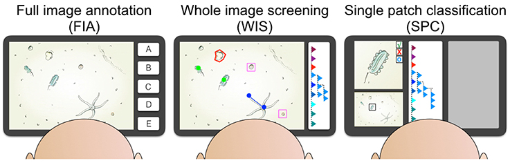
Figure 2. The three different kinds of annotation tasks are illustrated. The full image annotation (FIA) task asks the observer to label an image with one category (for instance A, …, E) based on the content of the complete image. The whole image screening task (WIS) includes searching one image for all instances of one or more taxonomic or morphologic categories and to label this graphically. The categories can for instance be displayed in a hierarchical browser (see right side of the WIS screen). The observer uses different kinds of labels like points (green), lines (blue), frames (pink), or poligons (red). In the rapidly performed sigle patch classification (SPC) single pre-selected individuals are displayed with high resolution and detail and the observer decides to accept the existing label, reject the label or to reset the label (see upper left in the SPC screen). The rest of the screen space can be used to display the entire source image (with the individual highlighted in a black frame, see lower left) and to display other helpful annotation information (gray box).

No matter what kind of annotation task is performed, the whole process can be considered as one signal detector or sensor with the annotations {r_i} as sensor outputs. And like each other sensor, the outputs need to be evaluated regarding the quality of the results which is the subject of Section 3. First, we need to address the problem of collecting a gold standard for a correct annotation of a chosen subset of images that can be used in the quality assessment as a reference.

3. Quality Assessment

In any visual inspection and annotation task, the results should be of a quality, that it allows to include them in a scientific study or in a decision process. In marine image annotation, the concept for a high or low annotation quality is often not clearly defined. To close this gap, this section will describe quality measures for image annotation as well as ways to create reference data sets for comparison, also referred to as gold standards.

3.1. The Gold Standard Issue

In each scenario of annotation quality assessment (see next section) a test set of images with a gold standard annotation result is required. The test set must represent the diversity of input signals and structures monitored which means that each category considered in the study shall be represented with an appropriate number of examples. The gold standard must be accepted by the scientific community to be an acceptable approximation of the ground truth. To acquire a gold standard for a test set of images three different strategies have been applied in the past:

3.1.1. Single Expert

One expert observer visually inspects the test set and performs the annotation task (FIA, WIS, or SPC) and the result is considered the gold standard for this data. This strategy requires an observer with extra ordinary skills and expertise and an evaluation of this experts' intra-observer agreement (see Section 3.2 for details).

3.1.2. Consensus Expert

A number of K observers inspects a test set of images and perform the annotation task. So the number of inspections equals the number of experts, J = K. All the expert observers use the same annotation software, use the same categories and follow the same annotation protocol. It is important that all K observers need to perform independently from each other so none of their classifications is affected by the classification of the other observers. The result lists of annotations c_i from all K observers are compared for each annotation A_i to construct a meta-expert annotation result. To this end, spatially and semantically corresponding annotations from different observers need to be matched and fused to one. This is done algorithmically by searching for annotations that have very close and/or have overlapping region descriptions r_i and have the same category ω assigned. As a result, for each ROI that has been detected and classified by at least one observer a consensus factor γ_i ∈ {1, …, K} is computed, representing the number of observers that have detected and classified this ROI to be from one and the same particular category. The list of all ROI with a consensus factor 1 ≤ γ_i ≤ K above a given threshold is used as the gold standard G. This strategy has been applied for instance in (Nattkemper et al., 2003; Schoening et al., 2012b). The quality of the gold standard can be assessed by evaluating the observers' inter- and intra-observer agreement (see Section 3.2). The latter is of course condition to performing a repetitive experiment of each observer for a subset of the test set.

3.1.3. Ground Truth Data

In the ideal case, a ground truth is available generated with data from other sources. One example from the field of underwater mining is for instance box corer data, i.e., physical sampling from the ground. This procedure is time consuming and has the drawback that it is destructive to some extend. However, on the other hand, the result delivers a very good reference to be applied as gold standard.

3.2. Quality Measures

Many researchers use different terms like accuracy or precision to denote the quality of an annotation process, sometimes even using them in a wrong way or without a concise definition. In this section we will give an overview for quality assessment definitions and methods which are relevant to the marine image annotation problem. To outline the description of the quality measures in a clear way we focus on so called two class problems here. This means that |Ω| = 2 and two categories ω₁ and ω₀ are considered. Extending the quality measures to multi-category problems requires some further considerations. An excellent overview of multi-category quality assessment is given in Sokolova and Lapalme (2009).

As test sets one might consider large collections of image patches like in the SPC scenario (see Section 2 above) or an image set from the sea floor {I_t}, each image showing a different number of instances from this category. The categories could be for instance

a. ω₁ = is_a_sponge and ω₀ = is_no_sponge, or

b. ω₁ = is_starfish_morphotype_A and

ω₀ = is_starfish_morphotype_B, or

c. ω₁ = coral and ω₀ = stressed_coral

We also assume here, that for the test set, a gold standard G is available (see section before) so the decision of an observer O_k can be evaluated to be correct or not. We propose to use and distinguish the following terms to assess the quality of the annotation results obtained for the image collection.

3.2.1. Accuracy

The accuracy describes the ability of an observer to make decisions or classifications that can be considered as correct condition to an available gold standard representing the state-of-the-art knowledge. To assess the accuracy of an annotation, a test set of image data must be provided together with a gold standard (see Section 3.1 before) and the accuracy is usually described by ROC statistics. In ROC the focus is usually put on one particular category and the observer O_k classifies a ROI to be positive (ω₁) or negative (ω₀), i.e., the object belongs to the category or not (see for example a. above). Comparing the results of the observer obtained for a test set with those from a test set's gold standard classification allows to classify each observer result to be a true positive (TP), true negative (TN), false positive (FP), or false negative (FN). The TP for example represent the number of ROIs that were classified to be positive by the observer and in the gold standard. The FP are those ROI that were classified to be positive by the observer but negative in the gold standard.

In the accuracy assessment, the observer's classifications for all ROI / image patches are compared to those in the gold standard reference. The most frequently used ROC parameters computed from these four variables are

$\begin{array}{l}\mathbf{\text{recall}}=\frac{TP}{TP+FN},\mathbf{\text{precision}}=\frac{TP}{TP+FP},\\ \mathbf{\text{specificity}}=\frac{TN}{TN+FP}.& (2)\end{array}$

Sometimes, the first two terms are referred to as sensitivity (= recall) and positive predictive value (= precision) since in some image processing communities these are more popular from their application in medical imaging.

SPC: In SPC, recall and specificity are usually evaluated and sometimes classic ROC plots are drawn, relating recall to (1-specificity). To express the overall performance, the accuracy is computed by

$\begin{array}{ll}\mathbf{\text{ACC}}=\frac{TP+TN}{TP+FP+FN+TN}.& (3)\end{array}$

Other values proposed to represent a singe measure for the observer's accuracy are the harmonic mean (also referred to as F₁-measure):

$\begin{array}{ll}{F}_1=2·\frac{\mathrm{\text{precision }}·\mathrm{\text{ recall}}}{\mathrm{\text{precision }}+\mathrm{\text{ recall}}}& (4)\end{array}$

or the geometric mean (referred to as G-measure):

$\begin{array}{ll}G=\sqrt{\mathrm{\text{precision }}·\mathrm{\text{ recall}}}& (5)\end{array}$

In many applications a separate display and analysis of the recall and precision should maybe be preferred. The kind of losses and costs caused by the different kind of errors [like too many missed objects (i.e., TN) in case of a low recall value or too many FP in case of a low precision] can have rather different impact. Thus, a separate analysis of these two often makes sense. The single valued measures (Equations 3–5) can be rather useful to tune the parameters of software system or to compare the performance in a compact way.

WIS: In a WIS task, the observer's performance is assessed by computing the precision and the recall and relating those to each other. The specificity is usually neglected since the TN, i.e., the number of pixels in the image that have correctly not been labeled as a ROI is by orders of magnitude larger than the FP. Thus, the specificity is usually close to 1.0, i.e., perfect which does not reflect the performance of the observers correctly.

3.2.2. Reproducibility

The ability to reproduce results from an experiment is one corner stone in good scientific practice and must be considered in the development and application of new scientific methods. In the context of marine image annotation this term describes the ability of one observer to either reproduce her/his results or the results of a second observer for the same data set. The reproducibility should be discussed separately from the accuracy, since the significance of an accuracy assessment depends on the availability of an accepted gold standard. But even if such a gold standard is missing, the ability of one observer to reproduce her/his results or the results of a second observer must be shown to demonstrate the potential of an imaging based approach to produce significant results. In fact, if the classification task is very complicated and difficult to perform by the observers due to the image quality, a reproducibility analysis should be carried out before collecting gold standard annotations or should be an integrated part of this procedure.

The reproducibility of an annotation process can be assessed by computing the inter-observer agreement between two observers O_j and O_k, for instance with κ-statistics (Cohen, 1960; Landis and Koch, 1977; Viera and Garrett, 2005). Please note, that the inter-observer agreement between two observers O_k and O_j, is sometimes also referred to as “precision” in other scientific fields such as medicine and clinical research. However, since we use the term “precision” to describe the relation of true positives TP to all positives (TP + FP) (see Equation 2), we propose to use the term “reproducibility” here, since it refers very well to the task of the observer, to reproduce one list of annotations, pre-produced by another observer. Obviously O_j can represent a second result obtained by the same and first observer O_k (i.e., j = k) for the same data set but with some time delay. In this case, such an inter-observer agreement would be referred to as intra-observer agreement.

In κ-statistics, the expected agreement A_e of two observers is estimated and related to the observed agreement A_o. To quantify A_e and A_o an experiment is carried out, where two observers have to classify N samples (e.g., ROI / image patches) to show instances from one chosen category or not or from another category, respectively (see a.–c. above). In Table 1 we show an example for N = 200 of two observers, with n_1k (n_1j) as the number of items classified by the observer O_k (O_j) as ω₁ and n_0k (n_0j) as the number of items classified as ω₀ by the two observers, respectively. The variable n₁₁ represents the number of items both observers have classified as ω₁ and n₀₀ is the number both have classified as ω₀.

TABLE 1

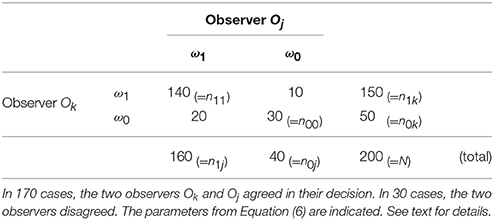
Table 1. The table shows the abundances of classifications for 200 inputs into two categories ω₁ and ω₀.

The expected agreement A_e and the observed agreement A_o are computed by

$\begin{array}{ll}{A}_e=\frac{n_{1k}}{N}·\frac{n_{1j}}{N}+\frac{n_{0k}}{N}·\frac{n_{0j}}{N}\text{\hspace{0.17em}\hspace{0.17em}\hspace{0.17em}\hspace{0.17em}and\hspace{0.17em}\hspace{0.17em}\hspace{0.17em}\hspace{0.17em}}{A}_o=\frac{n_{11}+n_{00}}{N}.& (6)\end{array}$

From the numbers in our example in Table 1 we compute A_e = 0.65 and A_o = 0.85.

Please note, that if we replace one observer O_j by a gold standard G, the observed agreement A_O is identical to the accuracy value (see Equation 3). The κ statistic is computed by

$\begin{array}{l}\kappa =\frac{A_o-A_e}{1-A_e},\kappa \in \left[-1;1\right].\end{array}$

A large value of κ = 1 indicates a perfect agreement, a value of κ = 0 indicates no agreement and κ = −1 a systematic disagreement or contradiction. In the example we get κ = 0.57 which is usually interpreted as a moderate agreement according to the agreement scale proposed in Landis and Koch (1977) and shown in Table 2.

TABLE 2

Table 2. A scale for six levels of agreement assigned to six intervals of κ.

However, in particular situations two problems can occur in κ statistics. First, the expected agreement A_e might just be based on small empirical measurements and the significance of the result can not be estimated without further expensive experiments to measure the variance for κ and a z statistic etc. Second, one can reach a high expected agreement and high observed agreement but a low κ value in the special case, when the abundances for observations of the two categories (like ω₁ and ω₀ in our example) are very unbalanced in the test set. To solve this issue, one has to apply the methods proposed in Feinstein and Cicchetti (1990); Cicchetti and Feinstein (1990).

We propose to distinguish the two terms accuracy and reproducibility in marine image annotation quality assessment, since a high accuracy value must not necessarily point to an excellent observer performance. Consider for instance a test set with non-balanced category distributions and a high a priori probability for one category, so a naive biased observer can reach high accuracy values just by chance. But since the observer would not be able to reproduce the result (since it was based on guessing) the reproducibility is low! The other way round, an observer can make a systematic mistake due to false instructions but the result would be reproducible. So the observer would have a high reproducibility but a low accuracy. Distinguishing these two terms reflect the phenomenon, that decisions of observers are influenced by training (i.e., non-randomness) and experience (i.e., the ability to explain a decision and to reproduce it).

3.2.3. Quantitative Data

In some marine mapping or exploration projects, the aim is to extract quantitative information from the marine images. For large continuous complex shaped structures (like corals, sponges, bacterial mats, etc.) this can be done using grid cells, random point clouds or counting of instances without marking their positions. In this case, the quality of the result is assessed by comparing the extracted quantities with a reference result, also referred to as gold standard or ground truth (see section before). If for instance the quantities are extracted for each image I_t from an image collection acquired in one or more dives {_{It}(t = 1, …, nt)} the labeling process represents a mapping I_t↦F(t) with F(t) being the quantity or abundance of item from one category in the image I_t. Since the image collection is collected with a moving platform (ROV, AUV, OFOS) or with a stationary camera the values F(t) can be treated as a time series and the correlation coefficient is used to compare the result with the gold standard G(t) (see for instance (Purser et al., 2009)). If each image is considered as one experimental run, statistical methods such as ANOVA can be applied (see for instance Morrison et al., 2012).

4. RecoMIA: Recommendations for Marine Image Annotation

We separate the entire annotation project into four phases of preparation, annotation, quality assessment, and workshops. The recommendations for carrying out the study are organized accordingly.

Phase I: Preparation

R1: Discuss who will label the data (i.e. {O_k}). It should be clear, who will work on the annotation project, who can invest how much time.

R2: Discuss and decide what you want to annotate (i.e., the image collection {I_t} and the categories Ω). Do not think that existing ontologies and definitions will help too much. Most ontologies/categories for biological subjects were developed by scientists who collected samples/cut the samples and inspected them under the microscope. Many morphological criteria can not be applied in image analysis. It is important to limit the number of categories in Ω = {ω} in a meaningful way because each further ω slows down the mental decision process to pick a category for an annotation A_i and thus the whole annotation process. Because most marine image annotation is conducted on unseen data, Ω usually changes over time to incorporate new categories or by discarding others that do not occur in the images. In case further Ω shall be considered (e.g., to discriminate live and dead specimen of the same category ω), all annotations of this category need to be assessed again (ideally with an SPC or, much slower, by a WIS). Also discuss which version of an image you annotate. This could be the original image, a lens-distortion corrected image, or a color-corrected image. Make sure that all observers use the same image data. If artifacts, as shadows or scientific gear, prevent annotation in parts of the images, make sure that each observer knows which region within images to annotate.

R3: Discuss and decide how you want to label (FIA, WIS, SPC). Because most marine image annotation is conducted on unseen data, Ω usually changes over time. But changing the annotation type (FIA, WIS, SPC), the parametric ROI description r_i (for example changing from a circle shape to an ellipsoid shape or to a line) or Ω after the image annotation finished can also become very time consuming. Consider for instance the case of a finished abundance assessment, using FIA or point marker based WIS, a biomass estimate is targeted: this would require to specify the ROI description r_i for each A_i by screening all images again. Define how to place the annotation markers for WIS tasks explicitely. Markers could be set at the head of individuals or in the center of mass. This point is crucial to be able to assess annotation quality (see Figure 1).

R4: Organize a focus group workshop in advance. The term focus group is used in social sciences and project management to refer to the addressed user (here observer) group in the context of a tool development. The entire group defined in R1. shall meet in front of a screen and annotate a set of test images together. This is very important since it is the only chance to harmonize the different visual models of the fauna/objects/events of interest. This step is essential and can be combined with R1-R3.

R5: Create a set of gold standard annotations during or following the focus group.

R6: Discuss if it is appropriate to keep zoom, i.e., the pixel scale of the image display on the same level when screening images. In many cases a resolution of 1:1 should be selected (1 pixel in the image is displayed by 1 pixel of the monitor). In some cases observer agreement will increase when all observers use the same resolution when screening the images. However, in other cases, the observers need to change the zoom while inspecting the images since they need to intergrate large scale information in the decision process. Nevertheless, this shall be discussed.

R7: Circulate a summary of the discussion and decisions around as a reference to consult during the annotation session. The summary should include a set of example images of each known category to be annotated in the data set. Of course in many exploration studies only a limited number of those are known beforehand.

Phase II: Annotation Session

R8: Try to apply chunking, i.e., to divide the annotation task in sub tasks by dividing the categories into groups of similar appearance or similar morphology to increase efficiency and effectiveness. For one observer, chunking can be implemented in the taxonomical domain by annotating each morphological group after the other. This means that for instance in a first chunk you label all star fishes and all sponges in the next chunk. This will have the effect that you sharpen your eyes for the little differences between similar looking star fishes (i.e., items from one chunk) and that the classification accuracy and reproducibility increases. The drawback is that you have to label the same image several times, each time for different chunks, i.e., groups of ω with similar visual features.

Regarding all observers O, a different way of chunking can also be implemented by letting the group of observers on the beginners level annotate at a low level of taxonomic detail (e.g., using crowd sourcing to simply define ROI without classification). Afterwards the observers on the expert level refine the classifications to a more detailed taxonomic level (for instance using SPC).

R9: If possible have example images of the category ω visible while annotating this category (see recommendation 5. above).

R10: Try to limit the visual / auditory distractions to a minimum so it is easier to focus. Dim the lights and adjust your monitor brightness to keep your eyes from getting tired. Also, not doing anything else is the best. Switch off your email notifications and mobile phone. If you want to listen to music go for something that puts you in a good mood and does not capture your attention (e.g., by listening to lyrics).

R11: Take breaks after 60 min of annotating (latest). Human cognition performance goes down in a monitoring task after 60 min.

Remember: Humans are not suited for image annotation tasks. The visual system developed by evolution (not by design) so inspecting still images from almost unknown environments with physical conditions different to humans every-day environment is very difficult.

Phase III: Quality Assessment

R12: Use SPC to check your own annotations as well as your colleagues' annotations.

R13: Inter-observer agreement: Subsets of the data should be annotated by at least two observers. This is one of two factors to show reproducibility and provide annotation data suitable for high impact publications.

R14: Intra-observer agreement: Parts of the data should be annotated by each observer two times (with a delay of at least 48 h) to study the observer's reproducibility.

Note: It is a common observation, that the inter-/intra observer agreement is very similar. If the intra-observer agreement is much better, often the observers have different degrees of experience. Sometimes the two observers just had a misunderstanding regarding the decisions made following recommendations R2 and R3. above and just annotated different categories or the same category but in a different way.

Phase IV: Workshop

R15: Repeat the focus group meetings regularly to discuss observations made during the annotation sessions as well as the annotation quality of the observers. Eventually update O, I, and Ω, and note the updates and the discussion protocol in a further reference document.

5. Discussion

In this paper we have given a review on available methods to analyze the annotation performance of different observers when manually annotating images from underwater environments. Of course, these methods can be applied to compare the performance of a group of observers, to compare the performance of one observer for the same image data with different pre-processings or to compare the performance of a computer vision system with human observer's performance.

One option to enhance the process of visual interpretation could be to extend parametric description of an annotation (Equation 1) with a confidence value p (p ∈ [0, 1]) that represents the observer's degree of belief in her/his classification of this ROI to the category ω. In case of an algorithmic classification, such a confidence value can be computed from the classifier output. In the more usual case of an annotation done by human observer, this p-value must be entered by the observer, which would of course increase the work load considering situations with a large number of ROIs per image. Another problem would be the fact, that different observers shall have different scaling routines for setting p. Consequently, an additional workshop for the discussion of standards in this regard and the collection of reference ROI examples for different p intervals would be required. This might be one reason, why in the majority of studies, such a confidence value of human observers is not recorded, i.e., is set to a constant p = 1. However, in some projects it may be important to represent this degree of belief since a broader spectrum of observers my be integrated in the annotation process (for instance in citizen science projects).

Accurately defined annotation schemes will allow to assess limits and prospects of marine imaging as a robust sensor. The multitude of camera platforms allows to acquire image data from varying altitudes and in varying view angles. Variations in the recorded visual signal due to attenuation and scattering are the consequence. While images with a large field of view can be acquired from high altitudes, annotation of objects in such images may be aggravated due to limited color information, limited contrast, and limited resolution. To find a trade-off between a large visual footprint and a good annotation quality, at sufficient level of category detail, is a challenge for the near future.

From our point of view the most important contribution of this manuscript is the list of recommendations. In the last years we have experienced, that the quality of the annotations (assessed with inter-/intra-observer agreements and different kind of gold standards) was not so much dependent on the level of scientific experience but more on the way the annotation study has been carried out. This is of course not surprising when looking at the highly standardized way pathologists evaluate their tissue slides for instance. Maybe some of our 15 recommendations may not be applicable in some scenarios, however it may be helpful for some observers to even recognize that these factors have an effect on the performance as well and this may guide them in identifying other factors in their study.

Author Contributions

TN, TS, and JO created and discussed the content of the review and wrote the manuscript. TN is responsible for the graphics/artwork.

Conflict of Interest Statement

The authors declare that the research was conducted in the absence of any commercial or financial relationships that could be construed as a potential conflict of interest.

Acknowledgments

This work was supported by the Bundesministerium für Wirtschaft und Energie (BMWI, FKZ 03SX344A) and Bundesministerium für Bildung und Forschung (BMBF, FKZ 03F0707C).

Footnotes

1. ^NICAMS. NIWA Image Capture Analysis & Management System. Available online at: https://nzoss.org.nz/projects/nicams.

2. ^VARS. Video Annotation and Reference System (VARS). Available online at: http://www.mbari.org/vars/.

3. ^CATAMI. Collaborative and Automated Tools for Analysis of Marine Imagery CATAMI. Available online at: http://catami.org.

4. ^SQUIDLE. Available online at: http://squidle.acfr.usyd.edu.au/.

5. ^In the field of machine learning or pattern recognition the term class is more frequently used than category. However, since the term class usually refers to a level in biological taxonomy we choose to use the term category in this paper but will use classification as the term for assigning a category to an ROI.

References

Abdul Ghani, A. S., and Mat Isa, N. A. (2014). Underwater image quality enhancement through composition of dual-intensity images and Rayleigh-stretching. SpringerPlus 3:757. doi: 10.1186/2193-1801-3-757

PubMed Abstract | CrossRef Full Text | Google Scholar

Ancuti, C., Ancuti, C. O., Haber, T., and Bekaert, P. (2012). “Enhancing underwater images and videos by fusion,” in Computer Vision and Pattern Recognition (CVPR), 2012 IEEE Conference on (Providence, RI), 81–88. doi: 10.1109/CVPR.2012.6247661

CrossRef Full Text

Beijbom, O., Edmunds, P., Kline, D., Mitchell, B., and Kriegman, D. (2012). “Automated annotation of coral reef survey images,” in Computer Vision and Pattern Recognition (CVPR), 2012 IEEE Conference on, 1170–1177.

PubMed Abstract | Google Scholar

Beijbom, O., Edmunds, P. J., Roelfsema, C., Smith, J., Kline, D. I., Neal, B. P., et al. (2015). Towards automated annotation of benthic survey images : variability of human experts and operational modes of automation. PLoS ONE 10:e0130312. doi: 10.1371/journal.pone.0130312

PubMed Abstract | CrossRef Full Text | Google Scholar

Bryson, M., Johnson-Roberson, M., Pizarro, O., and Williams, S. B. (2015). True color correction of autonomous underwater vehicle imagery. J. Field Robot. doi: 10.1002/rob.21638. [Epub ahead of print].

CrossRef Full Text | Google Scholar

Chambah, M., Semani, D., Renouf, A., Courtellemont, P., and Rizzi, P. (2003). “Underwater color constancy: enhancement of automatic live fish recognition,” in Proceedings SPIE, Vol. 5293, Color Imaging IX: Processing, Hardcopy, and Applications, 157. doi: 10.1117/12.524540

CrossRef Full Text | Google Scholar

Chiang, J. Y., Chen, Y., and C. (2012). Underwater image enhancement by wavelength compensation and dehazing. IEEE Trans. Image Process. 21, 1756–1769. doi: 10.1109/TIP.2011.2179666

PubMed Abstract | CrossRef Full Text | Google Scholar

Cicchetti, D. V., and Feinstein, A. R. (1990). High agreement but low kappa: II. resolving the paradoxes. J. Clin. Epidemiol. 43, 551–558.

PubMed Abstract | Google Scholar

Cohen, J. (1960). A coefficient of agreement for nominal scales. Educ. Psychol. Meas. 20, 37–46.

Culverhouse, P., Williams, R., Reguera, B., Herry, V., and Gonzalez-Gil, S. (2003). Do experts make mistakes? A comparison of human and machine identification of dinoflagellates. Mar. Ecol. Prog. Ser. 247, 17–25. doi: 10.3354/meps247017

CrossRef Full Text | Google Scholar

Delaney, D., Sperling, C., Adams, C., and Leung, B. (2008). Marine invasive species: validation of citizen science and implications for national monitoring networks. Biol. Invasions 10, 117–128. doi: 10.1007/s10530-007-9114-0

CrossRef Full Text | Google Scholar

Eustice, R., Pizarro, O., Singh, H., and Howland, J. (2002). “UWIT: underwater image toolbox for optical image processing and mosaicking in MATLAB,” in Proceedings of the 2002 International Symposium on Underwater Technology (Tokyo), 141–145.

Feinstein, A. R., and Cicchetti, D. V. (1990). High agreement but low kappa: I. the problems of two paradoxes. J. Clin. Epidemiol. 43, 543–549.

PubMed Abstract | Google Scholar

Franzoni, C., and Sauermann, H. (2014). Crowd science: the organization of scientific research in open collaborative projects. Res. Policy 43, 1–20. doi: 10.1016/j.respol.2013.07.005

CrossRef Full Text | Google Scholar

Gracias, N., and Santos-Victor, J. (2000). Underwater video mosaics as visual navigation maps. Comput. Vis. Image Understand. 79, 66–91. doi: 10.1006/cviu.2000.0848

CrossRef Full Text

Greiner, M., Pfeiffer, D., and Smith, R. D. (2000). Principles and practical application of the receiver-operating characteristic analysis for diagnostic tests. Prev. Vet. Med. 45, 23–41. doi: 10.1016/S0167-5877(00)00115-X

PubMed Abstract | CrossRef Full Text | Google Scholar

Iqbal, K., Odetayo, M., James, A., Salam, R. A., and Hj Talib, A. Z. (2010). “Enhancing the low quality images using unsupervised colour correction method,” in Systems Man and Cybernetics (SMC), 2010 IEEE International Conference on (Istanbul), 1703–1709. doi: 10.1109/ICSMC.2010.5642311

CrossRef Full Text

Kocak, D., and Caimi, F. (2005). The current art of underwater imaging–with a glimpse of the past and vision of the future. Mar. Technol. Soc. J. 39, 5–26. doi: 10.4031/002533205787442576

CrossRef Full Text | Google Scholar

Kohler, K., and Gill, S. (2006). Coral point count with excel extensions (CPCe): a visual basic program for the determination of coral and substrate coverage using random point count methodology. Comput. Geosci. 32, 1259–1269. doi: 10.1016/j.cageo.2005.11.009

CrossRef Full Text | Google Scholar

Krupinski, E. A., Johnson, J. P., Jaw, S., Graham, A. R., and Weinstein, R. (2012). Compressing pathology whole-slide images using a human and model observer evaluation. J. Pathol. Inform. 3, 607–622. doi: 10.4103/2153-3539.95129

PubMed Abstract | CrossRef Full Text | Google Scholar

Lakhani, K., Jeppesen, L., Lohse, P., and Panetta, J. (2006). The Value of Openness in Scientific Problem Solving. Working paper, Harvard Business School, Boston.

Google Scholar

Landis, J. R., and Koch, G. G. (1977). The measurement of observer agreement for categorical data. Biometrics 33, 159–74.

PubMed Abstract | Google Scholar

Lusted, L. (1971). Signal detectability and medical decision making. Science 171, 1217–1219.

PubMed Abstract | Google Scholar

Lusted, L. (1984a). Decision making studies in patient management. N. Engl. J. Med. 284, 416–424.

PubMed Abstract | Google Scholar

Lusted, L. (1984b). ROC recollected. Med. Decis. Making 4, 131–135.

Google Scholar

MacLeod, N., Benfield, M., and Culverhouse, P. (2010). Time to automate identification. Nature 467, 154–155. doi: 10.1038/467154a

PubMed Abstract | CrossRef Full Text | Google Scholar

Marcon, Y., Ratmeyer, V., Kottmann, R., and Boetius, A. (2015). “A participative tool for sharing, annotating and archiving submarine video data,” in OCEANS 2015 - MTS/IEEE Washington, IEEE, 1–7.

Google Scholar

Metz, C. (1986). ROC methology in radiologic imaging. Invest. Radiol. 21, 720–733.

PubMed Abstract | Google Scholar

Morrison, J., Ruzicka, R., Colella, M., Brinkhuis, V., Lunz, K., Kidney, J., et al. (2012). “Comparison of image-acquisition technologies used for benthic habitat monitoring,” in Proceedings of the 12th International Coral Reef Symposium (Cairns, QLD).

Google Scholar

Nattkemper, T. W., Twellmann, T., Schubert, W., and Ritter, H. (2003). Human vs. machine: evaluation of fluorescence micrographs. Comput. Biol. Med. 33, 31–43. doi: 10.1016/S0010-4825(02)00060-4

PubMed Abstract | CrossRef Full Text | Google Scholar

Ontrup, J., Ehnert, N., Bergmann, M., and Nattkemper, T. W. (2009). “BIIGLE-Web 2.0 enabled labelling and exploring of images from the Arctic deep-sea observatory HAUSGARTEN,” in OCEANS, IEEE, 1–7.

Google Scholar

Orfao, A., Schmitz, G., Brando, B., Ruiz-Arguelles, A., Basso, G., Braylan, R., et al. (1999). Clinically useful information provided by the flow cytometric immunophenotyping of hematological malignancies: current status and future directions. Clin. Chem. 45, 1708–1717.

PubMed Abstract | Google Scholar

Osterloff, J., Nilssen, I., and Nattkemper, T. W. (2016). A computer vision approach for monitoring the spatial and temporal shrimp distribution at the love observatory. Methods Oceanogr. doi: 10.1016/j.mio.2016.03.002. [Epub ahead of print].

CrossRef Full Text | Google Scholar

Osterloff, J., Schoening, T., Bergmann, M., Durden, J. M., Ruhl, H., Nattkemper, T. W., et al. (2014). “Ranking color correction algorithms using cluster indices,” in Computer Vision for Analysis of Underwater Imagery (CVAUI), 2014 ICPR Workshop on, IEEE, 41–48.

Panetta, K., Gao, C., and Agaian, S. (2015). Human-visual-system-inspired underwater image quality measures. IEEE J. Ocean. Eng. 1–11. doi: 10.1109/JOE.2015.2469915

CrossRef Full Text | Google Scholar

Petit, F., Capelle-Laize, A. S., and Carre, P. (2009). “Underwater image enhancement by attenuation inversionwith quaternions,” in 2009 IEEE International Conference on Acoustics, Speech and Signal Processing (Taipei), 1177–1180. doi: 10.1109/ICASSP.2009.4959799

CrossRef Full Text

Pican, N., Trucco, E., Ross, M., Lane, D. M., Petillot, Y., and Tena Ruiz, I. (1998). “Texture analysis for seabed classification: co-occurrence matrices vs. self-organizing maps,” in OCEANS '98 Conference Proceedings, Vol. 1 (Nice), 424–428. doi: 10.1109/OCEANS.1998.725781

CrossRef Full Text

Pizarro, O., Williams, S., and Colquhoun, J. (2009). “Topic-based habitat classification using visual data,” in Proceedings of IEEE OCEANS'09 (Bremen), 1–8.

Purser, A., Bergmann, M., Lundalv, T., Ontrup, J., and Nattkemper, T. (2009). Use of machine-learning algorithms for the automated detection of cold-water coral habitats: a pilot study. Mar. Ecol. Prog. Ser. 397, 241–251. doi: 10.3354/meps08154

CrossRef Full Text | Google Scholar

Purser, A., Ontrup, J., Schoening, T., Thomsen, L., Tong, R., Unnithan, V., et al. (2013). Microhabitat and shrimp abundance within a norwegian cold-water coral ecosystem. Biogeosciences 10, 5779–5791. doi: 10.5194/bg-10-5779-2013

CrossRef Full Text | Google Scholar

Rylance, R. (2015). Global funders to focus on interdisciplinarity. Nature 525, 313–315. doi: 10.1038/525313a

PubMed Abstract | CrossRef Full Text | Google Scholar

Schettini, R., and Corchs, S. (2010). Underwater image processing: state of the art of restoration and image enhancement methods. EURASIP J. Adv. Signal Process. 2010, 1–15. doi: 10.1155/2010/746052

CrossRef Full Text | Google Scholar

Schoening, T., Bergmann, M., and Nattkemper, T. (2012a). “Investigation of hidden parameters influencing the automated object detection in images from the deep seafloor of the HAUSGARTEN observatory,” in Oceans, 2012 (IEEE), 1–5.

Schoening, T., Bergmann, M., Ontrup, J., Taylor, J., Dannheim, J., Gutt, J., et al. (2012b). Semi-automated image analysis for the assessment of megafaunal densities at the Arctic deep-sea observatory HAUSGARTEN. PLoS ONE 7:e38179. doi: 10.1371/journal.pone.0038179

PubMed Abstract | CrossRef Full Text | Google Scholar

Schoening, T., Ehnert, N., Ontrup, J., and Nattkemper, T. (2009). “BIIGLE tools - a Web 2.0 approach for visual bioimage database mining,” in IV 09 - International Conference on Information Visualization (Barcelone).

Schoening, T., Kuhn, T., Bergmann, M., and Nattkemper, T. (2015). DELPHI - fast and adaptive computational laser point detection and visual footprint quantification for arbitrary underwater image collections. Front. Mar. Sci. 2:20. doi: 10.3389/fmars.2015.00020

CrossRef Full Text | Google Scholar

Shneiderman, B. (2008). Copernican challenges face those who suggest that collaboration, not computation are the driving energy for socio-technical systems that characterize Web 2.0. Science 319, 1349–1350. doi: 10.1126/science.1153539

PubMed Abstract | CrossRef Full Text | Google Scholar

Singh, H., Roman, C., Pizarro, O., Eustice, R., and Can, A. (2007). Towards high-resolution imaging from underwater vehicles. Int. J. Robot. Res. 26, 55–74. doi: 10.1177/0278364907074473

CrossRef Full Text | Google Scholar

Sokolova, M., and Lapalme, G. (2009). A systematic analysis of performance measures for classification tasks. Inform. Process. Manag. 45, 427–437. doi: 10.1016/j.ipm.2009.03.002

CrossRef Full Text | Google Scholar

Trucco, E., and Olmos-Antillon, A. (2006). Self-tuning underwater image restoration. Ocean. Eng. IEEE J. 31, 511–519. doi: 10.1109/JOE.2004.836395

CrossRef Full Text | Google Scholar

Tusa, E., Reynolds, A., Lane, D., Robertson, N., Villegas, H., and Bosnjak, A. (2014). “Implementation of a fast coral detector using a supervised machine learning and gabor wavelet feature descriptors,” in Sensor Systems for a Changing Ocean (SSCO), 2014 IEEE, 1–6.

Viera, A. J., and Garrett, J. M. (2005). Understanding interobserver agreement: the kappa statistic. Family Med. 37, 360–363.

PubMed Abstract | Google Scholar

Waldrop, M. (2008). Science 2.0. Sci. Am. 298, 68–73. doi: 10.1038/scientificamerican0508-68

PubMed Abstract | CrossRef Full Text | Google Scholar

Wang, R., Wang, Y., Zhang, J., and Fu, X. (2015). “Review on underwater image restoration and enhancement algorithms,” in Proceedings of the 7th International Conference on Internet Multimedia Computing and Service, ICIMCS15 (New York, NY: ACM), 56:1–56:6.

Wuchty, S., Jones, B. F., and Uzzi, B. (2007). The increasing dominance of teams in production of knowledge. Science 316, 1036–1039. doi: 10.1126/science.1136099

PubMed Abstract | CrossRef Full Text | Google Scholar

Yang, M., and Sowmya, A. (2015). An underwater color image quality evaluation metric. Image Process. IEEE Trans. 24, 6062–6071. doi: 10.1109/TIP.2015.2491020

PubMed Abstract | CrossRef Full Text | Google Scholar

Zuiderveld, K. (1994). “Contrast limited adaptive histogram equalization,” in Graphics Gems IV, ed P. S. Heckbert (San Diego, CA: Academic Press Professional, Inc.), 474–485.

Zweig, H. M., and Campbell, G. (1993). Receiver-operating characteristic (ROC) plots: a fundamental evaluation tool in clinical medicine. Clin. Chem. 39, 561–577.

PubMed Abstract | Google Scholar