Voltammetric Investigation of Hydrothermal Iron Speciation

Introduction

Iron (Fe) is an essential micronutrient for all marine organisms. Although Fe is the fourth most abundant element in the earth's crust (Hans Wedepohl, 1995), dissolved Fe (dFe, <2 μm) concentrations are low in the world's oceans, typically <1 nM in the deep ocean and even lower (<0.2 nM) in surface waters, due to microbial uptake and the low solubility of Fe(OH)₃ in seawater (Johnson et al., 1997; Maldonado and Price, 2001; Liu and Millero, 2002). Iron exists in two oxidation states in seawater: the bioavailable and relatively soluble Fe(II), occurring naturally in chemically reducing conditions such as hydrothermal vent fluids, and Fe(III), which is the dominant form in oxidized seawater (Landing and Westerlund, 1988). Since the bioavailable and soluble Fe(II) is rapidly oxidized to thermodynamically stable and insoluble Fe(III) in oxic waters, microorganisms have adapted to natural Fe limitation by producing metal chelating organic molecules. These organic ligands, for example siderophores, are able to protect Fe(III) from precipitation and may be reduced by microorganisms to bioavailable Fe(II) complexes (Kraemer, 2004; Gledhill and Buck, 2012). Recent studies by Gledhill et al. (2015) and Stockdale et al. (2016) showed that a large portion of DOM also binds Fe(III), which may be an additional and more general passive, not biologically active, control on Fe concentrations in the oceans.

Until recently, atmospheric dust inputs and fluxes from the continental margins were believed to be the major Fe sources for the surface ocean (Moore et al., 2004). However, hydrothermal vents, which host fluid Fe concentrations up to seven orders of magnitude greater than the typical deep ocean, have recently been shown to play an important role in the deep ocean Fe budget (Bennett et al., 2008; Saito et al., 2013; German et al., 2015; Hatta et al., 2015; Resing et al., 2015), and this has implications for surface ocean dFe concentrations (Tagliabue et al., 2010). Due to their high acidity and fluid temperatures above 400°C, metals such as Fe are leached out of the host rock as the fluid circulates through the basaltic crust. Most of this dissolved Fe is directly precipitated around the vent outlets as Fe-sulfides or is oxidized to Fe oxyhydroxides upon mixing with oxic seawater (German et al., 1991; Rudnicki and Elderfield, 1993), and a substantial portion of these mineral phases may exist in the operationally defined “dissolved” fraction as colloids or nanoparticles (Yücel et al., 2011; Hawkes et al., 2013a, 2014; Gartman et al., 2014). These nanoparticles might be transported away from vents in the dissolved fraction, making an important contribution to the global oceanic Fe budget. A second mechanism by which hydrothermal Fe may be stabilized after venting into the ocean is via chelation with organic ligands, stabilizing Fe(III) in the dissolved phase, which can then be transported away from the vent site (Bennett et al., 2008; Toner et al., 2009; Sander and Koschinsky, 2011; Hawkes et al., 2013a). Iron that is available for natural organic ligands is the part of total Fe that is not precipitated or stabilized by inorganic compounds, called labile Fe. In this study, we are assuming that labile Fe is organically bound only and not inorganic colloids, which would then be non-labile. Hydrothermally derived dFe is transported over thousands of kilometers away from its source into the open ocean (Fitzsimmons et al., 2014; Resing et al., 2015). The relative importance of the inorganic vs. organic stabilization may have important consequences in the long-term stability and bioavailability of the hydrothermal Fe, and the relative contribution of these stabilization mechanisms remains highly uncertain. In surface and oxic deep waters, organic complexation dominates the speciation of Fe, since most (>98%) dissolved species are bound to strong organic ligands increasing Fe solubility and therefore also the total dissolved Fe concentration in the world's oceans (Gledhill and van den Berg, 1994; Rue and Bruland, 1995; Wu and Luther, 1995; Boyd et al., 2010), whereas inorganic colloids are often important at redox boundaries such as in hydrothermal plumes and oxidized sediment pore waters (Homoky et al., 2009; Hawkes et al., 2014). Studying the sources, sinks as well as the chemical speciation of hydrothermal Fe is therefore a crucial step in order to understand the bioavailability and cycling of Fe in our oceans.

The hydrothermal island arc system at the Coriolis Troughs, near the islands of Vanuatu and east of New Caledonia has not previously been studied with respect to organic Fe complexation. Studying the role of island arc systems with respect to hydrothermal metal contribution to the water column is important, since these vents make up ~9% of global hydrothermal flux (Baker et al., 2008), are often rich in trace metals (de Ronde et al., 2011; Leybourne et al., 2012), and often occur at shallower water depths compared to Mid Oceanic Ridge (MOR) systems—potentially having a more direct impact on surface water chemistry (Hawkes et al., 2014). To broaden the knowledge and understanding on global hydrothermal dFe speciation and distribution, we determined the total and chemically labile iron concentrations (dFe, Fe_lab) together with corresponding Fe ligand concentrations ([L]) and their iron-binding strengths (logK_FeL,Fe³⁺) at the hydrothermal vent fields in the Coriolis Troughs, New Hebrides Island Arc.

Materials and Methods

Samples

All hydrothermal fluid samples were collected within the Coriolis Troughs in the year 2013 during research cruise SO 229. The Coriolis Troughs lie east of the Erromango and Tana islands, and are situated in the Vanuatu backarc basin east of the southern New Hebrides island arc. The system is composed of three major depressions orientated NNW-SSE, the Vate Trough in the North, the Erromango Trough in the middle, and the Futuna Trough in the South (Figure 1). Since 1969, the troughs themselves have been intensively studied, however only little is known about the hydrothermal system within the troughs (Greene and Exon, 1988; Price et al., 1993; Iizasa et al., 1998; Nasemann, 2015; Schmidt et al. under review). During a research cruise in 2001, McConachy et al. (2005) discovered a new large hydrothermal vent field, the “Nifonea vent field” in the central Vate Trough, east of Nifonea Ridge.

FIGURE 1

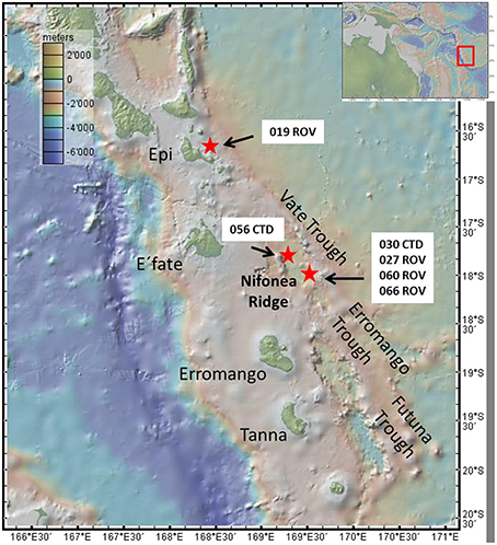
Figure 1. Map showing the New Hebrides Island arc with the islands of Vanuatu, the three Trough systems and the Nifonea Ridge as well as Epi Caldera, including all sampling stations. Map was created using GeoMapApp.

Except for sample 19 ROV 06 (taken at the Epi Caldera) all other hydrothermal fluid samples were taken within the Nifonea vent field. Additional to several black smokers and diffuse vent fields; a non-buoyant hydrothermal plume was detected above the Nifonea vent field by turbidity anomalies in the water column and was sampled using the on-board conductivity-temperature-depth (CTD) rosette water sampler at five different water depths. Figure 2 shows four different sampled vent sites; diffuse venting at Epi Caldera and two black smokers as well as one high-temperature clear vent fluid in the Nifonea vent field. For the direct sampling of hydrothermal fluids from the high-temperature vents, the fully remotely controlled flow-through system KIPS (Kiel Pumping System, KIPS-4; Garbe-Schönberg et al., 2006) entirely made of polytetrafluoroethylene (PTFE) and high-purity titanium was deployed on the ROV KIEL 6000. Samples were collected via a titanium nozzle, which was connected to four PTFE sampling bottles, one liter each. Parallel to the nozzle is an on-line high-temperature sensor monitoring the temperature at the point of sampling, which helps in detecting the most focused vent outlets. Within the Nifonea vent field, maximum temperatures of 368°C were measured at single black smoker vent outlets (Haase, 2013; Schmidt et al., under review). Figure 2A shows the sampling titanium nozzle with the high-temperature sensor attached to it, while sampling a diffuse hydrothermal vent field at the Epi Caldera. Before filling the sampling tube and sample bottles, both were rinsed with the hydrothermal fluid for several minutes. This KIPS sampling technique is fully remotely controlled on board the research vessel and therefore allows a detailed fluid sampling in defined areas. In addition to the KIPS system, three metal-free, acid cleaned Niskin bottles were deployed at the front porch of the ROV to sample the mixing zones of pure fluid and seawater, the buoyant plume.

FIGURE 2

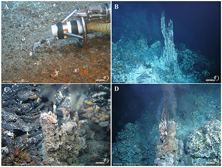
Figure 2. (A) Diffuse, low temperature hydrothermal venting at Epi Caldera (19 ROV 06). (B) Black smoker, at Nifonea ridge (27 ROV 14, 15, and 16). (C) Clear, high temperature (348°C) vent at Nifonea ridge (60 ROV 01 and 02). (D) Black smoker (170°C) at Nifonea ridge (66 ROV 05). (Pictures taken by ROV KIEL 6000, GEOMAR Kiel, Germany). Panel (A) also shows the use of the KIPS system with the titanium nozzle and parallel high-temperature sensor.

In total, one non-buoyant hydrothermal plume (five samples) and nine different hydrothermal fluid samples have been taken for dFe, Fe_lab, and [L] analysis (Table 1).

TABLE 1

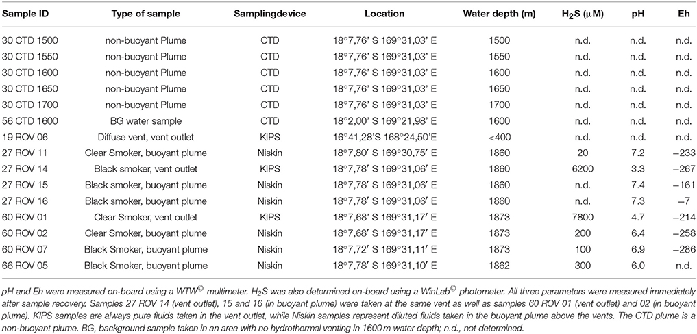
Table 1. Overview on hydrothermal samples taken for Fe speciation.

Methods

Most Fe measurements were performed by voltammetric analysis using a 757 VA Computrace (Metrohm) at Jacobs University Bremen, Germany. The three-electrode configuration included a hanging mercury drop electrode (HMDE) as the working electrode, a double junction Ag/AgCl/3 M KCl reference electrode, and a glassy carbon counter electrode. Since most fluid samples taken by the ROV KIEL 6000 were believed to have dFe concentrations in μM range, all ROV samples were additionally analyzed using a Spectro Ciros Vision ICP-OES at Jacobs University Bremen.

On board SO 229, samples were filtered (0.2 μM) and acidified (suprapure HCl, pH 2) if used for metal determination or frozen directly after filtration if used for speciation. Samples were stored in acid-cleaned LDPE or HDPE fluorinated bottles. At shore, a 10 ppm Fe stock solution was prepared in suprapure 0.1 M HCl (using the 1000 ppm Fe single element standard, Joint Ventures). Iron standard solutions for voltammetric analysis (10 and 1 μM) were prepared daily by diluting the 10 ppm Fe stock solution with ultrapure deionized water (DI, 18.2 MΩ/cm). An aqueous stock solution of 0.1 M salicylaldoxime (SA) from Sigma-Aldrich was prepared in suprapure 0.1 M HCl and stored at 4°C. SA standard solutions (10 and 1 mM) were regularly prepared from the 0.1 M SA stock solution. A borate buffer was mixed out of 1 M boric acid and 0.35 M suprapure ammonia. To remove trace metals, this solution was passed over a chelating ion exchange resin (chelex 100, BioRad) before use.

Total dissolved Fe (dFe) was determined in 10 mL of the acidified sample, with the addition of an artificial ligand (SA; final concentration 25 μM; Rue and Bruland, 1995; Buck and Bruland, 2007; Buck et al., 2007; Abualhaija and van den Berg, 2014). After the SA addition, the sample was allowed to stand for about 2 h, before the pH was adjusted to ~8.15 using suprapure NH₃ and the borate buffer (10 mM final concentration). DFe concentrations in each sample were then determined by adsorptive cathodic stripping voltammetry (AdCSV), which detects the electrochemically-active complex FeSA using standard addition method. All sample and titration vials were conditioned typically three times prior to each measurement.

Voltammetric parameters were modified from (Abualhaija and van den Berg 2014). This includes purging of the sample with compressed air (instead of N₂) at 1 bar, deposition at −0.05 V with an initial deposition time of 120 s (this was later adjusted to shorter times due to high Fe concentrations) and a cathodic scan from −0.05 to−0.8 V using the differential pulse (DP) mode. Every measurement was repeated three times for quality control and reproducibility. Additionally, the seawater reference material for trace metals NASS-6 from the National Research Council Canada was measured along the samples for dFe as quality control. The analytical error for NASS-6 was within the range of ±5 % of the reference value.

For labile Fe (Fe_lab) measurements, the sample was thawed at 4°C overnight. Ten milliliters of the sample were pipetted into an already conditioned PTFE titration vessel and equilibrated overnight at ~pH 8.15 (borate buffer, 10 mM final concentration) and 100 μM SA. Due to high dFe concentrations, ROV samples were first diluted with ultrapure deionized water in the same salinity as the sample. The next day, regular Fe standard additions were made with 10 min equilibration time after each addition, using the same voltammetric parameters as for dFe. The chemically labile Fe that we are measuring is the fraction of iron in the sample as FeSA complex. This means that it dissociated from its previous complex with natural ligands to be available to our artificial ligand SA under these conditions, i.e., it is labile. Curvature in the standard addition data points suggested that, despite the high SA concentration of 100 μM, there was still competition between some natural ligands and SA at low Fe additions (Figure 3). To estimate concentration and binding strength of possible Fe-complexing ligands we made five additions of Fe. Plotting this data in ProMCC, using the complete complexation-fitting model, one-ligand model, resulted in reasonable Fe binding ligand concentrations (Omanović et al., 2015).

FIGURE 3

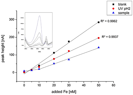
Figure 3. Typical titration curve exemplarily chosen for sample 27 ROV 11 with Fe standard additions at pH 8.15 and 100 μM SA for the reagent blank, a UV digested sample at pH 2 and the regular sample. The sample without any Fe addition was equilibrated overnight. The voltammogram shows the standard additions of Fe to sample 27 ROV 11.

To validate this data, a regular titration with 12 Fe additions equilibrated overnight was prepared for two of the non-buoyant plume samples (30 CTD 1500 and 30 CTD 1650). Twelve aliquots (10 ml each) of each sample were separated in 15 ml PTFE vials. The borate buffer (final concentration 10 mM), as well as increasing Fe concentrations at approximately logarithmic steps are given to each sample, ranging from 0 to 300 nM, depending on the expected ligand concentration. After 2 h of equilibration, the artificial ligand SA was added at a concentration of 25 μM. All 12 sample aliquots were allowed to equilibrate overnight and subsequently analyzed the next day, using the same parameters as for the dFe (Table 2). Since results of the standard addition titration and the regular titration were very similar, we decided to show and work with the results of the standard addition method in this study.

TABLE 2

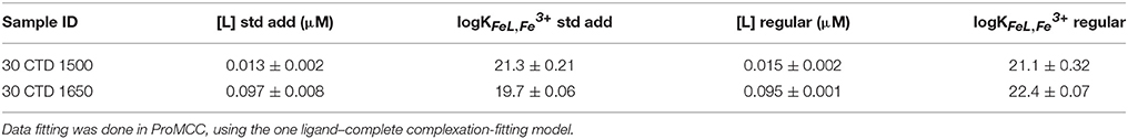
Table 2. Comparison of [L] and logK_FeL,Fe³⁺ data obtained with a standard addition titration and a regular classic titration with 12 separate Fe additions and overnight equilibration.

As a second method proof, we also measured a pH 2 UV digested sample and a reagent blank (used for dilution) using the same procedure and voltammetric parameters as for the regular samples. These results did not show the curvature in the beginning at low Fe additions, confirming that the curvature is not a methodological artifact but truly sample related (Figure 3).

Results

Total Dissolved Fe and Labile Fe Concentrations

Our non-buoyant plume samples had dFe concentrations between 10 and 30 nM, compared to a background concentration of 7 nM (Table 3). These concentrations represent an approximate dilution of vent fluids of ~38,000. Samples 30 CTD 1500 (10 nM Fe) and 30 CTD 1700 (10 nM Fe) taken directly above and beneath the plume show only little enriched dFe concentrations compared to the background seawater sample. The three samples taken within the plume core are enriched compared to regular seawater and follow the turbidity signal of the CTD water sampler (Figure 4), which can be used as a tracer for hydrothermal plumes. The highest peak in turbidity also shows the highest dFe concentration for the hydrothermal plume. These observations agree with a recent study on the same plume (Nasemann, 2015).

TABLE 3

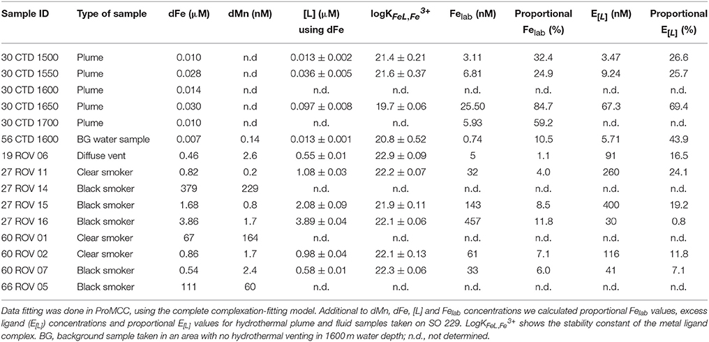
Table 3. Iron speciation data for hydrothermal plume and fluid samples taken on SO 229.

FIGURE 4

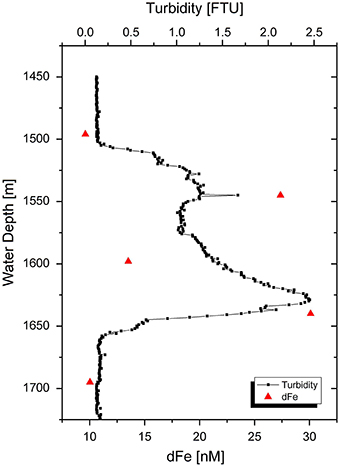
Figure 4. Turbidity signal of non-buoyant plume 30 CTD above the Nifonea vent field. Red triangles display dFe concentrations in the approximate depths of sampling. Bottles were closed in 1500, 1550, 1600, 1650, and 1700 m water depth.

For the vent fluids taken at the seafloor, our samples had dFe concentrations in a much wider range; between 0.46 μM for sample 19 ROV 06 taken from a diffuse vent up to 379 μM for black smoker sample 27 ROV 14 taken directly in the vent outlet. It can be observed that both KIPS samples 27 ROV 14 and 60 ROV 01 that are also characterized by highest H₂S and lowest pH values of all samples, show higher dFe concentrations than the samples taken with Niskin bottles above the same vents, which in general would represent more diluted fluids. However, one sample, 66 ROV 05, taken ~1 m above the vent outlet had an unusually high dFe concentration (111 μM) although taken with a Niskin bottle and not the KIPS system. Sample 19 ROV 06, also collected using KIPS had a dFe concentration of 0.46 μM, much lower than all other KIPS samples, which can be explained by the fact that this site is a diffuse vent field, as opposed to a high temperature clear or black smoker as all other fluid samples. Additionally, clear smoker samples 27 ROV 11, 60 ROV 01, and 60 ROV 02 had lower dFe concentrations than comparable samples taken at black smokers.

The proportion of chemically labile Fe (Fe_lab) in dFe increased during development of the buoyant hydrothermal plume from values between 1 and 11.8% near the vent mouth to values between 25 and 85% in the non-buoyant plume. The term “labile Fe” is defined as the dFe which is bound to SA after equilibration with 100 μM SA overnight at room temperature (α_FeSA = 3.39 × 10¹², α_FeSA2 = 1.58 × 10¹²). This is quite a high overall side reaction coefficient for out-competing natural ligands, but high dFe and [L] concentrations required a higher than normal SA concentration. The fact that a curvature was still found (Figure 3) in the standard addition curve indicated some ligand exchange, thus validating the SA concentration used. After overnight equilibration, we made five standard additions with 10 min equilibration time after each addition and used the data to estimate the Fe binding strength of the competing ligands. Due to the observed curvature, the determined Fe_lab concentrations should be considered minimum estimates (Table 3). In general, a strong linear correlation can be observed between dFe and Fe_lab for all fluid samples as shown in Figure 5.

FIGURE 5

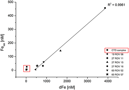
Figure 5. Labile Fe (Fe_lab) plotted against dissolved Fe (dFe) for all ROV samples collected within the buoyant plume and CTD samples (within red square) collected within the non-buoyant plume.

Iron Binding Ligand Concentrations

Concentrations for Fe binding ligands [L] within the non-buoyant hydrothermal plume ranged between 13 and 97 nM, with stability constants (logK_FeL,Fe³⁺) varying from 19.7 to 21.6. Generally, the “plume core” samples had higher ligand concentrations than the ones beneath and above the inner plume. Sample 30 CTD 1500 taken above the plume had a very similar [L] concentration as the background seawater sample. As already shown for dFe and Fe_lab, a strong correlation can be observed when plotting dFe against [L] (Figure 6). Since all ROV samples plot slightly above the 1:1 diagonal, we can assume that all available Fe is being complexed. The CTD samples seem to plot on the diagonal. Fe_lab and [L] show a correlation of R² = 0.972 (Figure 7).

FIGURE 6

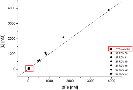
Figure 6. Fe binding ligand ([L]) concentrations plotted against total dissolved Fe (dFe) for all ROV samples collected within the buoyant hydrothermal plume, and CTD samples collected within the non-buoyant plume. Dashed line represents the 1:1 diagonal.

FIGURE 7

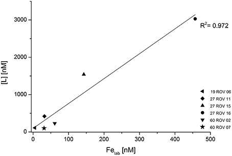
Figure 7. Fe binding ligand concentrations ([L]) plotted against labile Fe (Fe_lab) for all hydrothermal samples collected with the ROV.

Iron binding ligand data for the samples collected in the buoyant plume very close to the high temperature vents had concentrations ranging from 0.55 up to 3.89 μM or from 0.10 up to 3.03 μM depending on the initial Fe concentration used for calculations (dFe or Fe_lab, respectively), while more diluted fluids had higher [L] concentrations (Table 4). Stability constants for the buoyant plume samples ranged from logK_FeL,Fe³⁺ 21.9 up to 22.9 or from logK_FeL,Fe³⁺ 19.7 up to 21.9, again, depending on the initial Fe concentration used for calculation (dFe or Fe_lab, respectively). The general trend shows that the higher the dFe concentration, the higher the [L] concentration. When calculating the excess ligand (E_[L]) concentrations and proportional E_[L] for all samples, an opposite trend to the Fe_lab values can be found in buoyant plume samples (Table 3). The most diluted buoyant plume sample 27 ROV 16 had the highest proportional Fe_lab values but lowest E_[L]; a trend which is not continued in the non-buoyant plume samples, where Fe_lab values rather seem to mimic E_[L] values.

TABLE 4

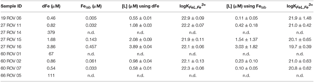
Table 4. Comparison of the different calculated ligand characteristics [L] and logK_FeL,Fe³⁺ for all ROV samples using dFe or Fe_lab as initial iron concentrations.

Discussion

In this study, we adapted the traditional titration method (Rue and Bruland, 1995) due to problems arising from the high Fe concentrations and inorganic matrix of the hydrothermal samples. Our original goal was simply to assess the concentration of labile Fe in each sample (Hawkes et al., 2013b), but curvature in the standard additions allowed us to estimate some strong Fe binding ligand characteristics. Despite a short 10-minequilibration time after each Fe addition and a high concentration of SA (100 μM), some Fe in the samples was complexed by natural ligands. The classic titration worked satisfactorily for the non-buoyant hydrothermal plume samples, which we carried out for two exemplarily chosen samples to compare results of both methods (Table 2). The two methods gave similar results for [L], but on one occasion quite different results for the conditional binding strength, logK. This may be due to the equilibration time, which may favor certain types of ligand according to the coordination mechanism. Regardless, both methods were able to extract some labile Fe from natural complexes.

A second consideration was whether to use the total dissolvable Fe concentration (dFe) in the calculation of the ligand characteristics or to use the labile Fe concentration (e.g., Hawkes et al., 2013b). If some dFe is present as inorganic colloids which we suppose here do not participate in the equilibrium, the ligand concentration and strength would be overestimated by using dFe in the calculations. However, if some ligand complexes which do participate are too strong in the detection window employed, these factors will be underestimated. We calculated the ligand parameters using both iron concentrations for all ROV samples, which had relatively low Fe_lab values with a maximum of 11.8%, giving us a minimum and maximum estimate for [L], which vary greatly, particularly in logK (Table 4). The results gathered from the use of dFe are probably unrealistic, as it is generally accepted that a significant portion of hydrothermal dFe is inorganically bound in mineral matrices (Yücel et al., 2011; Hawkes et al., 2013a, 2014; Gartman et al., 2014). We also know that our determined value of Fe_lab is an underestimation, due to the curvature in the standard additions, but these ligand parameters are probably a more realistic estimation of the Fe speciation in the plume. The high ligand concentration and fairly low binding coefficient are in line with previous results gathered by reverse titration (Hawkes et al., 2013b), and may result from complexation of Fe with less specific binding groups on DOM than in surface waters (Gledhill et al., 2015; Stockdale et al., 2016).

Fe Speciation within the Buoyant and Non-buoyant Hydrothermal Plume

A speciation study for five single layers of the 30 CTD non-buoyant hydrothermal plume above the Nifonea vent field showed highly elevated dFe and [L] concentrations compared to the surrounding seawater, especially in the plume center. Consistently present excess ligand concentrations between 25 and 69% indicate that all available Fe (Fe_lab) is being complexed and stabilized. A recent study by (Nasemann 2015) showed that dFe concentrations mimic those of particulate Fe, indicating nearly equal amounts of dissolved and particulate Fe in the non-buoyant plume. These findings are also reflected by the turbidity signal. However, they found that particulate Fe concentration decreased above plume depths (>1500 m), dFe continued to be elevated above the plume, which may indicate incomplete particle formation at the upper end of the plume, or stabilization of the dissolved species. Our findings that dFe and [L] concentration increase toward the plume core are in good agreement with the findings of Bennett et al. (2008) and also support the theory that these high dFe and [L] concentrations are not coming from the mixing with open ocean water or the true vent fluid but rather from diffuse venting adjacent to the high temperature vents.

All plume samples as well as the background seawater sample were taken with the research vessel's own CTD water sampler, which was not an official trace metal clean CTD and might explain the relatively high dFe background concentrations of 7 nM, which would then also apply for the non-hydrothermal plume samples. However, plume samples are still enriched in dFe compared to the background sample.

Calculating [L] with dFe as initial Fe concentration, the buoyant plume shows [L] concentrations being consistently in excess compared to dFe concentrations (Table 4). However, this might be specific to the Nifonea hydrothermal vent field with its many high temperature vents, such as 27 ROV, where dFe and [L] concentrations in μM range were measured in the fluids on the seafloor. Using Fe_lab values for calculations, [L] concentrations are higher than Fe_lab but consistently lower than dFe, which is in agreement with previous studies (Bennett et al., 2008; Hawkes et al., 2013a; e.g., Buck et al., 2015).

The ratio of Fe_lab:dFe was characteristically higher in the samples taken from black smoker chimneys than those taken at diffuse venting sites or clear smokers, suggesting that sub-surface processes removed labile Fe or preferentially led to non-labile forms of Fe, such as sulfide nanoparticles and oxidized colloids. In the buoyant hydrothermal plume, the proportion of labile Fe increased as the plume was diluted, indicating either that Fe species became more labile over the timescale of plume formation sampled (~hours), or that non-labile forms of dFe were preferentially removed. The latter explanation is more likely, as colloidal oxy-hydroxide particles are likely to gradually aggregate into species larger than the “dissolved” cutoff (>0.2 μm; Honeyman and Santschi, 1989; Hawkes et al., 2014).

The Source and Nature of Fe Ligand Complexes

Iron binding ligand concentrations around the vent outlets were distributed very heterogeneously varying from 0.55 up to 3.89 μM or 0.10 up to 3.03 μM, depending on the initial Fe concentration used for calculation; however, seem to be highly related to the corresponding dFe or Fe_lab concentration (Figures 6, 7). The fact that elevated dFe and Fe_lab concentrations in the buoyant plume also led to higher [L] concentrations, gives reason for the assumption that these ligands have their source close to these vent outlets. When calculating the proportion of labile Fe, it can be observed that for the buoyant plume, only between 1.1 and 11.8% are actually chemically labile, while Fe_lab increases with plume dilution. Interesting are samples 27 ROV 14, 15, and 16, which are all from the same vent, with 27 ROV 16 being a more diluted fluid than 27 ROV 15, while 27 ROV 14 represents the actual high temperature vent fluid. While 27 ROV 14 shows dFe concentrations up to 379 μM, a lot of dFe is probably lost as particulate or colloidal Fe sufides or oxyhydroxides directly after seawater mixing as shown in sample 27 ROV 15 (1.68 μM dFe). The even higher diluted fluid 27 ROV 16, shows higher Fe_lab and higher [L] concentrations than 27 ROV 15, indicating that the ligand source could be present within the plume, as bacteria, which actively produce organic ligands or organo-sulfur compounds (Toner et al., 2009), or adjacent to the vent site in areas of diffuse fluid flow (Bennett et al., 2008). The diffuse vent sample 19 ROV 06, taken with the KIPS system, shows lowest dFe and lowest [L] concentrations and at the same time also the lowest value of Fe_lab:dFe, with only 1.1%, which we would rather expect from a pure hydrothermal fluid sample (Yücel et al., 2011). Additionally, pure hydrothermal fluids, sampled directly out of the vent outlet, have low concentrations of complex organic matter, so we would not expect to find organic ligands in these samples (Hawkes et al., 2015; McCollom et al., 2015). However, an important fraction (up to 11.8%) of dFe in the early buoyant plume was chemically labile and in equilibrium with high concentrations of natural chelating ligands, as indicated by their competition for added Fe during titration (Figure 3). UV digestion at pH 2 followed by pH neutralization and measurement showed a decrease in dFe and Fe_lab and an increase in sensitivity. This may indicate a loss of Fe to inorganic particles after destruction of organic molecules, and a loss of organic competition for added Fe, respectively (Figure 3).

The close relationship between [L] and dFe concentrations in the buoyant plume (Figure 6) suggests either that the ligands have a similar source as the Fe (Bennett et al., 2008) or that the observed voltammetric behavior of dFe is an inherent feature of Fe in organic rich seawater (Hawkes et al., 2013a, 2015), due to the diverse functionality of the organic mixture (Gledhill et al., 2015; Stockdale et al., 2016) and the gradual and possibly weak aggregation of oxy-hydroxide and other colloidal Fe phases (Honeyman and Santschi, 1989; Mackey and Zirino, 1994). This strong correlation between dFe and [L] was already observed in previous studies (Buck and Bruland, 2007; Buck et al., 2007; Lannuzel et al., 2015). Regardless of their source or identification, these organic ligands seem to control the solubility and therefore also the bioavailability of dFe (Buck et al., 2007). Buck and Bruland (2007) also suggested that dFe might be required for the production of these ligands. All of these previous studies focused on different water types including estuarine waters, river plumes, surface waters, and Antarctic sea ice. To our knowledge, no other studies have yet been reported on dFe, Fe_lab, and [L] in hydrothermal buoyant plume samples and since our samples show a very strong correlation of dFe and [L] (Figure 6), these results confirm previous outcomes and imply that also in hydrothermal plumes, [L] might control the concentration of dFe. The additional good correlation between Fe_lab and [L] (Figure 7) gives reason for the suggestion that [L] might also control Fe_lab in theses environments or vice versa.

Highest stability constant and thereby the highest binding strength of the [L] complex was measured in sample 19 ROV 06 (logK_FeL,Fe³⁺ = 22.9 or 21.9, using dFe or Fe_lab for calculation, respectively), a diffuse vent fluid, however sampled with KIPS and thereby a quite pure fluid. All other ROV samples analyzed for [L] and logK are sampled within the buoyant plume and had values between logK_FeL,Fe³⁺ = 19.7 and logK_FeL,Fe³⁺ = 22.3, signifying for strong ligands (Gledhill and Buck, 2012). Stability constants for the non-buoyant hydrothermal plume, calculated using dFe as initial iron concentration were lower with values between logK_FeL,Fe³⁺ = 19.7 and logK_FeL,Fe³⁺ = 21.6. Since we used the standard addition method to determine [L] and logK-values, we only had five data points available, which leads to greater uncertainty and possibly an overestimation of the logK-value. However, since there is no other comparable data published for high temperature vent fluids, our data might serve as a first approach, leaving room for further method development and more data analysis.

During the analysis we used SA as an artificial ligand for all samples and purged with air. In this case a possible reverse titration is not a good option as the FeSA peak would decrease with increasing SA concentration (Abualhaija and van den Berg, 2014). To validate our data, a reverse titration using 1-nitroso-2-naphthol (NN) as an artificial ligand as demonstrated by Hawkes et al. (2013b) would be a reasonable next step.

Distribution of Fe from Hydrothermal Vents

Our speciation results suggest that nearly all of the hydrothermally derived dFe in the buoyant plumes is strongly complexed or part of nano-particles and colloids, and not chemically labile in the time scale of 1 day during plume dispersal. In the true vent fluids, most of the Fe will occur as Fe(II), however, only meters away from where the fluid gets mixed with oxic seawater, Fe(III) will be the dominant oxidation state (Sander and Koschinsky, 2011). Our oxidation half-life calculations of Fe (t_1∕2 = 1.1 h; calculated using equations by Millero et al., 1987; Statham et al., 2005) confirmed that Fe should be in the Fe(III) form in all the non-buoyant and most of the buoyant plume samples. Since these fluids are very high in sulfide and the oxidation half-life is very short, a high fraction of Fe is most likely bound as pyrite nanoparticles and Fe oxy-hydroxide colloids, rather than by organic stabilizing ligands (Luther et al., 2001; Yücel et al., 2011; Hawkes et al., 2013a). In high temperature vents, it has been shown that about 5–25% of hydrothermally derived dFe is released into the deep ocean in the form of nano particulate pyrite, while these nanoparticles can behave like dissolved metals, by not settling and thereby being transported away from the vent source into the plume or even further (Yücel et al., 2011; Gartman et al., 2014), contributing significantly to the global oceanic dFe budget, which could also be the case for the vents in the Nifonea vent field. However, since we did not analyze for pyrite or other nano-particulate Fe-species, we can only say that results from our study show evidence for <0.2 μm particles containing Fe. In addition to these inorganic stabilization mechanisms, we also found that the proportion of organic Fe binding ligands participating in Fe speciation is higher in the non-buoyant plume than in the buoyant plume, as indicated by high Fe_lab (up to 84.7% in the non-buoyant plume) and [L], providing a large fraction of dFe which may be transported over a longer distance as [L] complexes. Since the fraction of Fe_lab increased with plume dilution, a process removing the colloids or transferring them into the labile phase must occur in the transition zone between the early buoyant plume and the non-buoyant plume. Our results conform well to the growing body of literature which suggests that iron binding ligands are intricately linked with transport of Fe from hydrothermal vent fields (Bennett et al., 2008; Sander and Koschinsky, 2011; Resing et al., 2015). In terms of the various modeling scenarios presented in Resing et al. (2015), we found little evidence to suggest that the hydrothermal flux of organic ligands was significantly greater than that of dFe, and rather support the theory that only a portion of dFe transport from hydrothermal vent fields is in the form of organic complexes, with the rest present as non-chemically labile nano-particles and colloids.

Conclusion

Here, we report for the first time apparent Fe-binding organic ligand concentrations in μM range for a high temperature hydrothermal vent field. Iron binding ligand concentrations were found in excess compared to labile Fe concentrations for all samples in the buoyant and non-buoyant plume of the high temperature vents. [L] is highly dependent on dFe, which suggests that at least some of the organic Fe stabilizing ligands might originate near the hydrothermal vents where most of the dFe is being released. For the buoyant hydrothermal plumes, however, most of the dFe is present as nano- and colloidal mineral phases, and is not chemically labile. The fact that more diluted buoyant plume samples had a higher proportion of Fe_lab and [L] concentrations provides support for the theory that the ligands are most likely supplied from areas of diffuse flow adjacent to the high temperature vent sites (Bennett et al., 2008).

Our results suggest that also the Nifonea vent field is releasing dissolved and stabilized Fe into the ocean, which might exist in the water column for a long time span. Since the Nifonea vent field plume was detected between 1500 and 1700 m water depth, it is unlikely that dFe supplied by this system reaches the photic zone (<200 m), as the studied area is not located within an upwelling region. However, in shallower island arc settings as the Lesser Antilles Island Arc, hydrothermal discharge often occurs as diffuse venting in very shallow water depths (~10 m) rather than as direct emanating fluids, which, looking at our results in this study, suggests that hydrothermal Fe may have a more direct impact on the surface water chemistry. Other settings, such as the Kermadec Arc, hosting several high temperature hydrothermal vents in different water depths from 1600 to only 200 m (de Ronde et al., 2007), would also be very interesting to study with respect to Fe speciation and long term stabilized dFe transport into the deep-ocean and especially surface waters.

Author Contributions

First author CK was solely responsible for collection and analysis of all hydrothermal samples mentioned in this study. Interpretation of the data was mainly performed by CK and JH with discussions with SS and AK. All authors contributed to the final version of this manuscript.

Conflict of Interest Statement

The authors declare that the research was conducted in the absence of any commercial or financial relationships that could be construed as a potential conflict of interest.

Acknowledgments

We gratefully acknowledge the BMBF (German Federal Ministry of Education and Research) for funding the project 03G 0229. Thanks are due to Captain D. Korte, the officers and the crew of the RV SONNE as well the ROV KIEL 6000 crew (GEOMAR Kiel) for their excellent co-operation and effort during the cruise. We also like to thank Dr. D. Garbe-Schönberg for fluid sampling with the KIPS system during SO 229. We acknowledge C. van den Berg and P. Nasemann for helpful discussions. CK's Ph.D. project is funded by MARUM, University Bremen through the Excellence Cluster “The Ocean in the Earth System” (GB4). We are thankful to the two reviewers for their insightful comments.

References

Abualhaija, M. M., and van den Berg, C. M. G. (2014). Chemical speciation of iron in seawater using catalytic cathodic stripping voltammetry with ligand competition against salicylaldoxime. Mar. Chem. 164, 60–74. doi: 10.1016/j.marchem.2014.06.005

CrossRef Full Text | Google Scholar

Baker, E. T., Embley, R. W., Walker, S. L., Resing, J. A., Lupton, J. E., Nakamura, K., et al. (2008). Hydrothermal activity and volcano distribution along the Mariana arc. J. Geophys. Res. 113, B08S09. doi: 10.1029/2007JB005423

CrossRef Full Text | Google Scholar

Bennett, S. A., Achterberg, E. P., Connelly, D. P., Statham, P. J., Fones, G. R., and German, C. R. (2008). The distribution and stabilisation of dissolved Fe in deep-sea hydrothermal plumes. Earth Planet. Sci. Lett. 270, 157–167. doi: 10.1016/j.epsl.2008.01.048

CrossRef Full Text | Google Scholar

Boyd, P. W., Mackie, D. S., and Hunter, K. A. (2010). Aerosol iron deposition to the surface ocean—Modes of iron supply and biological responses. Mar. Chem. 120, 128–143. doi: 10.1016/j.marchem.2009.01.008

CrossRef Full Text | Google Scholar

Buck, K. N., and Bruland, K. W. (2007). The physicochemical speciation of dissolved iron in the Bering Sea, Alaska. Limnol. Oceanogr. 52, 1800–1808. doi: 10.4319/lo.2007.52.5.1800

CrossRef Full Text | Google Scholar

Buck, K. N., Lohan, M. C., Berger, C. J. M., and Bruland, K. W. (2007). Dissolved iron speciation in two distinct river plumes and an estuary: Implications for riverine iron supply. Limnol. Oceanogr. 52, 843–855. doi: 10.4319/lo.2007.52.2.0843

CrossRef Full Text | Google Scholar

Buck, K. N., Sohst, B., and Sedwick, P. N. (2015). The organic complexation of dissolved iron along the U.S. GEOTRACES (GA03) North Atlantic Section. Deep Sea Res. II Top. Stud. Oceanogr. 116, 152–165. doi: 10.1016/j.dsr2.2014.11.016

CrossRef Full Text | Google Scholar

de Ronde, C. E. J., Baker, E. T., Massoth, G. J., Lupton, J. E., Wright, I. C., Sparks, R. J., et al. (2007). Submarine hydrothermal activity along the mid-Kermadec Arc, New Zealand: large-scale effects on venting. Geochem. Geophys. Geosys. 8. doi: 10.1029/2006gc001495

CrossRef Full Text | Google Scholar

de Ronde, C. E. J., Massoth, G. J., Butterfield, D. A., Christenson, B. W., Ishibashi, J., Ditchburn, R. G., et al. (2011). Submarine hydrothermal activity and gold-rich mineralization at Brothers Volcano, Kermadec Arc, New Zealand. Miner. Depos. 46, 541–584. doi: 10.1007/s00126-011-0345-8

CrossRef Full Text | Google Scholar

Fitzsimmons, J. N., Boyle, E. A., and Jenkins, W. J. (2014). Distal transport of dissolved hydrothermal iron in the deep South Pacific Ocean. Proc. Natl. Acad. Sci. U.S.A. 111, 16654–16661. doi: 10.1073/pnas.1418778111

PubMed Abstract | CrossRef Full Text

Garbe-Schönberg, D., Koschinsky, A., Ratmeyer, V., Jähmlich, H., and Westernstroeer, U. (2006). KIPS–a new multiport valve-based all-teflon fluid sampling system for ROVs. Geophys. Res. Abstr. 8, 07032.

Google Scholar

Gartman, A., Findlay, A. J., and Luther, G. W. (2014). Nanoparticulate pyrite and other nanoparticles are a widespread component of hydrothermal vent black smoker emissions. Chem. Geol. 366, 32–41. doi: 10.1016/j.chemgeo.2013.12.013

CrossRef Full Text | Google Scholar

German, C. R., Fleer, A. P., Bacon, M. P., and Edmond, J. M. (1991). Hydrothermal scavenging at the Mid-Atlantic Ridge: radionuclide distributions. Earth Planet. Sci. Lett. 105, 170–181. doi: 10.1016/0012-821X(91)90128-5

CrossRef Full Text | Google Scholar

German, C. R., Legendre, L. L., Sander, S. G., Niquil, N., Luther, G. W., Bharati, L., et al. (2015). Hydrothermal Fe cycling and deep ocean organic carbon scavenging: model-based evidence for significant POC supply to seafloor sediments. Earth Planet. Sci. Lett. 419, 143–153. doi: 10.1016/j.epsl.2015.03.012

CrossRef Full Text | Google Scholar

Gledhill, M., Achterberg, E. P., Li, K., Mohamed, K. N., and Rijkenberg, M. J. A. (2015). Influence of ocean acidification on the complexation of iron and copper by organic ligands in estuarine waters. Mar. Chem. 177, 421–433. doi: 10.1016/j.marchem.2015.03.016

CrossRef Full Text | Google Scholar

Gledhill, M., and Buck, K. N. (2012). The organic complexation of iron in the marine environment: a review. Front. Microbiol. 3:69. doi: 10.3389/fmicb.2012.00069

PubMed Abstract | CrossRef Full Text

Gledhill, M., and van den Berg, C. M. G. (1994). Determination of complexation of iron(III) with natural organic complexing ligands in seawater using cathodic stripping voltammetry. Mar. Chem. 47, 41–54. doi: 10.1016/0304-4203(94)90012-4

CrossRef Full Text | Google Scholar

Greene, H. G., and Exon, N. F. (1988). Acoustic stratigraphy and hydrothermal activity within Epi Submarine Caldera, Vanuatu, New Hebrides Arc. Geo-Marine Lett. 8, 121–129. doi: 10.1007/BF02326088

CrossRef Full Text | Google Scholar

Haase, K. M. (2013). Shipboard Scientists, 2013. Volcanism, Hydrothermal Activity and Vent Biology in the Coriolis Troughs. New Hebrides Island Arc. RV Sonne SO-229 Cruise Report.

Hans Wedepohl, K. (1995). The composition of the continental crust. Geochim. Cosmochim. Acta 59, 1217–1232. doi: 10.1016/0016-7037(95)00038-2

CrossRef Full Text | Google Scholar

Hatta, M., Measures, C. I., Wu, J., Roshan, S., Fitzsimmons, J. N., Sedwick, P., et al. (2015). An overview of dissolved Fe and Mn distributions during the 2010–2011 U.S. GEOTRACES north Atlantic cruises: GEOTRACES GA03. Deep Sea Res. II Top. Stud. Oceanogr. 116, 117–129. doi: 10.1016/j.dsr2.2014.07.005

CrossRef Full Text | Google Scholar

Hawkes, J. A., Connelly, D. P., Gledhill, M., and Achterberg, E. P. (2013a). The stabilisation and transportation of dissolved iron from high temperature hydrothermal vent systems. Earth Planet. Sci. Lett. 375, 280–290. doi: 10.1016/j.epsl.2013.05.047

CrossRef Full Text | Google Scholar

Hawkes, J. A., Connelly, D. P., Rijkenberg, M. J. A., and Achterberg, E. P. (2014). The importance of shallow hydrothermal island arc systems in ocean biogeochemistry. Geophys. Res. Lett. 41, 942–947. doi: 10.1002/2013GL058817

CrossRef Full Text | Google Scholar

Hawkes, J. A., Gledhill, M., Connelly, D. P., and Achterberg, E. P. (2013b). Characterisation of iron binding ligands in seawater by reverse titration. Anal. Chim. Acta 766, 53–60. doi: 10.1016/j.aca.2012.12.048

PubMed Abstract | CrossRef Full Text | Google Scholar

Hawkes, J. A., Rossel, P. E., Stubbins, A., Butterfield, D., Connelly, D. P., Achterberg, E. P., et al. (2015). Efficient removal of recalcitrant deep-ocean dissolved organic matter during hydrothermal circulation. Nat. Geosci. 8, 856–860. doi: 10.1038/ngeo2543

CrossRef Full Text | Google Scholar

Homoky, W. B., Severmann, S., Mills, R. A., Statham, P. J., and Fones, G. R. (2009). Pore-fluid Fe isotopes reflect the extent of benthic Fe redox recycling: evidence from continental shelf and deep-sea sediments. Geology 37, 751–754. doi: 10.1130/G25731A.1

CrossRef Full Text | Google Scholar

Honeyman, B. D., and Santschi, P. H. (1989). A Brownian-pumping model for oceanic trace metal scavenging: evidence from Th isotopes. J. Mar. Res. 47, 951–992. doi: 10.1357/002224089785076091

CrossRef Full Text | Google Scholar

Iizasa, K., Kawasaki, K., Maeda, K., Matsumoto, T., Saito, N., and Hirai, K. (1998). Hydrothermal sulfide-bearing Fe-Si oxyhydroxide deposits from the Coriolis Troughs, Vanuatu backarc, southwestern Pacific. Mar. Geol. 145, 1–21. doi: 10.1016/S0025-3227(97)00112-6

CrossRef Full Text | Google Scholar

Johnson, K. S., Gordon, R. M., and Coale, K. H. (1997). What controls dissolved iron concentrations in the world ocean? Mar. Chem. 57, 137–161. doi: 10.1016/S0304-4203(97)00043-1

CrossRef Full Text | Google Scholar

Kraemer, S. M. (2004). Iron oxide dissolution and solubility in the presence of siderophores. Aquat. Sci. Res. 66, 3–18. doi: 10.1007/s00027-003-0690-5

CrossRef Full Text | Google Scholar

Landing, W. M., and Westerlund, S. (1988). The solution chemistry of iron(II) in Framvaren Fjord. Mar. Chem. 23, 329–343. doi: 10.1016/0304-4203(88)90102-8

CrossRef Full Text | Google Scholar

Lannuzel, D., Grotti, M., Abelmoschi, M. L., and van der Merwe, P. (2015). Organic ligands control the concentrations of dissolved iron in Antarctic sea ice. Mar. Chem. 174, 120–130. doi: 10.1016/j.marchem.2015.05.005

CrossRef Full Text | Google Scholar

Leybourne, M. I., de Ronde, C. E. J., Wysoczanski, R. J., Walker, S. L., Timm, C., Gibson, H. L., et al. (2012). Geology, hydrothermal activity, and sea-floor massive sulfide mineralization at the rumble ii west mafic caldera. Econ. Geol. 107, 1649–1668. doi: 10.2113/econgeo.107.8.1649

CrossRef Full Text | Google Scholar

Liu, X., and Millero, F. J. (2002). The solubility of iron in seawater. Mar. Chem. 77, 43–54. doi: 10.1016/S0304-4203(01)00074-3

CrossRef Full Text | Google Scholar

Luther, G. W., Rozan, T. F., Taillefert, M., Nuzzio, D. B., Di Meo, C., Shank, T. M., et al. (2001). Chemical speciation drives hydrothermal vent ecology. Nature 410, 813–816. doi: 10.1038/35071069

PubMed Abstract | CrossRef Full Text | Google Scholar

Mackey, D. J., and Zirino, A. (1994). Comments on trace metal speciation in seawater or do “onions” grow in the sea? Anal. Chim. Acta 284, 635–647. doi: 10.1016/0003-2670(94)85068-2

CrossRef Full Text | Google Scholar

Maldonado, M. T., and Price, N. M. (2001). Reduction and transport of organically bound iron by Thalassiosira Oceanica (Bacillariophyceae). J. Phycol. 37, 298–310. doi: 10.1046/j.1529-8817.2001.037002298.x

CrossRef Full Text | Google Scholar

McCollom, T. M., Seewald, J. S., and German, C. R. (2015). Investigation of extractable organic compounds in deep-sea hydrothermal vent fluids along the Mid-Atlantic Ridge. Geochim. Cosmochim. Acta 156, 122–144. doi: 10.1016/j.gca.2015.02.022

CrossRef Full Text | Google Scholar

McConachy, T. F., Arculus, R. J., Yeats, C. J., Binns, R. A., Barriga, F. J. A. S., McInnes, B. I. A., et al. (2005). New hydrothermal activity and alkalic volcanism in the backarc Coriolis Troughs, Vanuatu. Geology 33, 61. doi: 10.1130/G20870.1

CrossRef Full Text | Google Scholar

Millero, F. J., Sotolongo, S., and Izaguirre, M. (1987). The oxidation kinetics of Fe(II) in seawater. Geochim. Cosmochim. Acta 51, 793–801. doi: 10.1016/0016-7037(87)90093-7

CrossRef Full Text | Google Scholar

Moore, J. K., Doney, S. C., and Lindsay, K. (2004). Upper ocean ecosystem dynamics and iron cycling in a global three-dimensional model. Global Biogeochem. Cycles 18. doi: 10.1029/2004GB002220

CrossRef Full Text | Google Scholar

Nasemann, P. (2015). Characterization of Hydrothermal Sources of Iron in the Oceans Constraints from Iron Stable Isotopes. Dunedin: University of Otago.

Omanović, D., Garnier, C., and Pižeta, I. (2015). ProMCC: an all-in-one tool for trace metal complexation studies. Mar. Chem. 173, 25–39. doi: 10.1016/j.marchem.2014.10.011

CrossRef Full Text | Google Scholar

Price, R. C., Maillet, P., and Johnson, D. P. (1993). Interpretation of GLORIA side-scan sonar imagery for the coriolis troughs of the new hebrides backarc. Geo Marine Lett. 13, 71–81. doi: 10.1007/BF01204548

CrossRef Full Text | Google Scholar

Resing, J. A., Sedwick, P. N., German, C. R., Jenkins, W. J., Moffett, J. W., Sohst, B. M., et al. (2015). Basin-scale transport of hydrothermal dissolved metals across the South Pacific Ocean. Nature 523, 200–203. doi: 10.1038/nature14577

PubMed Abstract | CrossRef Full Text | Google Scholar

Rudnicki, M. D., and Elderfield, H. (1993). A chemical model of the buoyant and neutrally buoyant plume above the TAG vent field, 26 degrees N, Mid-Atlantic Ridge. Geochim. Cosmochim. Acta 57, 2939–2957. doi: 10.1016/0016-7037(93)90285-5

CrossRef Full Text | Google Scholar

Rue, E. L., and Bruland, K. W. (1995). Complexation of iron(III) by natural organic ligands in the Central North Pacific as determined by a new competitive ligand equilibration/adsorptive cathodic stripping voltammetric method. Mar. Chem. 50, 117–138. doi: 10.1016/0304-4203(95)00031-L

CrossRef Full Text | Google Scholar

Saito, M. A., Noble, A. E., Tagliabue, A., Goepfert, T. J., Lamborg, C. H., and Jenkins, W. J. (2013). Slow-spreading submarine ridges in the South Atlantic as a significant oceanic iron source. Nat. Geosci. 6, 775–779. doi: 10.1038/ngeo1893

CrossRef Full Text | Google Scholar

Sander, S. G., and Koschinsky, A. (2011). Metal flux from hydrothermal vents increased by organic complexation. Nat. Geosci. 4, 145–150. doi: 10.1038/ngeo1088

CrossRef Full Text | Google Scholar

Statham, P. J., German, C. R., and Connelly, D. P. (2005). Iron (II) distribution and oxidation kinetics in hydrothermal plumes at the Kairei and Edmond vent sites, Indian Ocean. Earth Planet. Sci. Lett. 236, 588–596. doi: 10.1016/j.epsl.2005.03.008

CrossRef Full Text | Google Scholar

Stockdale, A., Tipping, E., Lofts, S., and Mortimer, R. J. G. (2016). The effect of ocean acidification on organic and inorganic speciation of trace metals. Environ. Sci. Technol. 50, 1906–1913. doi: 10.1021/acs.est.5b05624

PubMed Abstract | CrossRef Full Text | Google Scholar

Tagliabue, A., Bopp, L., Dutay, J.-C., Bowie, A. R., Chever, F., Jean-Baptiste, P., et al. (2010). Hydrothermal contribution to the oceanic dissolved iron inventory. Nat. Geosci. 3, 252–256. doi: 10.1038/ngeo818

CrossRef Full Text | Google Scholar

Toner, B. M., Fakra, S. C., Manganini, S. J., Santelli, C. M., Marcus, M. A., Moffett, J. W., et al. (2009). Preservation of iron(II) by carbon-rich matrices in a hydrothermal plume. Nat. Geosci. 2, 197–201. doi: 10.1038/ngeo433

CrossRef Full Text | Google Scholar

Wu, J., and Luther, G. W. (1995). Complexation of Fe(III) by natural organic ligands in the Northwest Atlantic Ocean by a competitive ligand equilibration method and a kinetic approach. Mar. Chem. 50, 159–177. doi: 10.1016/0304-4203(95)00033-N

CrossRef Full Text | Google Scholar

Yücel, M., Gartman, A., Chan, C. S., and Luther, G. W. (2011). Hydrothermal vents as a kinetically stable source of iron-sulphide-bearing nanoparticles to the ocean. Nat. Geosci. 4, 367–371. doi: 10.1038/ngeo1148

CrossRef Full Text | Google Scholar