Why Plankton Modelers Should Reconsider Using Rectangular Hyperbolic (Michaelis-Menten, Monod) Descriptions of Predator-Prey Interactions

Introduction

Interactions between predators and their prey (consumer and food) are fundamental to ecology, forming cornerstone components in ecological research and modeling (e.g., Cohen et al., 1993). One of the most studied arenas for quantitative analyses of these interactions is plankton ecology. It is evident that the outputs of planktonic food-web models are highly sensitive to the description of the predator-prey interactions (Cropp and Norbury, 2009; Anderson et al., 2010; Mitra et al., 2014a; Vallina et al., 2014). In part this is because the regeneration of nutrients coupled with stoichiometric imbalances often govern feedback loops in trophic dynamics (Sterner and Elser, 2002; Grover, 2003; Mitra and Flynn, 2005, 2006b).

Predator-prey interactions are a complex combination of processes, including prey encounter, selection, capture, ingestion, digestion, and egestion, each of which are modulated through various levels of positive and negative feedbacks. These are illustrated in Figure 1, with likely functional responses shown for the individual components. Although much attention has been paid to some of these components for plankton (e.g., Mitra and Flynn, 2007; Visser, 2007, 2008; Kiørboe, 2008; Pahlow and Prowe, 2010), and simplifying assumptions are occasionally questioned (Gentleman et al., 2003; Mitra and Flynn, 2006a; Mariani and Visser, 2010), most research on, or including, predator-prey interactions at the level of simulating ecological processes continue to use a very limited number of approaches. Indeed pragmatically, while detailed explorations of specific facets of predator-prey interactions deploy complex descriptions (e.g., Visser and Fiksen, 2013), ecosystem models typically need to deploy computationally cheaper, simpler alternatives. Here, we question the use of one of the most frequently deployed mathematical descriptions of predator-prey interactions—the type 2 rectangular hyperbola. This work thus contributes to a literature that reconsiders long-standing approaches and concepts in plankton modeling (e.g., Flynn, 2005; Gentleman and Neuheimer, 2008; Smith et al., 2014; Mitra et al., 2016).

FIGURE 1

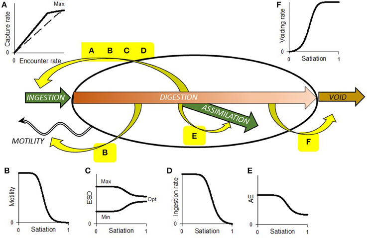
Figure 1. Schematic showing range of interactions between prey (food) encounter, ingestion, digestion, assimilation, and voiding. Yellow curved arrows indicate feedbacks; the sinusoidal arrow indicates consumer motility. Plot (A) shows the relationship between encounter and capture, which is initially linear but in the absence of any other feedbacks would be ultimately limited by handling at the point of capture or ingestion. The dashed line is for a prey type of lesser preference. Depending on preference, several prey items may be consumable over a period of time; consumption of any/all prey types contribute to satiation. Plot (B) shows satiation affecting motility, which in turn affects encounter rate (A). Set against this feedback is the need for some consumers to move for reasons other than feeding, and motion of the prey relative to the consumer caused by their own motility and/or turbulence. Plot (C) shows how prey preference, indicated here by size selectivity, may be expected to tighten as satiation develops. Plot (D) shows how gut satiation itself also controls ingestion rate, effectively decreasing the maximum level (plateau value) of capture indicated in plot (A). Plot (E) shows assimilation efficiency declining with satiation, so that in the presence of abundant food digestion is less complete. Plot (F) shows how, especially in a peristaltic gut, satiation promotes voiding. This works with (E), to counter (D) to enhance the flow through of food. The relationship between prey abundance (per unit of space) and ingestion rate is an emergent property of all these interactions, coupled to other facets such as food quality and prior nutritional history of the consumer.

The classic Holling type 2, or disk equation (Holling, 1965), is a widely used simple construct that describes “attack” and “handling” events in predator-prey interactions to generate a saturating (i.e., type 2) response curve. However, within plankton models, the most used function to describe this type 2 response is the rectangular hyperbola; from here on, we will reference this function as RHt2. RHt2 is often termed “Michaelis-Menten” or “Monod,” though these usages were originally for descriptions of enzyme-substrate kinetics or of microbial growth at limiting nutrient concentrations, respectively (Michaelis and Menten, 1913; Monod, 1949). Another type 2 function used for plankton grazing is the Ivlev function (Gentleman et al., 2003). The terms “Holling” and “type 2” are often synonymous in the plankton modeling literature, rather like “Droop” and “cell-quota model” for relating the internal resource availability to growth rate in phytoplankton (Flynn, 2008). In both instances naming conventions and citations are often inappropriate, clouding important differences between the original function and that actually deployed. The fundamental difference between the appearance of the disk function and RHt2 (and also Ivlev) is that the disk equation describes a linear (not a continuous curved) relationship between ingestion and prey abundance at low abundance. In contrast, Baird and Emsley (1999) describe grazing using a capped linear (i.e., type 1) function, as the minimum of a linear encounter rate and the maximum rate; there is no saturating term per-se.

The RHt2 function (Equation 1), as applied to predator-prey kinetics, describes ingestion rate [I; e.g., gC (gC)⁻¹ d⁻¹] through reference to constants defining the maximum ingestion rate [I_max; e.g., gC (gC)⁻¹ d⁻¹] and a half-saturation concentration of the prey (K_pred; e.g., gC m⁻³) with regard to prey availability (P; e.g., gC m⁻³). Saturation of the rate of ingestion at I_max may be ascribed to a limitation in “handling rate” (cf. Holling, 1965), though a precise physiological definition of this limiting factor is invariably lacking.

$\begin{array}{ll}I=I_{max}·\frac{P}{P+K_{pred}}& (1)\end{array}$

Changes in the form of the equation by raising parameter P to powers above 1 produce sigmoidal response curves (type 3); the form of such curves have been ascribed to events such as behavioral learning in higher animals (Holling, 1965; Real, 1979). To this base function (Equation 1) may also be included a threshold value of P below which predation does not occur; this is typically used to prevent prey extinction when P is low. Use of type 3 response curves (e.g., Ward et al., 2012) also minimizes the risk of extinction.

A commonly used (Gentleman et al., 2003) prey selectivity version of this RHt2 function (Fasham et al., 1990) is:

$\begin{array}{ll}{I}_i=I_{max}·\frac{p_i·P_i^2}{\left(\begin{array}{c}{K}_{pred}·\left(p_1·P_1+p_2·P_2+p_3·P_3+\dots \right)+\\ p_1·P_1^2+p_2·P_2^2+p_3·P_3^2+\dots \end{array}\right)}& (2)\end{array}$

Here, I_i is the ingestion rate on prey type i, present at abundance P_i, and consumed with relative preference p_i (such that Σp_i = 1). For applications to a single prey type (Equation 1), the units of operation may be individual- or biomass-based, but where multiple prey types are considered (Equation 2), the units are biomass-based. In Equation (2), prey type may be a species, closely allied groups of species, or more commonly a named functional type, such as “diatoms,” “flagellates” etc. The prey grazing function makes use of common I_max and K_pred values for all the different prey types. Other variants, such as the “kill-the-winner” prey-selection equation of Vallina et al. (2014), also make use of a single common half-saturation constant with units of external prey abundance. Cropp and Norbury (2009) make use of such reference to external prey abundance, although they use different K_pred values for alternate prey. Prowe et al. (2011) use a RHt2-like selection function but like many others refers to the RH terms as Holling type 2. Alternatively, in size-structured models, the selective grazing effort may be divided across the size spectrum of different prey sizes by reference to a log-normal predator:prey length ratio function (Ward et al., 2012).

The RHt2 function (Equation 1) is mathematically the same as the Monod relationships used to describe microbial nutrient-limited growth (Monod, 1949). For both applications (feeding and nutrient uptake), the equation describes an emergent consequence of a range of interactions, internal, and external to the organism. A common feature of both nutrient and prey acquisition in reality is satiation feedback. This feedback has been explored for nutrient acquisition by phytoplankton, and the implications for determining and modeling the kinetics of the event are understood (Flynn, 1998; Flynn et al., 1999). In contrast, few (e.g., Tirelli and Mayzaud, 2005; Mitra and Flynn, 2007; Thor and Wendt, 2010) have considered impacts of satiation feedback upon predation kinetics for planktonic consumers. Figures 1B–F shows the potential effects of satiation, which act over different time scales, on various aspects of predator-prey interactions, including processes of ingestion, digestion, assimilation and voiding of unconsumed material, predator motility, and prey (de)selectivity. Satiation is not described explicitly by the Holling disk equation (Whelan and Brown, 2005), though feedback may commence soon after acquisition of the resource (i.e., nutrient or prey), as the internal pool (vacuole or gut) fills. It is noteworthy that the RHt2 function only references the availability of external resources/prey, with no explicit inclusion of the important role played by satiation that results from the recent acquisition of all resources (Figure 1).

In this work, we identify several serious problems that arise from deployment of the widely used RHt2 function for the description of planktonic predator-prey interactions. Use of this function can readily yield results that are implausible when we consider the basis for real interactions. An important insight from our work is the realization that K_pred in the RHt2 equation (and other functions using K_pred-like terms), and especially when employed in multi-prey variants, represents a flawed concept which has scope for far over-estimating prey capture under the very conditions when capture would in reality be least likely. We present an alternative description that gives flexibility within realistic bounds, and does so at minimal computational cost for deployment in planktonic ecosystem models.

Background

Predator-prey ingestion interactions are complex and it is important to set the scene before progressing. The interactions may be broadly divided into two coupled components: (i) prey capture, including encounter rates with prey handling which may in turn include prey avoidance and/or rejection, and (ii) satiation feedback. Interactions between these components are indicated in Figure 1.

Prey Encounter and Capture

Descriptions of encounter kinetics for plankton have a well-established literature (Gerrittsen and Strickler, 1977; Rothschild and Osborn, 1988). There are several contributing factors which influence these kinetics; chief amongst these relate to predator and prey size, motion paths of both parties, and prey numeric abundance. The predator-prey size interaction defines the reactive distance, and may involve more than a simple collision between the prey and predator, especially where sight or olfaction is involved (e.g., Martel, 2006). Motility of the organisms may be considered as ballistic, or with some resemblance to Levy flight (Visser, 2008). The patterns of motion are suspected to affect fitness (Visser, 2007); unnecessary motility is potentially dangerous to the individual as it increases the likelihood of encountering a higher-trophic-level predator, as well as being energy sapping (Kiørboe, 2008). Motion paths of predator as well as prey can also be affected by factors such as nutritional status and turbulence. Thus, predator motility may decrease as satiation develops (Öpik and Flynn, 1989), or if turbulence is sufficient to aid predator-prey collision so enabling the predator to acquire prey through ambush rather than active hunting (Caparroy et al., 1998). Such factors also affect the way that the interactions may be modeled (Baird and Emsley, 1999; Pahlow and Prowe, 2010).

Experimental data over a range of zooplankton sizes demonstrate not only considerable variation in prey sizes for individual zooplanktonic predators, but also an enormous variation within the zooplankton functional group itself (e.g., protists vs. copepods vs. jellyfish; Mitra et al., 2014a). In general, feeding within the size spectrum may be expected to be greater against prey of larger size (Pahlow and Prowe, 2010). A composite of experimental data portraying the breadth of possible prey sizes for different zooplanktonic predators (Figure 2A), coupled with allometric relationships between plankton size and C-density (Figure 3), enables a consideration of the number of prey an individual predator needs to capture per minute (on average) to attain a C-specific ingestion rate of 1 d⁻¹ (Figure 2B). Such an ingestion rate would support a growth rate in the region of 0.15–0.3 d⁻¹ at typical values of gross growth efficiency (GGE; Hansen et al., 1997). The fastest particle ingestion rates thus calculated are in the order of a few 10's of items per minute; these are of prey of ca. <5% the linear size of the predator (e.g., ciliates ingesting bacteria, copepods eating small phytoplankton). Such prey are typically wafted in on currents as the predator continues to move rather than being subjected to raptorial “handling” as would befit the concept of mutually exclusive attack vs. handling events in the Holling disk equation. The larger the relative prey size and the slower the predator growth rate (decreasing the requirement rate for food), the lower is the required numeric ingestion rate (Figure 2B).

FIGURE 2

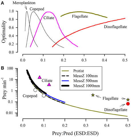
Figure 2. Relationships between relative size of predator and optimal prey size (A) and prey capture rates required to attain a given C-specific rate of ingestion (B). Panel (A) is redrawn from Hansen et al. (1994); the dinoflagellate plot peaks at a size ratio of 1:1. Panel (B) shows, as lines, the required continual capture rate per minute to attain a day average ingestion rate of 1 g prey-C (g predator-C)⁻¹ d⁻¹. These values were computed through reference to the allometric relationships for protists and mesozooplankton shown in Figure 3. Symbols show, as examples, maximum ingestion rates computed from relationships given in Hansen et al. (1997) for the organisms indicated.

FIGURE 3

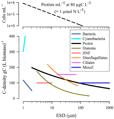
Figure 3. Relationship between equivalent spherical diameter (ESD) and C-density within the biomass. Data reconfigured from Straile (1997) and Menden-Deuer and Lessard (2000). The upper plot shows the number of protist cells of different size (using the “Protist” relationship from the lower plot) per mL of suspension when those organisms are present at a population biomass of 80 μgC L⁻¹, which equates to ~1 μmol biomass-N L⁻¹ assuming Redfield C:N for the prey. ESD provides a route to compare organisms of different volume with respect to a single linear dimension; implicit in this calculation is an assumption that the organism shape is not too different from a sphere, an assumption that becomes increasingly questionable for larger metazoan.

The range of estimates for maximum growth rates (μ), ingestion rates (I), GGE (= μ/I), and half-saturation constant (K_pred) for ingestion gained from experiments is very large (over an order of magnitude), and the allometric relationship in the raw data is non-significant (Hansen et al., 1997; Figure 4). It is not at all clear to what extent the great variability in these estimates is contributed to by the different nutritional states at the time of the studies of the predator, or indeed of the prey, or by other experimental issues (Karaköylü and Franks, 2011). Such matters are important, because prey ingestion kinetics for individual items have clear potential to vary according to the level of satiation caused by the cumulative ingestion of recently consumed prey (Figure 1; cf., Flynn (1998) for satiation control of nutrient transport into phytoplankton).

FIGURE 4

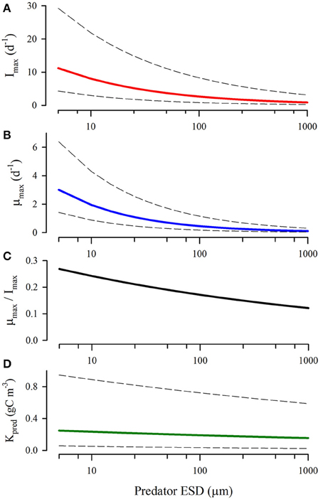
Figure 4. Relationships between predator size and maximum ingestion rate (A), growth rate (B), growth:ingestion rate [akin to GGE; (C)] and half-saturation value for prey (D). Redrawn from general relationships described in Hansen et al. (1997) showing mean (heavy lines) and values using standard errors (dashed lines).

Satiation Feedback

For most (likely all) consumers, the maximum ingestion rates attainable on typical feed must exceed the needs required to support the maximum growth rate by a considerable margin. If such an over-capacity in feeding potential was not present then the maximum growth rate could only ever be attained by feeding continuously in the presence of saturating prey abundance. That is patently not so, as consumers display discontinuous or moderated feeding behavior when supplied with food ab libitum in comparison with maximum rates observed following re-feeding of starved consumers. The value of I_max in the RHt2 equation (Equation 1) is in consequence most likely to be affected by gut (or, for a protist grazer, vacuole) satiation (Wirtz, 2013); limitation at “handling” is thus a limitation for handling the physiological processes of digestion etc. For planktonic grazers, limitation is unlikely to be at the stage of prey manipulations (i.e., raptorial handling) and is hence inconsistent with Holling disk equation terminology. The exception may be at prey sizes far below the optimum for that predator (Figure 2).

Satiation stems from the combined ingestion of all prey types over a period of time equating broadly to the gut (or feeding vacuole) transit time. Particles taken into a gut are unlikely to be completely consumed (assimilated); readily digestible material is recovered rapidly, and the remainder is ejected. In general, we expect the higher the ingestion rate, the fuller is the gut, and the lower is the assimilation efficiency (AE; Mitra and Flynn, 2007; Mitra et al., 2014a). Pahlow and Prowe (2010) explored optimal feeding behavior in zooplankton and showed the inverse relationship between ingestion rates and AE. There is thus potential for a series of interactions (Figure 1) that sees gut satiation controlling ingestion, yet also enhancing voiding, giving rise to the observed decline in gut transit time and in AE (Tirelli and Mayzaud, 2005). To all this, we add satiation feedback upon motility (Section Prey Encounter and Capture).

The problem, then, is how to resolve merging resource acquisition rates for different prey options, with changing values of maximum ingestion (varying as a function of collective food quality, perhaps, or with temperature), all in the support of a maximum growth rate, and using a computationally inexpensive function. For predator-prey interactions this translates to a need to be able to describe different rates of encounter, capture, and ingestion of individual prey items, with control (ultimately linked to maximum growth rate) to a common satiation level. To confront these challenges, below we describe the formulation of an alternative grazing function, through integration of a combination of the physiological processes governing grazing (Figure 1) and several well-established allometric functions that impact on prey capture and ingestion. We term this new function—the Satiation Controlled Encounter Based (SCEB) grazing function.

Materials and Methods

Developing an Alternative to RHt2

The Ingestion-Limited Selection (ILS) Grazing Function

We start with the ingestion-limited prey selectivity (ILS) function (Mitra and Flynn, 2006a) which we previously proposed as an alternative to the oft used Equation (2). The ILS function combines linear encounter terms for each prey type (akin to the “attack” component of the Holling disk equation) with a regulation of ingestion related to the total rate of biomass ingestion. Control of ingestion by “handling” is considered to occur from satiation feedback and the whole function thus combines explicit components of prey capture and satiation kinetics.

In the ILS function (Equations 3–5), Cp_i (Equation 3) is akin to the clearance rate, as defined in Hansen et al. (1997), with P_i (e.g., gC m⁻³) the biomass abundance of the ith prey type, and Cr_i (e.g., d⁻¹/(gC m⁻³)) the slope of the relationship between that prey's abundance and capture.

$\begin{array}{ll}C{p}_i=C{r}_i·P_i& (3)\end{array}$

The biomass-specific ingestion rate, I (Equation 4), is a minimum function of the total possible ingestion rate (sum Cp_i) and a curvilinear function that empirically describes a feedback on ingestion from satiation through reference to a half-saturation constant for the biomass ingestion rate of all prey items (K_I), and the maximum biomass-specific ingestion rate (I_max, d⁻¹).

$\begin{array}{ll}I=MIN\left(I_{\max }\cdot \frac{{\displaystyle \sum C{p}_i}}{\left({\displaystyle \sum C{p}_i+K_I}\right)},{\displaystyle \sum C{p}_i}\right)& (4)\end{array}$

Satiation feedback on ingestion is thus controlled by the half-saturation constant K_I, with higher values resulting in the feedback developing earlier. K_I is associated with the total ingestion rate and thence with satiation; it is not referenced to external prey abundance and hence there is no parameter in the ILS function equivalent to the K_pred term in RHt2 (Equation 1), and allied functions (e.g., Equation 2). The ingestion rate of the ith prey type is given as I_i (Equation 5).

$\begin{array}{ll}{I}_i=I·\frac{C{p}_i}{{\displaystyle \sum C{p}_i}}& (5)\end{array}$

To facilitate the implementation of the ILS function within ecosystem models that normally use RHt2, Cr_i and K_I can be set from values of I_max and K_pred via Equation (6) (e.g., Mitra and Flynn, 2006a; Sailley et al., 2015).

$\begin{array}{ll}{K}_I/C{r}_i\equiv K_{pred},C{r}_i\equiv \frac{I_{max}}{4·K_{pred}},\mathrm{\text{and thus }}{K}_I\equiv I_{max}/4& (6)\end{array}$

It must be stressed that there is no reason to set K_I as a function of I_max at all; doing so (Equation 6) merely provides a route to match the upper (plateau) section of the ILS and RHt2 curves to aid comparisons.

Formulating the Satiation Controlled Encounter Based (SCEB) Grazing Function

In this section we explicitly define the dynamics of particle-particle (prey-predator) encounter to derive biologically justifiable values for Cp_i (Equation 3) for placement in the ILS equations. This is achieved by incorporating facets of several well-established allometric functions that describe encounter rates with reference to motion paths, and biomass-specific ingestion rate transforms. Like most applications of allometric-related facets of plankton ecophysiology, we refer to plankton organism size by reference to an assumed equivalent spherical diameter, ESD. Encounter is assumed to be a function of collision between organisms of stated ESDs.

The encounter rate by a predator (Enc_s, prey predator⁻¹ s⁻¹) is described by Rothschild and Osborn (1988) as:

$\begin{array}{l}En{c}_s=\pi {(r_a+r_z)}^2·N·(C_a^2+3·C_z^2+4·w^2)\\ ·{(C_z^2+w^2)}^{-0.5}·3^{-1}& (7)\end{array}$

Here, the subscript a identifies the less motile of the organisms (usually the prey), subscript z the more motile organism (usually the predator), r is the organism radius (m), C is their speed of motion (m s⁻¹), w is root-mean-squared turbulence (m s⁻¹), and N is numeric prey abundance (items m⁻³).

Motion of plankton occurs through a combination of their own motility and also of turbulence. By default we assume ballistic paths for those organisms that are motile, as these serve, assuming homogeneous distribution of prey, to maximize encounters. The data summarized in Figure 5 gives a relationship between organism size (ESD, data values ranging between 1.2 and 1900 μm) and motility (C, m s⁻¹) as described in Equation (8).

$\begin{array}{ll}C=10^{-6}·(38.542·ES{D}^{0.5424})& (8)\end{array}$

FIGURE 5

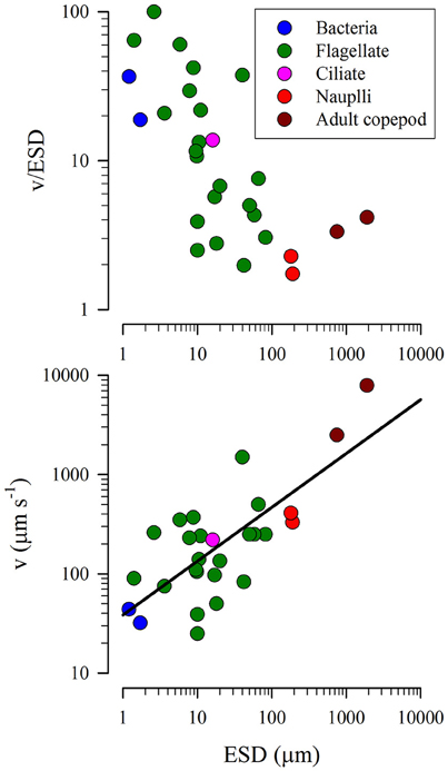
Figure 5. Relationship between equivalent spherical diameter (ESD) and speed of motion (v). Data from Sommer (1988) and Visser and Kiørboe (2006). The line in the lower plot has the equation, C = (38.542 · ESD^0.5424).

Rothschild and Osborn (1988) provide a relationship between wind speed and root-mean squared turbulence (w in Equation 7). They considered values of w from 0 to 0.003 m s⁻¹, noting the relative importance of turbulence for encounters with smaller organisms.

Encounter rate per day (i.e., prey predator⁻¹ d⁻¹) is thus:

$\begin{array}{ll}En{c}_d=En{c}_s·60·60·24& (9)\end{array}$

Next the C-biomasses of prey and predator organisms are required; these are assumed to accord to allometric functions of their ESDs. The data presented in Figure 3, show a preponderance of biomass densities around 200 gC L⁻¹.

The form of the relationship used here is:

$\begin{array}{ll}orgC=\frac{a}{1000}·{\left({\left(\frac{4}{3}\cdot \pi \cdot \frac{ESD}{2}\right)}^3\right)}^b& (10)\end{array}$

Organism C-biomass (orgC; ngC individual⁻¹) is computed for both prey C and pred C by reference to their ESD (μm). For a protist, the values of a and b used were 0.216 and 0.939, respectively; for a mesozooplankton these values were 0.1 and 1 (Menden-Deuer and Lessard, 2000).

The C-biomass specific ingestion rate (prey-C predator-C⁻¹ d⁻¹ = d⁻¹), assuming encountered prey are actually ingested, is then given by:

$\begin{array}{ll}C{p}_i=En{c}_d·\frac{preyorgC}{predorgC}& (11)\end{array}$

Cp_i, as computed through Equation (11), is now a direct input for the ILS function and replaces the original definition given in Equation (3).

In total, the SCEB grazing function is defined by combining the Equations (7–11) with those describing ILS (i.e., Equations 4, 5). SCEB thus provides a description of predator-prey ingestion kinetics potentially attainable in reality through reference to predator and prey sizes, motilities, and prey abundance. An additional advantage of using SCEB, instead of the previously described ILS, is the capability of describing ingestion in terms of individuals as well as biomass.

Comparisons between RHt2 and SCEB Functions

We compare the predator-prey kinetics described using a conventional biomass-based RHt2 function against the SCEB grazing function making use of two indices.

(i) We compare the value of the half-saturation constant for predation, K_pred (gC m⁻³), used within RHt2 against the value of prey concentration that enables half I_max using SCEB; this latter value is referred to as K_0.5, to differentiate it from K_pred. It should be noted that K_0.5 is an emergent feature of SCEB calculated to aid comparisons against K_pred; it should not be confused with K_I (see text for Equation 4).

(ii) Ingestion rates computed from SCEB (hereafter I^SCEB), according to the encounter rate descriptions given in Equations (7–11), are deemed to be at the upper range of biologically plausible. The ratio between I from RHt2 (hereafter I^RH) and I^SCEB, for a given prey abundance thus gives an indication of the plausibility of the grazing described by I^RH. Values of I^RH/I^SCEB >1 are deemed implausible as the encounter rates defined by the allometric relationships for biomass-specific encounters and motility (coupled, as appropriate, with turbulence fields), could not occur even when assuming ballistic motion paths. In contrast, values of I^RH/I^SCEB < 1 are attainable through modifications to behavior (e.g., swimming speed or prey selectivity) and/or satiation linked regulation of ingestion (achieved empirically here by altering the value of K_I in Equation 4).

Comparisons between Performance of Selectivity Functions Using RHt2 and SCEB

We present a comparison between the usage of RHt2 prey selectivity function (Equation 2) and a selectivity-function variant of SCEB, as applied to the experimental data of Flynn et al. (1996). The model used for this work described a multi-element based structure, with variable C:N stoichiometry for the prey, and is developed from that we have described before (Mitra and Flynn, 2006a). The only change was that the prey encounter description used in the original paper (Equation 3) was replaced with SCEB (using Equations 7–11). Construction and simulation of models were carried out using Powersim Constructor v2.51 (Isdalstø, Norway), as in Mitra and Flynn (2006a). Optimizations (tuning) of model to the experimental data describing predator selection and de-selection between three prey of different sizes, were obtained using Powersim Solver v2. This tuning software uses an evolutionary (“genetic”) algorithm that operates by running the model many 100's of times with different combinations of parameter values for the predation terms. Ultimately the combination of parameter values that minimizes differences between model output and experimentally-derived values are identified.

Results

Figure 6 shows a comparison between the potential grazing rates as computed using the SCEB function vs. the RHt2 comparator; these make use of the indices (i) and (ii) described in Section Comparisons between RHt2 and SCEB Functions. The initial slopes for all the RHt2 curves significantly exceed that described by SCEB (Figure 6A). RHt2 thus returns grazing rates that become increasingly implausible at lower prey concentrations (I^RH: I^SCEB >1; Figure 6B). The use of high K_pred values in the RHt2 description, while returning more plausible grazing rates at low prey concentrations (i.e., curves closer to the SCEB description in Figure 6A), at high prey abundance give grazing rates that are much lower, such that I_max could only be achieved at very high prey abundance levels.

FIGURE 6

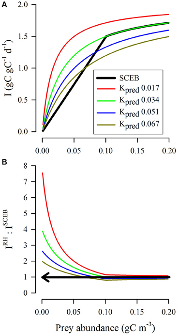
Figure 6. Comparison between outputs from RHt2 and SCEB functions relating prey availability to grazing rate under conditions of zero turbulence for a protist grazer of 20 μm ESD feeding on a protist prey of 4 μm ESD. In all instances, I_max = 2 d⁻¹, sufficient to support a predator biomass doubling per day (0.693 d⁻¹) at typical gross growth efficiencies (Hansen et al., 1997; Straile, 1997). The SCEB function curve is computed using the allometric relationships for both biomass and motility (both prey and predator assumed to be motile), with no turbulence, and with K_I set as equivalent to I_max/4 (Equation 6) to aid comparisons with RHt2. The RHt2 curves are computed using various values of K_pred, one of which (0.034 gC m⁻³, equating to 0.42 μmol biomass-N L⁻¹ at Redfield C:N) matches the SCEB output most closely. (A) For RHt2 functions, the half-saturation constant K_pred was set at the value indicated (gC m⁻³). The SCEB function (black line) matched that of the RHt2 output with K_pred = 0.034 gC m⁻³ (green line). (B) Ratio of the RHt2 to SCEB (I^RH: I^SCEB) outputs. Values of I^RH:I^SCEB above 1 (indicated by the arrow) are implausible as encounter rates cannot support such grazing rates, as per the allometric scalars used for the SCEB function.

Figure 7 gives an extension of the analysis shown in Figure 6A, now with the inclusion of turbulence. For SCEB this invokes the turbulence term in Equation (7); the RHt2 function has no capacity for explicit reference to turbulence. The closest comparisons between RHt2 and the SCEB descriptions are given when low K_pred values are used in RHt2 and also a high turbulence value is assumed for the SCEB calculations. Plausibility of the RHt2 description (i.e., I^RH: I^SCEB ≤1) is thus improved in applications to highly turbulent systems; here encounter rates are strongly affected by abiotic events and allometric interactions are of less importance.

FIGURE 7

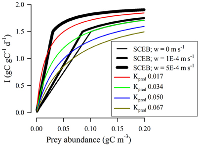
Figure 7. Comparison between outputs from RHt2 and SCEB functions relating prey availability to grazing rate under different conditions of turbulence for a protist grazer of 20 μm ESD feeding on a protist prey of 4 μm ESD. In all instances, I_max = 2 d⁻¹. For RHt2 functions the half-saturation constant K_pred was set at the value indicated (gC m⁻³). The black lines show outputs of the SCEB function when operated under different levels of turbulence, as indicated. Under conditions of zero turbulence (root-mean squared, w = 0 m/s) the SCEB function matched that of RHt2 with K_pred = 0.034 gC m⁻³.

Half-saturating prey concentrations (values of K_0.5) defined by SCEB range over an order of magnitude (Figure 8A); they are higher for ingestion of relatively smaller prey, and are also higher for larger predators. For reference, a K_0.5 of 0.2 gC m⁻³ (which is broadly mid-range of the experimentally derived estimates of K_pred, Figure 4D), equates to ≈2.5 μmol biomass-N L⁻¹ assuming Redfield C:N. The kinetics described in Figure 8A assume zero turbulence. As turbulence is increased then encounter rates also increase, and hence the effective half-saturation constant (K_0.5) decreases. However, the rate in decrease of K_0.5 varies with the size of the predator and the relative size of its prey. This is shown in Figure 8B, with a value above 1 indicating a pro rata increase in potential grazing rates when grazing in turbulent conditions due to the decrease in K_0.5. For smaller grazers (Figure 8B), the effect of turbulence provides scope for a decrease in K_0.5 by an order of magnitude (i.e., encounter rates increase 10-fold in the presence of turbulence). In contrast, the changes in the value of K_0.5 with turbulence are relatively low for the largest predator considered (ESD = 1 mm). The increased plausibility of the RHt2 description in applications at high turbulence levels (i.e., I^RH: I^SCEB ≤1; Figures 6, 7) thus only holds for descriptions of the activity of smaller (protist) predators, and not for larger predators such as adult copepods.

FIGURE 8

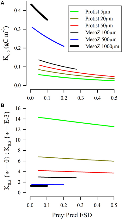
Figure 8. Biomass-specific concentrations of prey required to half saturate grazing (K_0.5) as derived from the SCEB function for predators configured as either protist or mesozooplankton, and of different size (ESD, as indicated). Both prey and predator were considered as motile, and I_max = 2 d⁻¹. (A) Relationship between the ratio of prey:predator size and K_0.5 under conditions of zero turbulence (i.e., root-mean squared, w = 0 m s⁻¹). (B) Relative values of K_0.5 for turbulent (w = 1E-3 m s⁻¹) vs. non-turbulent (w = 0 m s⁻¹) conditions.

Another way of viewing the interactions of predator size, relative prey size and turbulence (in addition to the effect on K_0.5 as shown in Figure 8) is to consider the effect of these parameters on the value of the encounter rate. The slope of the encounter rate, Cr_i, defines the relationship between prey availability and capture potential (see Equation 3). Figure 9 shows the biomass-specific values of Cr_i for different combinations of predator types, different prey:predator sizes, and ± turbulence. The higher the value of Cr_i, the faster the potential grazing rate, and the lower is K_0.5 for a given I_max. There is an order of magnitude difference in potential grazing rates across the spectrum of zooplankton sizes, increasing to two orders of magnitude when turbulence is included.

FIGURE 9

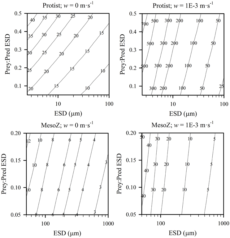
Figure 9. Contour plots of predator size (ESD) against relative size of prey in terms of ESD (Prey:Pred), shown for protist and mesozooplankton predators, in non-turbulent (root-mean squared, w = 0 m·s⁻¹) and turbulent (root mean squared, w = 1E-3 m·s⁻¹) conditions, the slope of the encounter rate, Cr_i ((gC gC⁻¹ d⁻¹)·(gC prey m⁻³)⁻¹). All prey were considered as protists, and both predator and prey were considered motile. Outputs are generated from the allometric scaling rules in the SCEB function.

Figures 10, 11, for microzooplankton and mesozooplankton, respectively, show great variation in the emergent half-saturation (K_0.5) values, across a range of values of I_max and prey size, with different levels of turbulence. Only for larger non-ambush mesozooplankton predators (i.e., excluding non-motile predators) does the prey size not significantly affect K_0.5 (Figure 11C).

FIGURE 10

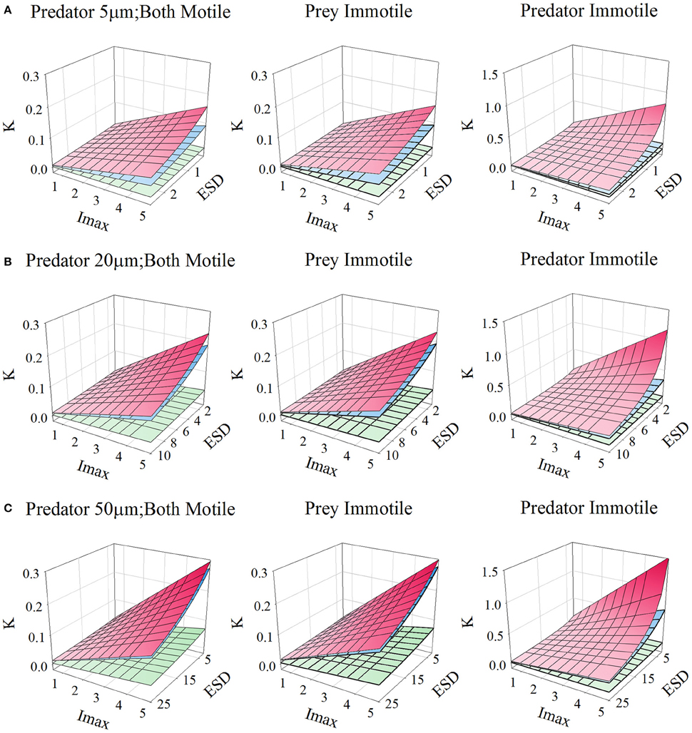
Figure 10. Relationship for protists of different sizes [panels (A–C)], between prey size (ESD, μm), maximum grazing rate (I_max, C C⁻¹ d⁻¹), and the prey biomass concentration required to support I_max/2 (K, gC m⁻³; for reference, 0.1 gC m⁻³ ≡ 1.26 μmol biomass-N L⁻¹ assuming a Redfield C:N). Plots show the relationships when both predator and prey are motile, or when only one or the other is motile. In each plot the upper plane (red gradient) assume a root-mean squared turbulence (w) of 0 m s⁻¹, middle plane (blue gradient) of 1E-4 m s⁻¹, and the lower plane (green gradient) of 1E-3 m s⁻¹; the upper and middle planes are very close to each other in many instances. Outputs are generated from the allometric scaling in the SCEB function.

FIGURE 11

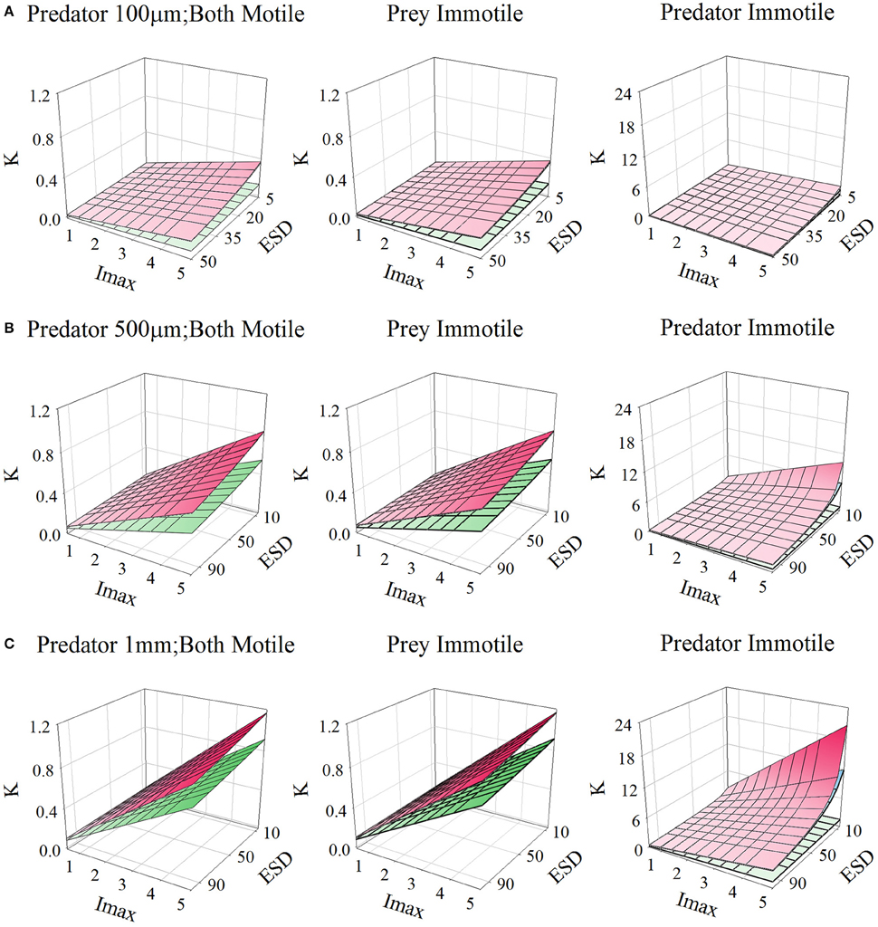
Figure 11. Relationship for mesozooplankton of different sizes [panels (A–C)], between prey size (ESD, μm), maximum grazing rate (I_max, C C⁻¹ d⁻¹), and the prey biomass concentration required to support I_max/2 (K, gC m⁻³; for reference, 0.1 gC m⁻³ ≡ 1.26 μmol biomass-N L⁻¹ assuming a Redfield C:N). Plots show the relationships when both predator and prey are motile, or when only one or the other is motile. In each plot the upper plane (red gradient) assume a root-mean squared turbulence (w) of 0 m s⁻¹, middle plane (blue gradient) of 1E-4 m s⁻¹, and the lower plane (green gradient) of 1E-3 m s⁻¹; the upper and middle planes are very close to each other in many instances. Outputs are generated from the allometric scaling in the SCEB function.

Figure 12 presents a comparison of model fits to experimental data when the different grazing functions (i.e., RHt2 vs. SCEB) were used. The experimental data, from Flynn et al. (1996), are for the protist Oxyrrhis (ESD 16–20 μm) feeding on three alternate motile prey of different size—the protists Micromonas (ESD 1.5 μm), Isochrysis (ESD 4.5 μm), and Dunaliella (ESD 7.6 μm). The data show a changing pattern of prey selectivity expressed by the predator according to the nutrient status of the prey as well as prey size (the predator working its way from larger to smaller prey). The experimental system is complex, with the value of Cr_i for the smallest prey (Micromonas; Cr_Micomonas) being zero when alternative palatable larger prey are available. For Isochrysis, Cr_Isochrysis decreases as the quality of this prey item becomes lower due to nutrient limitation (this is related to the Isochrysis N:C; see Mitra and Flynn, 2006a). For each fit (RHt2 or SCEB) a genetic (evolutionary) algorithm was used to optimize the match of the model to the data; see Section Comparisons between Performance of Selectivity Functions Using RHt2 and SCEB. Figure 12A demonstrates the inability of the RHt2 ratio-based approach (Equation 2) to match the experimental data. In this particular system, the predator shows near-ballistic motion paths only when starved; Oxyrrhis motility slows significantly as it becomes satiated (Öpik and Flynn, 1989). Further, the prey flagellates used in these experiments actually swim very slowly in small circles; their motion certainly could not be described as ballistic. Setting the prey motion to zero, and then allowing the model to tune the swimming speed of the predator gives a good fit when the predator is assumed to have an average swimming speed of <20% of the allometric-scaled ballistic rate (Figure 12B).

FIGURE 12

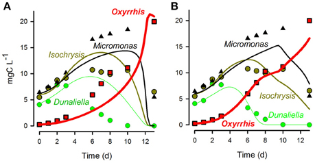
Figure 12. Fits (lines) of alternative descriptions of selective predation to data (symbols) for the protist Oxyrrhis growing through predation upon the phyto-flagellates Dunaliella, Isochrysis, and Micromonas (data from Flynn et al., 1996). (A) Fit of the RHt2 ratio-based function Equation (2). (B) Fit of the SCEB function assuming no motion of the prey, and the predator speed set at 20% of the SCEB-derived value. See text for further comment.

Discussion

Apparent Dysfunctionality in RHt2

The most widely used function describing predator-prey interactions in planktonic ecosystem models is the RHt2 equation (Equation 1) or a variant of it. This RHt2 equation forms the core of the zooplanktonic predator-prey descriptions in the ocean carbon cycle components of CMIP5 Earth System Models (Arora et al., 2013; Bopp et al., 2013) as well as having a long historic pedigree (e.g., Fasham, 1995; Gentleman et al., 2003; Blackford et al., 2004; Plagányi, 2007; Anderson et al., 2010). However, as we have shown here, there are serious problems associated with using the RHt2 function. Below are listed the major conclusions from the work described here relating to deployment of RHt2 equations:

(i) RHt2 equations readily describe planktonic predation kinetics that, on the face of it, appear implausible, a situation that becomes increasingly likely at lower prey concentrations, and for non-turbulent conditions (Figures 6, 7).

(ii) The use of the RHt2 functional response for the description of predator-prey feeding kinetics for a given predator consuming a range of prey sizes, using the same single biomass abundance-specific K_pred value (Equation 2) for all prey types irrespective of their abundance, size, and motility appears flawed. It is implausible that acquisition of such prey could possibly share such kinetics, except perhaps for larger mesozooplankton; differences in prey size have profound effects on encounter rates and on half-saturation values (K_0.5 in Figures 8, 10, 11).

(iii) The use of RHt2 to describe predation kinetics for a single functional group containing predators of significantly different sizes (e.g., micro- to meso-zooplankton) using a single set of kinetic parameters, appears flawed; it is biologically implausible that feeding kinetics could possibly share common values (Figures 8–11).

(iv) RHt2 descriptions cannot correctly describe selection between different prey items, and are also not capable of describing the de-selection of individual prey types (Figure 12A). Indeed, prey preference derivatives of the RHt2 function (Equation 2) appear fundamentally flawed (Mitra and Flynn, 2006a).

(v) RHt2 descriptions offer no scope for inclusion of turbulence that profoundly affects plankton encounter rates (Figures 8–11).

The rectangular hyperbolic shape of RHt2 presents a core problem. In order to prevent implausible rates of grazing at low prey availability, K_pred needs to be so high that the overall form of the RHt2 function then becomes too shallow at higher levels of prey abundance (Figure 6). Only if one assumed protist predators in highly turbulent waters do the curves described by RHt2 start to align with those projected to be plausible by SCEB (Figure 7). The excessive grazing rates described by the RHt2 function at the lowest prey concentrations results in the simulated grazer being furnished with too many prey, stimulating excessive grazer growth and nutrient regeneration, and raising the risk of prey extinction in the model. In ecosystems where poor prey quality adversely affects predator-prey interactions (Hessen et al., 2002; Mitra and Flynn, 2005, 2006b; Polimene et al., 2015) it is particularly important to describe the dynamics of these interactions correctly as they can lead to the formation of ecosystem disruptive algal blooms (EDABs) that block trophic transfer (Mitra and Flynn, 2006b). A traditional solution to the problem of over-predation at low prey abundance is to deploy a threshold control, or to use a sigmoidal (type 3) function (Gentleman et al., 2003; Ward et al., 2012; Cordoleani et al., 2013; cf. Morozov, 2010). However, such short-cut solutions add additional parameters with no clear mechanistic justification. An additional problem relating to the continuous curve form of RHt2 is that it is not possible to independently alter the initial kinetics of predation and also the maximum ingestion rate. Thus, increasing I_max, for example in response to elevated temperatures, also simultaneously increase the apparent rates of encounter. Given that there is no temperature term in the motility equation, Equation (8; see legend to Figure 5), such a direct relationship seems unlikely.

The logical consequence of the above is that RHt2 descriptions are ill suited for describing planktonic predation kinetics, and that we should seek to replace them. We propose that SCEB offers a suitable replacement. Below we discuss some of the features of SCEB that we suggest make it attractive in this regard.

SCEB vs. Holling Disk Equation

The classic, archetypal description of predator-prey kinetics is the Holling type 2 disk equation (Holling, 1965). As mentioned in the Introduction, RHt2 terms are often (mis)labeled as Holling type 2, even though the equations have nothing in common. In contrast, SCEB shares various common features with the disk equation. While RHt2 and Ivlev response functions describe continuous curves, the SCEB response curve is similar to the disk equation, with its initial linear attack (encounter) rate, followed by a saturating phase. However, the actual implementation and mechanistic justification for the equations are different in several important ways. Firstly, the disk equation assumes that attack and handling are mutually exclusive, and furthermore not only do attack rates vary between prey types (as they do in SCEB) but so do the handling times. The disk equation has its origins for applications (terrestrial animals) where the processes of prey handling interferes directly with attack upon the next prey item. Accordingly, the disk equation typically uses pairs of attack and handling parameters for each prey type thus significantly increasing parameterization effort. For most planktonic grazers either prey are wafted in rapidly while the zooplankter swims, or the prey is so large and yet engulfed with such speed (relative to the number of events needed per day) that handling limitation operates predominantly via satiation (Wirtz, 2013). In SCEB that handling interaction (for one to multi-prey) has one handling parameter which is linked to the total biomass ingested over the recent past, thus making the link to satiation.

Application of the disk equation alone for deployment in planktonic ecosystem models is insufficient. Ultimately in reality, and also in the arena in which these descriptions are used for planktonic predator-prey interactions, the value of the rate described by the plateau of the prey abundance-ingestion response curve (I_max) is pivotal to the behavior of these models (Mitra et al., 2014a); the disk equation does not include such a value. The maximum value of ingestion derived from the disk equation is an interactive term between attack and handling at the point of ingestion only and the plateau value thus varies for every combination of attack rate and handling time. Whelan and Brown (2005) indicate the value of coupling a satiation linkage to the disk equation, but this then adds another level of computation.

In summary, the SCEB function uses meaningful attack rates (same as the disk equation), with a single (satiation-linked) handling-rate control, and a meaningful maximum ingestion rate. Compared to SCEB, the disk equation requires potentially double the number of constants (each prey item needing both attack and handling constants), plus an additional satiation term.

Advantages and Benefits of Using the SCEB Function

The ILS function was originally proposed as an alternative to RHt2 for representation of multiple prey-predator interactions, especially for prey switching situations (Mitra and Flynn, 2006a; Mitra et al., 2007). SCEB is an enhanced description of the ILS function which provides an extended, explicitly allometric, basis upon which to model plankton predator-prey interactions. Here, we consider some additional facets of using SCEB that are applicable for ecosystem scale models that require computationally efficient solutions.

Motility and turbulence have important implications for planktonic predator-prey interactions (Saiz et al., 1992; Thomas and Gibson, 1992; Caparroy et al., 1998; Dolan et al., 2003). The allometric-scaling of the consequence of turbulence for predator-prey interactions has also long been recognized (Rothschild and Osborn, 1988; Kiørboe, 1993; Baird and Emsley, 1999). Exploration of the coupled allometric and biomass-specific consequences on grazing becomes particularly apparent through usage of the SCEB function (Figures 7–11). The RHt2 function, in comparison, has no scope to describe any of these important interactions, to independently alter the slope of encounter and capture of prey of different size and motilities.

In situations where prey are limiting, it may be assumed that ballistic paths are appropriate; thus the SCEB formulation describes correctly the experimentally observed bacteria ingestion by heterotrophic nanoflagellates and mixotrophs reported by Zubkov and colleagues for oligotrophic waters (e.g., Hartmann et al., 2012). In other situations, however, feedback control by satiation is expected to down-regulate the potential for grazing. Satiation is expected to affect motility (decreasing encounter rates with prey, but also having the benefit of decreasing encounter rates with higher trophic level predators) and also capture rates (decreasing ingestion rates even where encounters occur). SCEB provides a framework for the exploration of satiation-linked processes (and other factors) that affect grazer motility which then affects predation pressures exerted by the next trophic level. To enable a fit of SCEB to experimental data (Figure 12B) we had to assume much lower swimming speeds that ballistic motion paths would define; this requirement is entirely consistent with empirical evidence of the behavior of the satiated grazer (Öpik and Flynn, 1989). An extension of such a framework can also be used for the allocation of different grazing kinetics across predators, and upon prey, of different size and activity. The SCEB function can thus help to better delimit predator-prey kinetics (noting the wide range of experimental data—Hansen et al., 1997; Figure 4), removing reliance upon the tuning-based allocation of K_pred values in RHt2-style functions as applied in ecosystem models.

Feedback attributed to satiation in the ILS and SCEB functions is identified as stemming from nutritional satiation; hence the involvement of the total acquired food biomass in the control term for I_max and K_I (Equation 4). However, it is possible that for some predator-prey combinations satiation could occur at the point of prey handling during capture and ingestion. While it would seem unlikely that a predator-prey relationship would evolve in which handling of optimal prey in the natural environment restricts the day averaged ingestion rate, there are instances where that may occur; these include the presence of interfering materials such as mucus or silt particles. The SCEB description could handle such a situation by introducing an interference term on all Cp_i values as a function of the abundance of the interfering substance. Such a control would be similar to the de-selection terms described and deployed by Mitra and Flynn (2006a,b), that down-regulate the potential Cp_i values according to prey quality.

Finally, with SCEB, as it is possible to separate the kinetics controlling satiation (with I_max) from that affecting encounter rates, introducing temperature does not automatically affect both of these features as is the case with RHt2. SCEB thus seems a more appropriate platform than RHt2 for considering impacts of environmental change that affect changes in consumer metabolism.

Predator-Prey Kinetics for Functional Type Descriptions within Food-Web Models

In a classic NPZ type of model (e.g., Fasham et al., 1990; Fasham, 1995), a single value of K_pred is used to describe the half-saturation constant for all prey types into a single zooplankton box intended to account for the activity of all zooplankton types and sizes. Even in extant widely used ecosystem models only a few zooplankton functional types are included, coupled to a similar number of prey options (Arora et al., 2013; Bopp et al., 2013), or sometimes to very many phytoplanktonic prey types (e.g., Vallina et al., 2014). Thus, within these models, a wide range of zooplankton sizes and thence potential prey preferences (Figure 2A) are amalgamated together. The values of K_0.5 shown in Figure 8A are much greater than RHt2 K_pred values of 1 μmol biomass-N L⁻¹ used in applications by Fasham (1995), of 0.040–0.045 gC m⁻³ used by Blackford et al. (2004), and of 0.012–0.036 gC m⁻³ used by Anderson et al. (2010). Such models not only use the same half-saturation constants to describe interactions over a wide predator and prey range, but they also use a similar restricted set of maximum ingestion (or growth) rates. These descriptions also do not appear to likely accord with biologically realistic behavior. SCEB outputs (Figures 8A, 10, 11) indicate scope for a range of K_0.5 over an order of magnitude for such combinations, depending on the size of prey and predator and also of motility, with or without turbulence. It is also noteworthy that the values of K_0.5 generated with SCEB fall closer to the central region of the data collated by Hansen et al. (1994; Figure 4D).

The results from our analysis shows the significant scope for allometric and growth rate scaling through systems of different chemico-physical characteristics, affecting biomass abundance through nutrient availability, and turbulence. There are wide differences in K_0.5 for larger vs. smaller zooplankton (Figures 8, 10, 11). High growth rates of larger predators are thus only sustainable at high prey abundance loadings; these are to be expected to be allied to high nutrient loadings and this assumes that their AE are similar, while more likely AEs are lower in mesozooplankton (Mitra et al., 2014a). This situation is expected to extend through to higher trophic levels due to inefficiencies in trophic transfers. Microbial-scale grazers are likely favored at low nutrient loadings (i.e., they have significantly lower K_0.5; Figures 8A, 10 vs. Figure 11) as a consequence not only of basic allometric relationships but also because protist grazers consume relatively much larger prey (Figure 2A). While it is apparent that consumption of bacteria-sized prey can only support rapid growth of small grazers, the application of the SCEB equations to models of mixotrophic protists (these organisms now being acknowledged as important components of oligotrophic oceans; Hartmann et al., 2012; Mitra et al., 2014b, 2016) will help indicate conditions under which phototrophy or phagotrophy may be expected to be more or less important.

The use of much lower K_pred values in ecosystem models than appear plausible from our analysis could be taken (or argued to be justified) as—(i) a reflection of the implicit importance of smaller grazers (which have a lower K_0.5; Figure 8A), and/or, (ii) that bulk measurements (i.e., mean field densities; see Grünbaum, 2012) are significantly underestimating prey density fields as experienced by the grazers in reality. However, the use of K_pred values across such wide ranges of predator and prey, coupled with the emergent properties (excessive grazing) of RHt2 at low prey abundance, could be equally argued to be masking structural problems in the conceptual basis of the model. Deployment of SCEB forces the modeler to consider the allometric and growth rate implications of reality, while providing scope for enhanced model fidelity in biological and abiotic capacities.

There is, however, the challenge of how we should parameterize models that do indeed group together functional types that span wide size ranges. Our analysis suggests that applying single sets of parameters is liable to generate implausible descriptions of reality. This problem is acute for RHt2, but the issues identified in (ii) and (iii) in Section Apparent Dysfunctionality in RHt2 also apply to deployment of any description of predator-prey interaction. The options here would appear to be to either split those functional groups up (are predators of such different size really part of the same ecologically-consequential functional group? See Mitra et al., 2014a, 2016; Flynn et al., 2015) or to assume that pragmatically the bulk of the activity is associated with organisms of a particular size and configure SCEB accordingly. There are other reasons to at least differentiate between protist and metazoan grazers, as not only is there often a profound difference in relative prey size (Figure 2A; Hansen et al., 1994) but the mechanics and kinetics of events differ greatly (Tirelli and Mayzaud, 2005; Flynn, 2009; Pahlow and Prowe, 2010; Montagnes and Fenton, 2012).

Conclusions

While there are many caveats for deploying any allometric-scaled equations to describe complex behavioral and ecological processes, SCEB, has clear advantages over RHt2, its multi-prey derivations, and other functions that make reference to half-saturation constants with units of external prey abundance. While SCEB has similarities, and hence common mechanistic grounds, with the classic Holling type 2 disk equation, the use of a single handling constant (here labeled for “satiation”) and a defined maximum ingestion rate makes SCEB more attractive for deployment in planktonic ecosystem models. In addition to providing solutions to the challenges associated with deployment of RHt2, the simplicity of the SCEB function offers potential for:

(a) An extended theoretical consideration of predator-prey interactions, including explorations of activity in patches, and the challenges of mean-field computations of predation dynamics (Grünbaum, 2012).

(b) A role as a front-end to more complex models considering multiple prey types of different quality and quantity, together with satiation and variable assimilation efficiency, and changes in predator size and motility with developmental stage.

With no significant additional computational cost, the SCEB function overcomes all the shortcomings of the RHt2 function (and allies) and provides a direct route to involving physics, changes in predator and/or prey size and motility, and prey palatability (thus allowing true de-selection of prey types). SCEB can also be directly incorporated within individual-based as well as biomass-based models. Importantly, SCEB requires (enforces) an acknowledgement of allometrics in biomass-based models, which typically make scant reference to size even when (as for predator-prey interactions, as we have seen) it is necessary to do so.

Author Contributions

AM and KF equally contributed to all aspects of this work.

Conflict of Interest Statement

The authors declare that the research was conducted in the absence of any commercial or financial relationships that could be construed as a potential conflict of interest.

Acknowledgments

This work was funded by the Natural Environment Research Council (NERC, UK) through its iMARNET programme NE/K001345/1. We are indebted to referees of an earlier version of this work.

References

Anderson, T. R., Gentleman, W. C., and Sinha, B. (2010). Influence of grazing formulations on the emergent properties of a complex ecosystem model in a global ocean general circulation model. Prog. Oceanogr. 87, 201–213. doi: 10.1016/j.pocean.2010.06.003

CrossRef Full Text | Google Scholar

Arora, V. K., Boer, G. J., Friedlingstein, P., Eby, M., Jones, C. D., Christian, J. R., et al. (2013). Carbon–concentration and carbon–climate feedbacks in CMIP5 earth system models. J. Climate 26, 5289–5313. doi: 10.1175/JCLI-D-12-00494.1

CrossRef Full Text | Google Scholar

Baird, M. E., and Emsley, S. M. (1999). Towards a mechanistic model of plankton population dynamics. J. Plankt. Res. 21, 85–126. doi: 10.1093/plankt/21.1.85

CrossRef Full Text | Google Scholar

Blackford, J. C., Allen, J. I., and Gilbert, F. J. (2004). Ecosystem dynamics at six contrasting sites: a generic modelling study. J. Mar. Sys. 52, 191–215. doi: 10.1016/j.jmarsys.2004.02.004

CrossRef Full Text | Google Scholar

Bopp, L., Resplandy, L., Orr, J. C., Doney, S. C., Dunne, J. P., Gehlen, M., et al. (2013). Multiple stressors of ocean ecosystems in the 21st century: projections with CMIP5 models. Biogeosci. 10, 6225–6245. doi: 10.5194/bg-10-6225-2013

CrossRef Full Text | Google Scholar

Caparroy, P., Pérez, M. T., and Carlotti, F. (1998). Feeding behaviour of Centropages typicus in calm and turbulent conditions. Mar. Ecol. Prog. Ser. 168, 109–118. doi: 10.3354/meps168109

CrossRef Full Text | Google Scholar

Cohen, J. E., Pimm, S. L., Yodzis, P., and Saldana, J. (1993). Body sizes of animal predators and animal prey in food webs. J. Anim. Ecol. 62, 67–78. doi: 10.2307/5483

CrossRef Full Text | Google Scholar

Cordoleani, F., Nerini, D., Morozov, A., Gauduchon, M., and Poggiale, J. C. (2013). Scaling up the predator functional response in heterogeneous environment: when Holling type III can emerge? J. Theoret. Biol. 336, 200–208. doi: 10.1016/j.jtbi.2013.07.011

PubMed Abstract | CrossRef Full Text | Google Scholar

Cropp, R., and Norbury, J. (2009). Parameterizing plankton functional type models: insights from a dynamical systems perspective. J. Plankt. Res. 31, 939–963. doi: 10.1093/plankt/fbp042

CrossRef Full Text | Google Scholar

Dolan, J. R., Sall, N., Metcalfe, A., and Gasser, B. (2003). Effects of turbulence on the feeding and growth of a marine oligotrich ciltiate. Aquat. Microbial. Ecol. 31, 183–192. doi: 10.3354/ame031183

CrossRef Full Text | Google Scholar

Fasham, M. J. R. (1995). Variations in the seasonal cycle of biological activity in subarctic oceans: a modelling sensitivity analysis. Deep Sea Res. 42, 1111–1149. doi: 10.1016/0967-0637(95)00054-A

CrossRef Full Text | Google Scholar

Fasham, M. J. R., Ducklow, H. W., and Mckelvie, S. M. (1990). A nitrogen-based model of plankton dynamics in the oceanic mixed layer. J. Mar. Res. 48, 591–639. doi: 10.1357/002224090784984678

CrossRef Full Text | Google Scholar

Flynn, K. J. (1998). Estimation of kinetic parameters for the transport of nitrate and ammonium into marine phytoplankton. Mar. Ecol. Prog. Ser. 169, 13–28. doi: 10.3354/meps169013

CrossRef Full Text | Google Scholar

Flynn, K. J. (2005). Castles built on sand; dysfunctional plankton models and the failure of the biology-modelling interface. J. Plankt. Res. 27, 1205–1210. doi: 10.1093/plankt/fbi099

CrossRef Full Text

Flynn, K. J. (2008). Use, abuse, misconceptions and insights from quota models: the Droop cell-quota model 40 years on. Oceanogr. Mar. Biol. Annu. Rev. 46, 1–23. doi: 10.1201/9781420065756.ch1

CrossRef Full Text | Google Scholar

Flynn, K. J. (2009). Food-density dependent inefficiency in animals with a gut as a stabilising mechanism in trophic dynamics. Proc. R. Soc. Lond. B 276, 1147–1152. doi: 10.1098/rspb.2008.1575

CrossRef Full Text | Google Scholar

Flynn, K. J., Davidson, K., and Cunningham, A. (1996). Prey selection and rejection by a microflagellate: implications for the study and operation of microbial food webs. J. Exp. Mar. Biol. Ecol. 196, 357–372. doi: 10.1016/0022-0981(95)00140-9

CrossRef Full Text | Google Scholar

Flynn, K. J., Page, S., Wood, G., and Hipkin, C. R. (1999). Variations in the maximum transport rates for ammonium and nitrate in the prymnesiophyte Emiliania huxleyi and the raphidophyte Heterosigma carterae. J. Plankt. Res. 21, 355–371. doi: 10.1093/plankt/21.2.355

CrossRef Full Text | Google Scholar

Flynn, K. J., St John, M., Raven, J. A., Skibinski, D. O. F., Allen, J. I., Mitra, A., et al. (2015). Acclimation, adaptation, traits and trade-offs in plankton functional type models: reconciling terminology for biology and modelling. J. Plankton Res. 37, 683–691. doi: 10.1093/plankt/fbv036

CrossRef Full Text | Google Scholar

Gentleman, W., Leising, A., Frost, B., Strom, S., and Murray, J. (2003). Functional responses for zooplankton feeding on multiple resources: a review of assumptions and biological dynamics. Deep Sea Res. II 50, 2847–2875. doi: 10.1016/j.dsr2.2003.07.001

CrossRef Full Text | Google Scholar

Gentleman, W., and Neuheimer, A. B. (2008). Functional responses and ecosystem dynamics: how clearance rates explain the influence of satiation, food limitation and acclimation. J. Plankton Res. 30, 1215–1231. doi: 10.1093/plankt/fbn078

CrossRef Full Text | Google Scholar

Gerrittsen, J., and Strickler, J. R. (1977). Encounter probabilities and community structure in zooplankton: a mathematical model. J. Fish. Res. Board Can. 34, 73–82. doi: 10.1139/f77-008

CrossRef Full Text | Google Scholar

Grover, J. P. (2003). The impact of variable stoichiometry on predator-prey interactions: a multinutrient approach. Am. Nat. 162, 29–43. doi: 10.1086/376577

PubMed Abstract | CrossRef Full Text | Google Scholar

Grünbaum, D. (2012). The logic of ecological patchiness. R. Soc. Interface Focus 2, 150–155. doi: 10.1098/rsfs.2011.0084

PubMed Abstract | CrossRef Full Text | Google Scholar

Hansen, B., Bjørnsen, P. K., and Hansen, P. J. (1994). The size ratio between planktonic predators and their prey. Limnol. Oceanogr. 39, 395–403. doi: 10.4319/lo.1994.39.2.0395

CrossRef Full Text | Google Scholar

Hansen, P. J., Bjornsen, P. K., and Hansen, B. W. (1997). Zooplankton grazing and growth: scaling within the 2−2,000-μm body size range. Limnol. Oceanogr. 42, 687–704. doi: 10.4319/lo.1997.42.4.0687

CrossRef Full Text | Google Scholar

Hartmann, M., Grob, C., Tarran, G. A., Martin, A. P., Burkill, P. H., Scanlan, D. J., et al. (2012). Mixotrophic basis of Atlantic oligotrophic ecosystems, Proc. Natl. Acad. Sci. U.S.A. 109, 5756–5760. doi: 10.1073/pnas.1118179109

PubMed Abstract | CrossRef Full Text | Google Scholar

Hessen, D. O., Færøvig, P. J., and Andersen, T. (2002). Light, nutrients, and P: C ratios in algae: grazer performance related to food quality and quantity. Ecology 83, 1886–1898. doi: 10.1890/0012-9658(2002)083[1886:LNAPCR]2.0.CO;2

CrossRef Full Text | Google Scholar

Holling, C. S. (1965). The functional response of predators to prey density and its role in mimicry and population regulation. Mem. Entomol. Soc. Can. 97, 5–60. doi: 10.4039/entm9745fv

CrossRef Full Text | Google Scholar

Karaköylü, E. M., and Franks, P. J. S. (2011). Reassessment of copepod grazing impact based on continuous time series of in vivo gutfluorescence from individual copepods. J. Plankton Res. 34, 55–71. doi: 10.1093/plankt/fbr086

CrossRef Full Text | Google Scholar

Kiørboe, T. (1993). Turbulence, phytoplankton cell size, and the structure of pelagic food webs. Adv. Mar. Biol. 29, 1–72. doi: 10.1016/S0065-2881(08)60129-7

CrossRef Full Text | Google Scholar

Kiørboe, T. (2008). A Mechanistic Approach to Plankton Ecology. New Jersey, NJ: Princeton University Press.

Google Scholar

Mariani, P., and Visser, A. W. (2010). Optimization and emergence in marine ecosystem models. Prog. Oceanogr. 84, 89–92. doi: 10.1016/j.pocean.2009.09.010

CrossRef Full Text | Google Scholar

Martel, C. (2006). Prey location, recognition and ingestion by the phagotrophic marine dinoflagellate Oxyrrhis marina. J. Exp. Mar. Biol. Ecol. 335, 210–220. doi: 10.1016/j.jembe.2006.03.006

CrossRef Full Text | Google Scholar

Menden-Deuer, S., and Lessard, E. J. (2000). Carbon to volume relationships for dinoflagellates, diatoms, and other protist plankton. Limnol. Oceanogr. 45, 569–579. doi: 10.4319/lo.2000.45.3.0569

CrossRef Full Text | Google Scholar

Michaelis, L., and Menten, M. L. (1913). Die Kinetik der Invertinwirkung. Biochem. Z. 49, 333–369.

Mitra, A., Castellani, C., Gentleman, W. C., Jónasdóttir, S. H., Flynn, K. J., Bode, A., et al. (2014a). Bridging the gap between marine biogeochemical and fisheries sciences; configuring the zooplankton link. Prog. Oceanogr. 129, 176–199. doi: 10.1016/j.pocean.2014.04.025

CrossRef Full Text | Google Scholar

Mitra, A., and Flynn, K. J. (2005). Predator-prey interactions: is “ecological stoichiometry” sufficient when good food goes bad? J. Plankton Res. 27, 393–399. doi: 10.1093/plankt/fbi022

CrossRef Full Text | Google Scholar

Mitra, A., and Flynn, K. J. (2006a). Accounting for variation in prey selectivity by zooplankton. Ecol. Mod. 199, 82–92. doi: 10.1016/j.ecolmodel.2006.06.013

CrossRef Full Text | Google Scholar

Mitra, A., and Flynn, K. J. (2006b). Promotion of harmful algal blooms by zooplankton predatory activity. Biol. Lett. 2, 194–197. doi: 10.1098/rsbl.2006.0447

PubMed Abstract | CrossRef Full Text | Google Scholar

Mitra, A., and Flynn, K. J. (2007). Importance of interactions between food quality, quantity, and gut transit time on consumer feeding, growth, and trophic dynamics. Am. Nat. 169, 632–646. doi: 10.1086/513187

PubMed Abstract | CrossRef Full Text | Google Scholar

Mitra, A., Flynn, K. J., Burkholder, J. M., Berge, T., Calbet, A., Raven, J. A., et al. (2014b). The role of mixotrophic protists in the biological carbon pump. Biogeosciences 11, 1–11. doi: 10.5194/bg-11-995-2014

CrossRef Full Text | Google Scholar

Mitra, A., Flynn, K. J., and Fasham, M. J. R. (2007). Accounting correctly for grazing dynamics in Nutrient-Phytoplankton-Zooplankton models. Limnol. Oceanogr. 52, 649–661. doi: 10.4319/lo.2007.52.2.0649

CrossRef Full Text | Google Scholar

Mitra, A., Flynn, K. J., Tillmann, U., Raven, J. A., Caron, D., Stoecker, D. K., et al. (2016). Defining planktonic protist functional groups on mechanisms for energy and nutrient acquisition; incorporation of diverse mixotrophic strategies. Protist 167, 106–120. doi: 10.1016/j.protis.2016.01.003

PubMed Abstract | CrossRef Full Text | Google Scholar

Monod, J. (1949). The growth of bacterial cultures. Ann. Rev. Microbiol. 3, 371–394. doi: 10.1146/annurev.mi.03.100149.002103

PubMed Abstract | CrossRef Full Text | Google Scholar

Montagnes, D. J. S., and Fenton, A. (2012). Prey-abundance affects zooplankton assimilation efficiency and the outcome of biogeochemical models. Ecol. Model. 243, 1–7. doi: 10.1016/j.ecolmodel.2012.05.006

CrossRef Full Text | Google Scholar

Morozov, A. Y. (2010). Emergence of Holling type II zooplankton functional response: bringing together field evidence and mathematical modelling. J. Theor. Biol. 265, 45–54. doi: 10.1016/j.jtbi.2010.04.016

PubMed Abstract | CrossRef Full Text | Google Scholar

Öpik, H., and Flynn, K. J. (1989). The digestive process of the dinoflagellate Oxyrrhis marina Dujardin, feeding on the chlorophyte, Dunaliella primolecta Butcher: a combined study of ultrastructure and free amino acids. New Phytol. 113, 143–151. doi: 10.1111/j.1469-8137.1989.tb04700.x

CrossRef Full Text | Google Scholar

Pahlow, M., and Prowe, A. E. F. (2010). Model of optimal current feeding in zooplankton. Mar. Ecol. Prog. Ser. 403, 129–144. doi: 10.3354/meps08466

CrossRef Full Text | Google Scholar

Plagányi, E. E. (2007). Models for an Ecosystem Approach to Fisheries. FAO (Food and Agriculture Organization of the United Nations) Fisheries Technical Paper (Rome), 477.

Polimene, L., Mitra, A., Sailley, S. F., Ciavatta, S., Widdicombe, C. E., Atkinson, A., et al. (2015). Decrease in diatom palatability contributes to bloom formation in the Western English Channel. Prog. Oceanogr. 137B, 484–497. doi: 10.1016/j.pocean.2015.04.026

CrossRef Full Text | Google Scholar

Prowe, A. E. F., Pahlow, M., Dutkiewicz, S., Follows, M., and Oschlies, A. (2011). Top-down control of marine phytoplankton diversity in a global ecosystem model. Prog. Oceanogr. 101, 1–13. doi: 10.1016/j.pocean.2011.11.016

CrossRef Full Text | Google Scholar

Real, L. A. (1979). Ecological determinants of functional response. Ecology 60, 481–485. doi: 10.2307/1936067

CrossRef Full Text | Google Scholar

Rothschild, B. J., and Osborn, T. R. (1988). Small-scale turbulence and plankton contact rates. J. Plankton Res. 10, 465–474.

Google Scholar

Sailley, S. F., Polimene, L., Mitra, A., Atkinson, A., and Allen, J. I. (2015). Impact of zooplankton food selectivity on plankton dynamics and nutrient cycling. J. Plankton Res. 37, 519–529. doi: 10.1093/plankt/fbv020

CrossRef Full Text | Google Scholar

Saiz, E., Alcaraz, M., and Paffenhöfer, G. A. (1992). Effects of small-scale turbulence on feeding rate and gross-growth efficiency of three Acartia species (Copepoda: Calanoida). J. Plankton Res. 14, 1085–1097. doi: 10.1093/plankt/14.8.1085

CrossRef Full Text | Google Scholar

Smith, S. L., Merico, A., Wirtz, K. W., and Pahlow, M. (2014). Levaing misleading legacies behind in plankton ecosystem modelling. J. Plankton Res. 36, 613–620. doi: 10.1093/plankt/fbu011

CrossRef Full Text | Google Scholar

Sommer, U. (1988). Some size relationships in phytoflagellate motility. Hydrobiologia 161, 125–131. doi: 10.1007/BF00044105

CrossRef Full Text | Google Scholar

Sterner, R. W., and Elser, J. J. (2002). Ecological Stoichiometry: The Biology of Elements from Molecules to the Biosphere. Princeton, NJ: Princeton University Press.

Google Scholar

Straile, D. (1997). Gross growth efficiencies of protozoan and metazoan zooplankton and their dependence on food concentration, predator-prey weight ratio, and taxonomic group. Limnol. Oceanogr. 42, 1375–1385. doi: 10.4319/lo.1997.42.6.1375

CrossRef Full Text | Google Scholar

Thomas, W. H., and Gibson, C. H. (1992). Effects of quantified small-scale turbulence on the dinoflagellate, Gymnodinium sanguineum (splendens): contrasts with Gonyaulax (Linguldinium) polyedra, and the fishery implication. Deep Sea Res. 39, 1429–1437. doi: 10.1016/0198-0149(92)90078-8

CrossRef Full Text | Google Scholar

Thor, P., and Wendt, I. (2010). Functional response of carbon absorption efficiency in the pelagic calanoid copepod Acartia tonsa Dana. Limnol. Oceanogr. 55, 1779–1789. doi: 10.4319/lo.2010.55.4.1779

CrossRef Full Text | Google Scholar

Tirelli, V., and Mayzaud, P. (2005). Relationship between functional response and gut transit time in the calanoid copepod Acartia clausi: role of food quantity and quality. J. Plankt. Res. 27, 557–568. doi: 10.1093/plankt/fbi031

CrossRef Full Text | Google Scholar

Vallina, S. M., Ward, B. A., Dutkiewicz, S., and Follows, M. J. (2014). Maximal feeding with active prey-switching: a kill-the-winner functional response and its effect on global diversity and biogeography. Prog. Oceanogr. 120, 93–109. doi: 10.1016/j.pocean.2013.08.001

CrossRef Full Text | Google Scholar

Visser, A. W. (2007). Motility of zooplankton: fitness, foraging and predation. J. Plankt. Res. 29, 447–461. doi: 10.1093/plankt/fbm029

CrossRef Full Text | Google Scholar

Visser, A. W. (2008). Lagrangian modelling of plankton motion: from deceptively simple random walks to Fokker–Planck and back again. J. Mar. Sys. 70, 287–299. doi: 10.1016/j.jmarsys.2006.07.007

CrossRef Full Text | Google Scholar

Visser, A. W., and Fiksen, Ø. (2013). Optimal foraging in marine ecosystem models: selectivity, profitability and switching. Mar. Ecol. Prog. Ser. 473, 91–101. doi: 10.3354/meps10079

CrossRef Full Text | Google Scholar

Visser, A. W., and Kiørboe, T. (2006). Plankton motility patterns and encounter rates. Oecologia 148, 538–546. doi: 10.1007/s00442-006-0385-4

PubMed Abstract | CrossRef Full Text | Google Scholar

Ward, B. A., Dutkiewicz, S., Jahn, O., and Follows, M. J. (2012). A size-structured food-web model for the global ocean. Limnol. Oceanogr. 57, 1877–1891. doi: 10.4319/lo.2012.57.6.1877

CrossRef Full Text | Google Scholar

Whelan, C. J., and Brown, J. S. (2005). Optimal foraging and gut constraints: reconciling two schools of thought. Oikos 110, 481–496. doi: 10.1111/j.0030-1299.2005.13387.x

CrossRef Full Text | Google Scholar

Wirtz, K. W. (2013). How fast can plankton feed? Maximum ingestion rate scales with digestive surface area. J. Plankton Res. 35, 33–48. doi: 10.1093/plankt/fbs075

CrossRef Full Text | Google Scholar