Patterns in Stable Isotope Values of Nitrogen and Carbon in Particulate Matter from the Northwest Atlantic Continental Shelf, from the Gulf of Maine to Cape Hatteras

Introduction

Most studies that have employed stable isotope measurements of nitrogen and carbon (δ¹⁵N, δ¹³C) in nearshore and estuarine ecosystems were conducted with the intent of either characterizing human influences or elucidating food web dynamics. In the case of the former, anthropogenic nutrient sources and impacts must be disentangled from other terrestrial, marine, and atmospheric source δ¹⁵N values since, in many areas, terrestrial contributions of nitrogen (N) to coastal waters are dominated by human contributions and in situ nitrogen processing may alter values (e.g., Costanzo et al., 2003; Oczkowski et al., 2008). In estuarine studies, assessing the relative contributions from continental shelf waters can be more difficult, particularly for δ¹⁵N, as dissolved inorganic N levels are often at, or below, detection limits (e.g., Oczkowski et al., 2008). This is especially true during the primary production growing season. It can be unclear whether the values measured represent “true” marine sources or some mix of anthropogenic and marine. There are similar challenges in food web studies, where fish and other higher trophic species migrate in and out of estuaries both seasonally and over the course of their life cycles (Fry, 1983; Sherwood and Rose, 2005; Graham et al., 2010). Further, our understanding of how δ¹⁵N values in primary producers growing on the continental shelf vary spatially and over time is incomplete.

Stable isotope studies conducted in the open ocean tend to focus more on understanding dissolved N cycling, and its association with circulation patterns (Sigman et al., 2000; Pantoja et al., 2002) or surface sediments (Gearing et al., 1977; Peters et al., 1978). Particulate and dissolved δ¹⁵N values have proven to be valuable tools to understand relative contributions of N to organic matter formed in the euphotic zone from deeper waters and the atmosphere (Altabet and McCarthy, 1985; Altabet, 1988; Casciotti et al., 2008). This information, in conjunction with δ¹³C values, can then be used to track migration patterns of fish, turtles, or mammals and identify their feeding grounds (e.g., Abend and Smith, 1997; Sherwood and Rose, 2005; Ceriani et al., 2012). The δ¹³C values reflect the in situ dissolved inorganic carbon pool (McMahon et al., 2013), but can also be influenced by phytoplankton species specific fractionation (e.g., Fry and Wainright, 1991). To this end, isoscapes, or maps of δ¹⁵N and/or δ¹³C values, have been developed for the open ocean at large spatial scales (Graham et al., 2010).

Overall, there appears to be a geographic gap between the open ocean and estuarine waters, where less is known about the distribution and variability of δ¹⁵N and δ¹³C values. In an effort to characterize the δ¹⁵N and δ¹³C values of particulate matter on the United States' eastern continental shelf, in the Western Atlantic Ocean, we collected water samples from the Gulf of Maine to Cape Hatteras between 2000 and 2013 and applied a series of statistical tools to help assess the strength of observed trends in stable isotope values and potential drivers of these trends. Large scale spatial patterns in δ¹⁵N and δ¹³C values were evident, where surface values tended to be higher nearshore and lower offshore. But, spatial patterns were weak, indicating that caution should be taken when assuming characteristic values for shelf δ¹⁵N and δ¹³C values. Our results provide information about stable isotope dynamics on the continental shelf that help fill the existing data gap, hence informing both nearshore and open ocean research efforts and provide an important link along the marine continuum.

Materials and Methods

Sample Collection

Water samples for stable isotope analysis and chlorophyll content were collected during NOAA Shelf-wide Research Vessel Surveys coordinated by the Oceans and Climate Branch in Narragansett, RI between 2000 and 2005 and 2010–2013 (Table 1). Cruises occurred several times per year over the continental shelf from Cape Hatteras, North Carolina to Cape Sable, Nova Scotia, and a subset of stations, encompassing the full geographic area, were selected during each cruise for stable isotope sampling. Aspects of the 2000–2005 data, which we refer to as Phase I, were presented in McKinney et al. (2010). The Phase I dataset was combined with the Phase II (2010–2013) data to add strength to the spatial analysis presented in this paper, and resulted in a dataset of more than 340 particulate nitrogen and carbon stable isotope values. Carbon isotope data (δ¹³C) were only available for the Phase II dataset. Sample stations spanned the range from the Gulf of Maine to Cape Hatteras and most were unfixed (not in the same location, Figure 1). To supplement our analyses, we matched monthly North Atlantic Oscillation (NAO) index values with the months when research cruises were conducted (Table 2).

TABLE 1

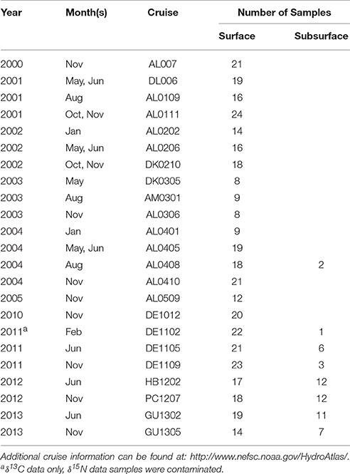
Table 1. Basic cruise information (year, month, cruise identifier) and number of samples collected from surface and subsurface waters.

FIGURE 1

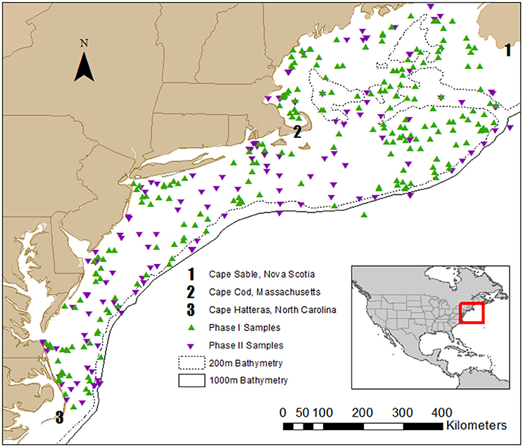
Figure 1. Map of Phase I (2000–2005) and Phase II (2010–2013) sample locations. The 200 and 1000 m bathymetry are included to illustrate the general location of the continental shelf, which is defined as the area from the coastline out to a water depth of 200 m.

TABLE 2

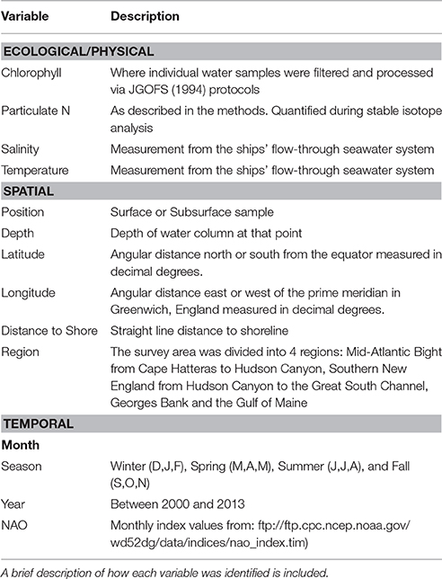
Table 2. Predictor variables used in random forest modeling.

For surface sample collection, an on-board flow-through seawater line was used to collect at least 200 ml of water which was first passed through a 300 μm mesh screen to remove zooplankton, and then through a pre-combusted glass fiber (GF/F, GE Whatman, gelifesciences.com) filter. For deep samples, a 10 L Niskin bottle (General Oceanics Inc., Miami, FL USA) was used to sample the bottom of the water column (to a maximum of 500 m) and the water captured by the Niskin was treated in the same manner as the surface seawater. Filters were frozen while the research cruise was underway. They were then dried in the lab in a 65°C oven for a minimum of 24 h. Once fully dry, filters were pelletized and analyzed on an Isotope Ratio Mass Spectrometer for δ¹⁵N and δ¹³C.

For surface chlorophyll-a (hereafter referred to as chlorophyll) samples, 200 ml of water was collected from the flow-through seawater line, passed through a 300 μm mesh screen and then passed through a GF/F glass fiber filter. The glass fiber filter was then placed in 7 ml of 90% acetone and stored in the freezer for 24 h (JGOFS Protocols, 1994). The extracted chlorophyll was read using a Turner Designs 10-AU fluorometer (Turner Designs, San Jose, CA USA). A solid standard was used to correct for instrument drift each time a reading was taken. For deep samples down to a maximum of 500 m, a 200 ml sample was drawn from the Niskin bottle used for the isotope sample and the water captured was treated in the same manner as the surface seawater. To determine the chlorophyll a level, the reading of the blank 90% acetone was subtracted from the extracted sample reading and multiplied by the solid standard calibration value and the ratio of volume of water filtered to the volume of acetone used to extract the chlorophyll.

Particulate Analysis

The δ¹⁵N and particulate nitrogen (PN) content was determined using an Isoprime 100 Isotope Ratio Mass Spectrometer interfaced with a Micro Vario Elemental Analyzer (Elementar Americas, Mt. Laurel, NJ). The nitrogen (δ¹⁵N) isotope composition was expressed as a part per thousand (permil) deviation (‰) from air, while the carbon (δ¹³C) was referenced to Vienna PeeDee Belemnite where δX = [(R_sample − R_standard)/R_standard] × 10³, X is δ¹⁵N or δ¹³C, and R is the ratio of heavy to light isotope (¹⁵N: ¹⁴N, ¹³C: ¹²C). Samples were analyzed randomly in batches of ~30. We used laboratory working standards of cystine, urea, graphite, dogfish, and blue mussel tissues to check for instrument drift in each run and to correct for instrument offset. Instrument precision is better than 0.3‰. The PN content on the filter was calculated by comparing the peak area of the unknown sample to a standard curve of peak area vs. standard N content. To determine the PN concentration, the N content of the material retained on the filter was divided by the volume filtered.

Statistical Analysis

The full dataset that was used for all subsequent statistical analyses is open-access and can be found at: http://tinyurl.com/gu9r34e.

Random forest modeling of the full Phase II dataset (including surface and bottom data) was used to explore the spatial structure as well as the potential environmental drivers of isotope values (Table 2). Random forest is a machine learning technique that aggregates a multitude of decisions trees in order to obtain a consensus prediction of the response variable (Breiman, 2001). Each tree model is constructed based on a recursively bootstrapped sample of the full data and fit using a subsample of the predictor variables. The out-of-bag (OOB) data, or cases left out of the model, are then used as an unbiased estimate of error and also to estimate variable importance. This process is repeated numerous times; specifically, we created 1000 trees for each of our final models. Thus, this ensemble approach avoids overfitting the final model to the data. All random forest modeling was conducted in R v. 3.2.4 (R Core Team, 2016) specifically using the randomForest package (Liaw and Wiener, 2002). Predictor variables were developed to assess the potential drivers of temporal and spatial stable isotope variation (Table 2).

As stated above, the OOB data were used to robustly estimate the variable importance. For each regression tree, the OOB data were used as test data to quantify mean square error. Also, for the subsampled variables of the respective tree, each variable was iteratively randomly permuted and the change in prediction was recorded. Relatively small changes in mean square error would indicate that the variable had relatively little impact on the overall model function. Conversely, large changes indicate that a particular variable had large impacts on the model's predictive ability.

Finally, to look for relationships between δ¹⁵N and depth in the subsurface samples of the Phase II data, nonlinear regression was used.

Data Visualization

To create a visualization of continuous isotopes concentrations across the study area, we used kernel interpolation with barriers with the Phase I and Phase II surface data only. This approach is similar to a local polynomial interpolation that allows non-Euclidean measurement of distances between nearest neighbors. Specifically we used the generalized coastline layer as a barrier which forced an as-the-fish-swims distance measure. This analysis was conducted in ArcGIS v. 10.2 (ESRI, 2013). Because results of random forest analyses indicated that temporal variables (year, season) were not the primary drivers of the observed spatial patterns in δ¹⁵N and δ¹³C, we used all available surface data in the interpolations.

Results

The more recently collected Phase II particulate δ¹⁵N values ranged from 0.8 to 17.4‰, where surface δ¹⁵N values averaged 5.3 ± 1.5‰ (n = 130) and deeper δ¹⁵N values averaged 8.1 ± 3.2‰ (n = 51). The highest δ¹⁵N values were measured in the deeper water, although most subsurface values were <10‰ (Figure 2). The surface values were consistent with the Phase I data, in which surface values averaged 6.8 ± 1.1 and 4.7 ± 1.0‰ for nearshore and offshore sample locations, respectively (McKinney et al., 2010). The combined Phase I and Phase II surface values were used to create an interpolated surface that reflected higher δ¹⁵N values near the coast, south of Cape Cod (Figure 1). The kriged δ¹⁵N surface was constructed from 343 data points, where the mean error was 0.016 and the root-mean-square standardized error was 0.995 (Figure 3).

FIGURE 2

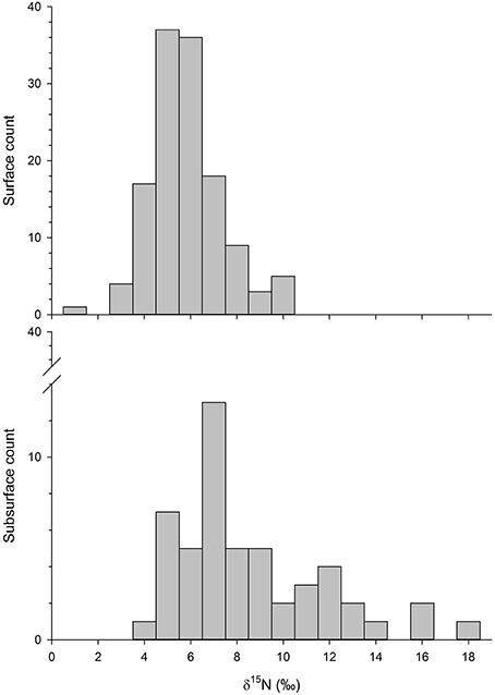
Figure 2. Histogram of surface and subsurface δ¹⁵N values from the Phase II dataset where the (top panel) shows the count of surface values and the (bottom panel) displays the count of measured subsurface δ¹⁵N values. Subsurface samples were collected at the bottom of the water column, or as far as the sampling cable would allow. Depths ranged from 17 to 508 m below the surface.

FIGURE 3

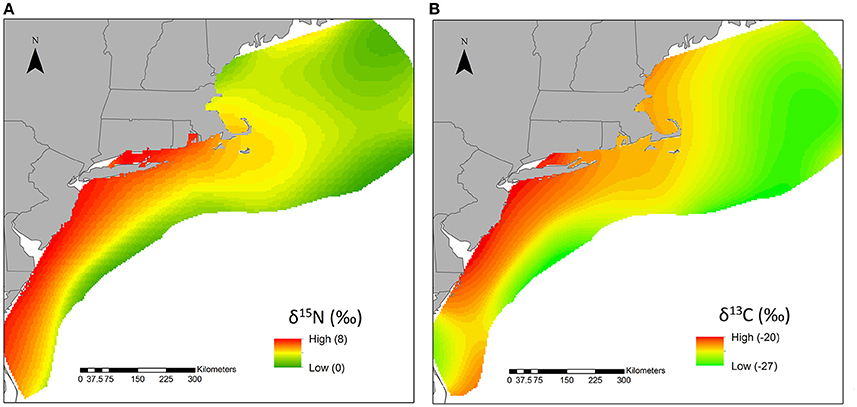
Figure 3. Interpolated surface of particulate nitrogen (A) and carbon (B) stable isotope values across the full study area. The gradient was scaled between the highest and lowest sampled values. The upper and lower bounds of δ¹⁵N and δ¹³C values were included in the legend to orient the reader. These values and the associated color gradations should not be used to quantify characteristic values for a particular region. Only samples collected from surface waters were included.

The δ¹³C values ranged from −26.4 to −15.6‰, where surface values averaged −22.8 ± 2.2‰ (n = 152) and bottom were −22.5 ± 2.6‰ (n = 52). The interpolated carbon surface was constructed from 160 points and had mean error of 0.078 and root-mean-square standardized error of 0.998. Overall, this kriged (spatially interpolated) surface was consistent with the δ¹⁵N surface, where higher values were observed closer to shore and lower values to the east and north of Cape Cod (Figure 3).

Random Forest

The final random forest models were built using exclusively Phase II data. The second phase of the data collection added carbon isotopes and chlorophyll concentrations, which allowed for an additional model beyond the nitrogen isotopes. These models included 158 Phase II data points that had all measurements for response and predictor variables. The carbon model explained 65% percent of the variance and has a mean-squared error of 1.96, while the nitrogen model explained 57% of the variance and had a mean-squared error of 2.70.

Chlorophyll concentration was the most important predictor of δ¹⁵N values, with higher chlorophyll associated with higher δ¹⁵N values (Figure 4A). The other stronger predictors of δ¹⁵N values were water column depth, position, particulate N, and distance to shore (Figure 4A). In general, subsurface water samples had higher δ¹⁵N than surface values; the highest values measured (>10‰) were from the deeper water samples (Figure 2). While subsurface δ¹⁵N values were significantly higher with depth (F = 16.6, P < 0.001), the relationship was coarse (R² = 0.27), where δ¹⁵N values at the shallowest depths (~20 m) ranged from 4 to 12‰ and from about 4–18‰ among the deepest samples (~500 m).

FIGURE 4

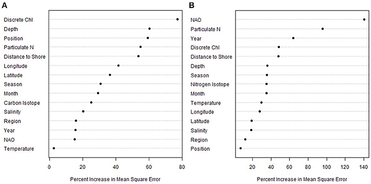
Figure 4. Variable importance plot of the Phase II particulate nitrogen (A) and carbon (B) random forest models. Plotted according to sorted percent increase mean square error; higher values indicate a higher influence on predicting particulate isotope values. See Table 2 for a description of categories.

The NAO index was the most important predictor of δ¹³C values, far beyond the other variables (Figure 4B), but this relationship appears to be primarily driven by high δ¹³C values from a research cruise (DE1102) conducted in a month with a very low NAO index (−2.25, Figure 5). These higher δ¹³C values were also positively correlated with the PN content of the filters, where PN was the second strongest predictor of δ¹³C values on the shelf. While year was also a strong predictor of δ¹³C values, this was likely also driven by the 2010 data, which had, on average, higher δ¹³C values than the other research cruises (as well as a very negative NAO index).

FIGURE 5

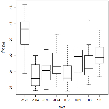
Figure 5. Boxplots of δ¹³C binned by North Atlantic Oscillation (NAO) index values (from ftp://ftp.cpc.ncep.noaa.gov/wd52dg/data/indices/nao_index.tim) where associated cruise numbers were (from left to right): HB1202, DE1012, DE1105, PC1207, DE1102, GU1305, GU1302, and DE1109. See Table 1 for details of corresponding sampling months and years.

Discussion

Overall, variability in the combined dataset was high, and results of the random forest analyses indicated that the variables with the greatest predictive capacities were different between δ¹⁵N and δ¹³C. This apparent disparity led us to develop a secondary goal of assessing the robustness of these patterns and bounding what can, and cannot, be said about the dataset. Overall, we propose that δ¹⁵N values were driven by a mix of continental runoff, upwelled, recycled, and fixed N, while differences in δ¹³C values reflected varying rates of production, with higher carbon isotope values associated with greater productivity.

Nitrogen Isotope Dynamics

Both high chlorophyll concentrations and high particulate N were indicators of higher productivity and, as suggested by this study, greater δ¹⁵N values. Our kriged image of all available surface nitrogen isotope data associated the highest surface values with near-shore areas and lower latitudes. Similar differences between higher nearshore and lower shelf edge δ¹⁵N values were seen in fish and invertebrates off the Newfoundland and Labrador coasts, northeast of our study area (Sherwood and Rose, 2005). Given that this portion of the Canadian coast was minimally developed, the authors didn't attribute the higher nearshore δ¹⁵N values to anthropogenic sources. Rather, they suggested that the observed differences may have been attributable to different productivity regimes, potentially associated with a range of processes, like the upwelling of nutrients (Sherwood and Rose, 2005). Similar patterns were also observed in our study area when we considered only the Phase I data (2001–2005; McKinney et al., 2010). McKinney et al. (2010) hypothesized that higher nearshore δ¹⁵N values are partially driven by continental and estuarine runoff. Estuaries and large rivers have been estimated to contribute between 464 and 627 × 10⁹ moles y⁻¹ to the continental shelves (<200 m deep) of the North Atlantic Ocean (Nixon et al., 1996), which was thought to be more than 20 times the potential contribution via biological N fixation (~20 × 10⁹ moles N y⁻¹). However, N upwelled from the continental slope was estimated to be much greater than all other sources combined, contributing between 2000 and 6000 × 10⁹ moles y⁻¹ (Nixon et al., 1996). Both terrestrial runoff and upwelled slope N may be contributing to the higher nearshore δ¹⁵N values.

In their review of larval transport mechanisms on the Northwest Atlantic continental shelf, Epifanio and Garvine (2001) identified the importance of buoyancy-driven flow and wind-driven upwelling circulation on larval transport. They describe north-to-south nearshore surface currents along the coast of the northeastern United States that transport fresher estuarine water south. This, combined with northward wind-driven upwelling, which brings nutrient-rich water into the photic zone, serve not just to transport larvae, but to support nearshore productivity (Epifanio and Garvine, 2001; Townsend et al., 2006). Deeper water tends to be more nutrient rich and to have higher δ¹⁵N values (e.g., Altabet, 1988). Our measurements of deeper water PM were consistent with this, as δ¹⁵N values tended to be higher at depth. The challenge in interpreting relative contributions of N from continental runoff and upwelling via δ¹⁵N values is that both are characterized by high δ¹⁵N values. Thus, while we can suggest that the higher δ¹⁵N values observed closer to shore may be attributable to some combination of these sources, we cannot parse out relative contributions. Contributions from both of these relatively higher nutrient sources would result in high isotope values close to shore, as well as high chlorophyll and PN concentrations. Our observed lower δ¹⁵N values north of Cape Cod and particularly in the Georges Bank are consistent with previously reported ranges, and may reflect differences in nitrogen dynamics related to temperature, or possibly differences in rates of upwelling (Fry, 1988; Wainright and Fry, 1994).

Carbon Isotope Dynamics

Relationships between carbon isotopes and productivity are fairly well established in both estuaries (Oczkowski et al., 2010, 2014) and the open ocean (Ostrom et al., 1997; Graham et al., 2010), where higher rates of primary production are associated with higher δ¹³C values. The random forest results were consistent with this, in which the NAO index and particulate N were the two biggest predictors of δ¹³C values. While higher amounts of particulate N indicate higher stocks of plankton in the water column, the link to NAO is more tenuous. The June 2012 data had, on average, higher δ¹³C values than the other cruises and coincided with a particularly strong NAO index (Figure 5). A very negative NAO phase is typically associated with colder and wetter, often snowier, weather in this region, which in turn can result in a greater than average spring freshet, but also with drier conditions in non-winter months. However, overall, hydrologic associations with the NAO are complex and difficult to generalize (Bradbury et al., 2002a,b; Pociask-Karteczka, 2006). In general, if δ¹³C values track production (e.g., Oczkowski et al., 2010, 2014), and production is impacted by the NAO, then a link between δ¹³C values and NAO phase is logical. However, we do not have the data to establish such a link and any such relationships are speculative.

In their review of open ocean isoscapes, Graham et al. (2010) observed that higher-latitude seas were often characterized by more negative δ¹³C values than lower latitudes. They correlated these spatial trends to lower photosynthetic rates associated with the colder regions. Our analyses also indicated a similar relationship between δ¹³C and geographic region. While admittedly coarse, results of kriging all available surface carbon isotope data show higher values closer to shore and in the mid-Atlantic region. These higher nearshore δ¹³C values may be reflecting relatively higher productivity supported by continental nutrient runoff and shoaling or upwelling of deeper, more nutrient rich waters, as described in association with higher δ¹⁵N values.

Broad Trends

There are clear similarities in spatial trends in the kriged surfaces for δ¹⁵N and δ¹³C values in particulate matter, where the highest values were observed closer to shore and south of Cape Cod. This is an area of (relatively) enhanced primary productivity that is supported by nutrients from continental runoff and upwelled from bottom waters. However, it is important to emphasize that it is not appropriate to use these surfaces to establish isoscapes or to identify specific values as characteristic of a region. The random forest modeling results indicated that neither distance from shore, nor water column depth, were particularly strong predictors of stable isotope values. This dataset challenges the assumption that offshore δ¹⁵N and δ¹³C values are uniform and suggests that we need to use caution when assuming characteristic isotopically low (δ¹⁵N < 6‰, δ¹³C < −20‰) shelf contributions to an estuary.

This relatively long time series of about twice yearly sampling of stable isotope (δ¹⁵N, δ¹³C) values from the Gulf of Maine to Cape Hatteras was undertaken to capture robust spatial patterns. Our sampling does not capture episodic events like spring blooms and warm core rings, which can have dramatic, if ephemeral, effects on δ¹⁵N and δ¹³C values. For example, while others have measured seasonal shifts in δ¹³C values associated with diatom blooms on Georges Bank, which is in the Gulf of Maine, our sampling did not capture them (Fry and Wainright, 1991; Wainright and Fry, 1994). As another example, detailed documentation of δ¹⁵N values in particulate nitrogen in warm core rings, which were generally observed at the edge or to the east of our study area, demonstrate a shift of up to 8‰ associated with stratification in these rings (Altabet and McCarthy, 1985). Even more dramatically, δ¹⁵N values of up to 40‰ were observed in the particulate N collected from the center of these rings. Despite this, our results can provide some insight into large scale stable nitrogen and carbon isotope dynamics in continental shelf waters, and hence help fill the data gap between estuarine and open ocean studies. While tentative, the possible link between δ¹³C values and large-scale climate oscillations (e.g., the NAO) is intriguing and suggests that spatially and temporally explicit stable isotope measurements made in surface phytoplankton could record global perturbations.

Author Contributions

AO and RM developed the hypothesis, JP obtained the samples, while AO, JP, and RM analyzed the samples. BK did all of the data analysis and all authors contributed to manuscript development.

Funding

This research was funded in part by the US Environmental Protection Agency and the US National Oceanic and Atmospheric Administration.

Conflict of Interest Statement

The authors declare that the research was conducted in the absence of any commercial or financial relationships that could be construed as a potential conflict of interest.

Acknowledgments

We thank Erin Markham for help processing samples, and the staff and volunteers on the research cruises for helping to collect and process the samples, and John Kiddon for input on Cape Cod identification. The manuscript was improved by comments from Rich Pruell, Alana Hanson, and Anne Kuhn. This is ORD Tracking Number ORD-018002 of the Atlantic Ecology Division, National Health and Environmental Effects Research Laboratory, Office of Research and Development, U.S. Environmental Protection Agency. The research described in this article has been funded in part by the U.S. Environmental Protection Agency. This document has been reviewed by the U.S. Environmental Protection Agency, Office of Research and Development, and approved for publication. Mention of trade names or commercial products does not constitute endorsement or recommendation for use.

References

Abend, A. G., and Smith, T. D. (1997). Differences in stable isotope ratios of carbon and nitrogen between long-finned pilot whales (Globicephala melas) and their primary prey in the western north Atlantic. ICES J. Mar. Sci. 54, 500–503. doi: 10.1006/jmsc.1996.0192

CrossRef Full Text | Google Scholar

Altabet, M. (1988). Variations in nitrogen isotopic composition between sinking and suspended particles: implications for nitrogen cycling and particle transformation in the open ocean. Deep Sea Res. Part A Oceanogr. Res. Pap. 35, 535–554. doi: 10.1016/0198-0149(88)90130-6

CrossRef Full Text | Google Scholar

Altabet, M. A., and McCarthy, J. J. (1985). Temporal and spatial variations in the natural abundance of ¹⁵N in PON from a warm-core ring. Deep Sea Res. Part A Oceanogr. Res. Pap. 32, 755–772. doi: 10.1016/0198-0149(85)90113-X

CrossRef Full Text | Google Scholar

Bradbury, J. A., Dingman, S. L., and Keim, B. D. (2002a). New England drought and relations with large scale atmospheric circulation patterns. J. Am. Water Resour. Assoc. 38, 1287–1299. doi: 10.1111/j.1752-1688.2002.tb04348.x

CrossRef Full Text | Google Scholar

Bradbury, J. A., Keim, B. D., and Wake, C. P. (2002b). US East Coast trough indices at 500 hPa and New England winter climate variability. J. Clim. 15, 3509–3517. doi: 10.1175/1520-0442(2002)015<3509:USECTI>2.0.CO;2

CrossRef Full Text | Google Scholar

Breiman, L. (2001). Random forests. Mach. Learn. 45, 5–32. doi: 10.1023/A:1010933404324

CrossRef Full Text | Google Scholar

Casciotti, K., Trull, T., Glover, D., and Davies, D. (2008). Constraints on nitrogen cycling at the subtropical North Pacific Station ALOHA from isotopic measurements of nitrate and particulate nitrogen. Deep Sea Res. Part II Top. Stud. Oceanogr. 55, 1661–1672. doi: 10.1016/j.dsr2.2008.04.017

CrossRef Full Text | Google Scholar

Ceriani, S. A., Roth, J. D., Evans, D. R., Weishampel, J. F., and Ehrhart, L. M. (2012). Inferring foraging areas of nesting loggerhead turtles using satellite telemetry and stable isotopes. PLoS ONE 7:e45335. doi: 10.1371/journal.pone.0045335

PubMed Abstract | CrossRef Full Text | Google Scholar

Costanzo, S. D., O'Donohue, M. J., and Dennison, W. C. (2003). Assessing the seasonal influence of sewage and agricultural nutrient inputs in a subtropical river estuary. Estuaries 26, 857–865. doi: 10.1007/BF02803344

CrossRef Full Text | Google Scholar

Epifanio, C., and Garvine, R. (2001). Larval transport on the Atlantic continental shelf of North America: a review. Estuar. Coast. Shelf Sci. 52, 51–77. doi: 10.1006/ecss.2000.0727

CrossRef Full Text | Google Scholar

ESRI (2013). ArcGIS Desktop: Release 10.2. Redlands, CA: Environmental Systems Research Institute.

Fry, B. (1983). Fish and shrimp migrations in the Northern Gulf of Mexico analyzed using stable C, N, and S isotope ratios. Fish. Bull. 81, 789–801.

Google Scholar

Fry, B. (1988). Food web structure on Georges Bank from stable C, N, and S isotopic compositions. Limnol. Oceanogr. 33, 1182–1190.

Google Scholar

Fry, B., and Wainright, S. C. (1991). Diatom sources of 13C-rich carbon in marine food webs. Mar. Ecol. Prog. Ser. 76, 149–157. doi: 10.3354/meps076149

CrossRef Full Text | Google Scholar

Gearing, P., Plucker, F. E., and Parker, P. (1977). Organic carbon stable isotope ratios of continental margin sediments. Mar. Chem. 5, 251–266. doi: 10.1016/0304-4203(77)90020-2

CrossRef Full Text | Google Scholar

Graham, B. S., Koch, P. L., Newsome, S. D., McMahon, K. W., and Aurioles, D. (2010). “Using isoscapes to trace the movements and foraging behavior of top predators in oceanic ecosystems,” in Isoscapes, eds J. B. West, J. L. Bowen, T. E. Dawson, and K. P. Tu (Dordrecht: Springer), 299–318.

JGOFS Protocols (1994). Chapter 14. Measurement of Chlorophyll a and Phaeopigments by Fluorometric Analysis. Available online at: http://ijgofs.whoi.edu/Publications/Report_Series/JGOFS_19.pdf

Liaw, A., and Wiener, M. (2002). Classification and Regression by randomForest. R News 2, 18–22.

Google Scholar

McKinney, R., Oczkowski, A., Prezioso, J., and Hyde, K. (2010). Spatial variability of nitrogen isotope ratios of particulate material from Northwest Atlantic continental shelf waters. Estuar. Coast. Shelf Sci. 89, 287–293. doi: 10.1016/j.ecss.2010.08.004

CrossRef Full Text | Google Scholar

McMahon, K. W., Ling Hamaday, L., and Thorrold, S. R. (2013). A review of ecogeochemistry approaches to estimating movements of marine animals. Limnol. Oceanogr. 58, 697–714. doi: 10.4319/lo.2013.58.2.0697

CrossRef Full Text | Google Scholar

Nixon, S., Ammerman, J., Atkinson, L., Berounsky, V., Billen, G., Boicourt, W., et al. (1996). The fate of nitrogen and phosphorus at the land-sea margin of the North Atlantic Ocean. Biogeochemistry 35, 141–180. doi: 10.1007/BF02179826

CrossRef Full Text | Google Scholar

Oczkowski, A., Markham, E., Hanson, A., and Wigand, C. (2014). Carbon stable isotopes as indicators of coastal eutrophication. Ecol. Appl. 24, 457–466. doi: 10.1890/13-0365.1

PubMed Abstract | CrossRef Full Text | Google Scholar

Oczkowski, A., Nixon, S., Henry, K., DiMilla, P., Pilson, M., Granger, S., et al. (2008). Distribution and trophic importance of anthropogenic nitrogen in Narragansett Bay: an assessment using stable isotopes. Estuar. Coasts 31, 53–69. doi: 10.1007/s12237-007-9029-0

CrossRef Full Text | Google Scholar

Oczkowski, A. J., Pilson, M. E., and Nixon, S. W. (2010). A marked gradient in δ13C values of clams Mercenaria mercenaria across a marine embayment may reflect variations in ecosystem metabolism. Mar. Ecol. Prog. Ser. 414, 145–153. doi: 10.3354/meps08737

CrossRef Full Text | Google Scholar

Ostrom, N. E., MacKo, S. A., Deibel, D., and Thompson, R. J. (1997). Seasonal variation in the stable carbon and nitrogen isotope biogeochemistry of a coastal cold ocean environment. Geochim. Cosmochim. Acta 61, 2929–2942. doi: 10.1016/S0016-7037(97)00131-2

CrossRef Full Text | Google Scholar

Pantoja, S., Repeta, D. J., Sachs, J. P., and Sigman, D. M. (2002). Stable isotope constraints on the nitrogen cycle of the Mediterranean Sea water column. Deep Sea Res. Part I Oceanogr. Res. Pap. 49, 1609–1621. doi: 10.1016/S0967-0637(02)00066-3

CrossRef Full Text | Google Scholar

Peters, K., Sweeney, R., and Kaplan, I. (1978). Correlation of carbon and nitrogen stable isotope ratios in sedimentary organic matter. Limnol. Oceanogr. 23, 598–604. doi: 10.4319/lo.1978.23.4.0598

CrossRef Full Text | Google Scholar

Pociask-Karteczka, J. (2006). River hydrology and the North Atlantic oscillation: a general review. AMBIO J. Hum. Environ. 35, 312–314. doi: 10.1579/05-S-114.1

CrossRef Full Text | Google Scholar

R Core Team (2016). ArcGIS Desktop: Release 10.2. Redlands, CA: Environmental Systems Research Institute.

Sherwood, G. D., and Rose, G. A. (2005). Stable isotope analysis of some representative fish and invertebrates of the Newfoundland and Labrador continental shelf food web. Estuar. Coast. Shelf Sci. 63, 537–549. doi: 10.1016/j.ecss.2004.12.010

CrossRef Full Text | Google Scholar

Sigman, D., Altabet, M., McCorkle, D., Francois, R., and Fischer, G. (2000). The δ¹⁵N of nitrate in the Southern Ocean: nitrogen cycling and circulation in the ocean interior. J. Geophys. Res. 105, 19599–19614. doi: 10.1029/2000JC000265

CrossRef Full Text | Google Scholar

Townsend, D. W., Thomas, A. C., Mayer, L. M., Thomas, M. A., and Quinlan, J. A. (2006). “Oceanography of the northwest Atlantic continental shelf (1, W),” in The Sea: The Global Coastal Ocean: Interdisciplinary Regional Studies and Syntheses, Vol. 14, eds A. R. Robinson and K. H. Brink (Cambridge: Harvard University Press), 119–168.

Wainright, S. C., and Fry, B. (1994). Seasonal variation of the stable isotopic compositions of coastal marine plankton from Woods Hole, Massachusetts and Georges Bank. Estuaries 17, 552–560. doi: 10.2307/1352403

CrossRef Full Text | Google Scholar