Kinneyia: A Flow-Induced Anisotropic Fossil Pattern from Ancient Microbial Mats

1. Introduction

1.1. Biofilms and Microbial Mats

Biofilms are dense microbial colonies covering solid surfaces. They are found in vastly variable environments, ranging from deep sea hydrothermal vents (Wolff, 1977) to the Antarctic (Friedmann and Weed, 1987; Hawes et al., 2013), sewage pipes, and even the human body (Hall-Stoodley and Stoodley, 2009). They represent, however, not only one of the most ubiquitous life forms on Earth but also one of the earliest. Recent discoveries provide evidence that fossils of microbial origin date back at least 3.45 billion years (Allwood et al., 2006), suggesting that biofilms have been present throughout the majority of Earth’s history.

Microbial mats (MM) may be viewed as thick biofilms. Their thickness ranges from a few millimeters to about a centimeter, depending on habitat, growth conditions, and on the microbial species they consist of (Neu and Lawrence, 1997; Gerdes et al., 2000). These may include bacteria, archaea (Zolghadr et al., 2010), protozoans, algae (de Brouwer et al., 2005), and fungi (Verstrepen and Klis, 2006). Due to the lack of large-scale internal organization, the material MM consist of appears rather homogeneous. While the distribution of microbial species exhibits a pronounced vertical stratification (with phototrophic species prevailing in the top region and sulfur breathing species in the anoxic deeper layers), they are generally rather featureless and isotropic with respect to the plane of the substrate they grow on.

As a consequence, the primary evidence of ancient MM is not a topographic feature, as in many other fossils, but the mineral content of the adjacent sedimentary layers, and peculiarities in the sedimentary grain size distribution. In ancient siliciclastic biolaminates, former microbial mats are indicated by black carbonaceous materials (Noffke et al., 2002; Bouougri and Porada, 2007; Noffke, 2010), pyrite (Pfluger and Gresse, 1996), and darker layers rich in iron-oxides. In modern MM, these compounds are produced by the metabolic activity of microorganisms living in and below the mat (Dupraz et al., 2004; Schieber and Glamoclija, 2007; Sarkar et al., 2008). There are, however, a class of microbially induced sedimentary structures (MISS) that show up as topographic features on the bedding planes, which formerly carried the MM (Schieber, 2007; Schieber et al., 2007). In these cases, the inherent isotropic symmetry of the MM has been broken, and in some cases the underlying mechanisms are still elusive. The present paper addresses some physical aspects of MISS exhibiting a pronounced anisotropy (called Kinneyia, see below) the formation of which has been unclear to date.

1.2. Physical Properties of Microbial Mats

MM are held together by extracellular polymeric substances (EPS) (Wingender et al., 1999), which are produced by microbes. These substances bestow mechanical stability to the colony and make up 50–90% of the total organic material in the film (Flemming and Wingender, 2010). They are responsible for adhesion of the mat to surfaces (Donlan, 2002; Flemming and Wingender, 2010) and provide a mechanically stable scaffold for the microbial colony (Mayer et al., 1999). One may, therefore, anticipate that EPS largely determine the physical properties of MM.

In fact, modern biofilms and microbial mats are found to behave like viscoelastic films (Shaw et al., 2004; Vinogradov et al., 2004; Rupp et al., 2005; Lieleg et al., 2011). Lieleg et al. (2011) have shown that biofilms display elastic-like responses for high frequency stimuli, and viscous-fluid responses when low frequency mechanical stimuli are applied. In the context of MM, this means that for short-term exposure to shear stress the mat responds elastically. For sustained exposure to shear stress, on the other hand, internal physical stresses are dissipated through viscous flow. Although the composition of EPS may vary widely, recent investigations of modern microbial mats have revealed a number of well-conserved features. While the viscosity η, and shear modulus G, of biofilms are seen to vary by over seven orders of magnitude (Shaw et al., 2004), the stress relaxation time, τ = η/G, is strikingly well conserved, being generally found to be between about 10 and 30 min. This relaxation time is thought to be the typical lifetime of the temporary crosslinks in the EPS. Comparative studies of modern and ancient microbial structures suggest that ancient microorganisms existed with the same diversity as today (Noffke, 2010). It is, therefore, not unreasonable to assume far reaching similarities in the general material characteristics of ancient and modern microbial mats. This shall serve as a working hypothesis throughout the present paper.

2. Kinneyia

Given the lateral homogeneity of MM, it is surprising that some fossil MISS connected to MM exhibit a very pronounced spatial pattern. The focus of the present paper is a particularly prominent representative called Kinneyia (Porada and Bouougri, 2007; Porada et al., 2008). It is found predominantly on the upper bedding planes of sandstone or siltstone layers, which can be identified as storm wave deposits in formerly littoral areas. It is characterized by an undulating ripple-like structure (Figure 1) with a wavelength typically between 2 and 20 mm. The ripple shape tends to deviate slightly from a sinusoidal wave, commonly with flattened crests and rounded troughs, but sometimes also with rounded and even sawtooth-shaped crests (Porada et al., 2008). The relative widths of the troughs and the ridges vary widely from sample to sample (Pfluger, 1999). The ripple pattern is generally well ordered, with the crests orientated parallel to one another. Honeycomb-like patterns with round or elongated pits are also seen (Figure 1C). Both morphologies often coexist on different areas of the same outcrop (Hagadorn and Bottjer, 1999; Porada and Bouougri, 2007). We note that there is a variety of similar structures the biological origin of which is at least controversial (Davies et al., 2016). In the present paper, we focus on those fossil structures that can be clearly identified as MISS.

FIGURE 1

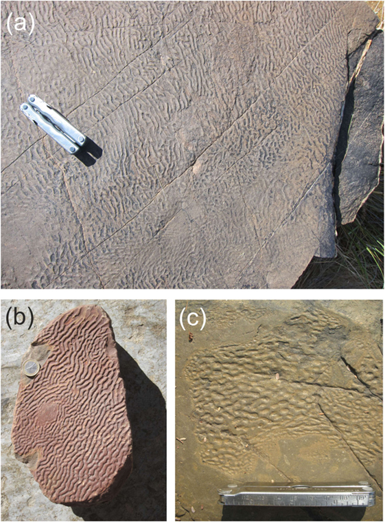
Figure 1. Proterozoic Kinneyia structures from Neuras and Haruchas farms, Namibia. While the Neuras facies (A,B) displays large (>1 m²) areas covered with clearly oriented ripples, the Haruchas facies (C) is rather characterized by small (≈10 cm across) patches of honeycomb-like structures.

The examples shown in Figure 1 are from two outcrops in Namibia. They date to the terminal Proterozoic Vingerbreek Member, Schwarzrand Subgroup, Nama Group. The first site was located at Neuras farm [24° 24′ 11.3″ S; 16° 15′ 8.7″ E]. The Kinneyia here are found on two isolated outcrops located on a cliff overlooking a river bed. The second fossil site was located at Haruchas farm [24° 21′ 46.3″ S; 16° 24′ 21.6″ E] (Noffke et al., 2002; Bouougri and Porada, 2007). The outcrop is ~3 × 6 m in area and is covered with small Kinneyia patches (e.g., Figure 1C).

In order to gain detailed data on the topography of the fossils, mold casts have been prepared in the field and analyzed by standard profilometry in the laboratory (Thomas et al., 2013). Figure 2 shows results for the crest-to-valley amplitude as a function of the ripple wavelength for a number of samples from both Neuras and Haruchas (open circles). The symbol size roughly corresponds to the experimental error. It is interesting to note that there is a roughly linear relation between the wavelength of the ripple and its crest-to-valley amplitude. The inset shows a few sample traces, demonstrating the flattened crests and troughs frequently found in Kinneyia fossils.

FIGURE 2

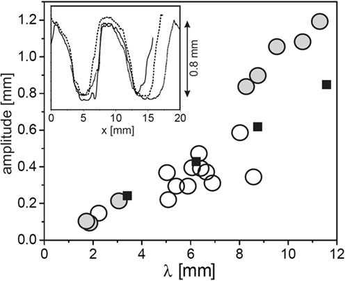
Figure 2. Topographic characteristics of Kinneyia fossils and their models generated in the laboratory. Circles: crest-to-valley amplitude of Kinneyia ripples as a function of their wavelength for fossils from Namibia (Neuras (gray) and Haruchas (white) outcrop). The symbol size roughly corresponds to the observational error. Squares: saturation amplitudes of artificial Kinneyia structures generated in the laboratory. Inset: sample profiles as taken from a fossil mold cast [adapted with modifications from Thomas et al. (2013)].

Kinneyia outcrops have been dated from as early as 2.9 Ga ago (Noffke et al., 2003a), and occur at virtually all times well into the Mesozoic. In the course of the Mesozoic, they gradually become more scarce in the fossil record, with the latest representatives being reported from the Jurassic. Because of the frequent occurrence of Kinneyia in fossils from over three billion years, as well as because of their gradual disappearance during the Mesozoic, Kinneyia could be very informative for paleontologic studies. Consequently, it is extremely desirable to understand how Kinneyia structures are created from MM.

3. Suggested Mechanisms for Kinneyia Formation

After early attempts to interpret Kinneyia by abiotic mechanisms (Shrock, 1948; Allen, 1966; Singh and Wunderlich, 1978) had been shown to be inconclusive, Hagadorn and Bottjer (1997, 1999) were the first to suggest that the formation of Kinneyia may involve microbial mats. Note that the ripples of Kinneyia are often seen to have very steep slopes, such as seen in the inset of Figure 2, which would be unstable without some “glue,” such as EPS, to bind the grains together.

Pflüger later proposed a microbially mediated gas bubble model for Kinneyia formation (Pfluger, 1999). He suggested that gas rising up from a sedimentary substrate can be trapped by a MM, and collect to form bubbles below the MM. Using a mixture of water-saturated sand and sodium bicarbonate, Pflüger indeed observed that bubbles (of CO₂) destabilized the sediment and thereby left trace patterns.

Indications of bubbles rising below MM are indeed known. Gas domes, polydisperse round shapes up to tens of centimeters in diameter, are observed in modern and ancient microbial mats (Gerdes, 2007). However, as their patterns do not correspond well with the well-defined elongated ridge and trough structures of Kinneyia, gas domes are no longer thought to be responsible for Kinneyia formation. Although Pflüger did not refer explicitly to gas domes mediating the destabilization of the MM, an alternative model of how gas bubbles below the mat would lead to a ripple-like destabilization was not provided. Furthermore, it is hard to conceive of a structure as regular as those shown in Figures 1A,B as being formed by gas bubbles.

3.1. The Liquefied Sediment (LS) Model

A different model for the development of Kinneyia has been put forward by Porada et al. (2008), who proposed that the pattern forms in liquefied sediment (LS) confined beneath microbial mats. Similar to Pflüger (Pfluger, 1999), Porada et al. assumed the microbial mat to act as a barrier to gas and groundwater trapped in the underlying sediment. In this model, however, the bacteria are assumed to form dispersed colonies in the sediments, in regions where the mats have adhered to the substrate and grown downwards. The gas then accumulates between the colonies within the pore space, leading to local anisotropies on the microscale in the elsewhere water-saturated sediment. Oscillating water flow from tidal currents may give rise to cyclic stressing, causing the underlying sediments to liquefy due to the oscillating pore pressure. The liquefied sand layer is assumed to be several centimeters thick with the overlying mat being up to 3-cm thick. The oscillatory pressure changes induce ripple structures in both the liquefied sand and microbial mat. The wavelength of the ripples is on the order of 1 m for the sand and a few centimeters for the mat. The ripple pattern in the mat induces further local variations in the pore pressure causing seepage and grain lifting. If the LS layer becomes very thin, then replication of the overlying small wavelength microbial ripples can occur in this underlying liquefied layer. This condition is satisfied periodically at the seaward boundary of the mat during each tidal cycle.

In the model of Porada et al. (2008), the small-scale ripple patterns are induced at the boundary between the overlying mat and the underlying sediment. Observation of modern microbial mats, however, suggests that it is not always possible to make a clear distinction between these two layers. Mats are often seen to develop from biofilms that initially form around individual sediment grains and subsequently grow together into a thick layer. Hence, the sediments are an integral part of the microbial mat. This is the case in particular for mats growing after storm floods, because then microbes and mineral particles are simultaneously deposited by sedimentation. It should be noted that such events are thought to be favorable for the scenario envisaged by Porada et al. (2008), as they provide the increased water head that is necessary to create aqueous flow below the MM, which may lead to fluidisation of the sediment.

3.2. The Oscillatory Flow (OF) Model

In a recent publication (Mariotti et al., 2014), Mariotti and coworkers proposed a new model that considers the effect of the oscillating flow (OF) at the bottom of a water body due to occasionally excited surface waves. They argued that in the presence of lumps of microbial aggregates, which frequently reside close to the sea floor due to their being slightly heavier than the surrounding water, light motion of the water may lead to ripple patterns in the sand at the bottom, very reminiscent of what we find as Kinneyia in the fossil record.

3.2.1. The Mechanism

The mechanism works as follows. Microbial material settling to the sea floor will predominantly accumulate in the troughs of the sediment bedding. Any Fourier component in the topography of the sea floor thus leads, through the effect of gravity, to a corresponding modulation of the density of the microbial aggregates. When the latter are moved back and forth in an oscillatory manner with an amplitude a, only Fourier components belonging to a wavelength λ = 2a (or multiples thereof) will lead to an average density variation under this motion. As a consequence, the slight buoyancy difference between the water and the microbial aggregates will, over time, lead to an enhancement of periodic depressions that have the corresponding spacing. Hence, any initial variation in the seafloor topography, with a wavelength near 2a, has a propensity to be amplified. Its amplitude will thus grow with time, and a well-defined ripple with a wavelength of λ ≈ 2a is expected to emerge.

This is observed in their experiments. To model a shallow tidal pool, lagoon, or lake, the authors used a ≈ 75-cm-long water tank. The conditions of water flow at the bottom were adjusted by varying the amplitude of a sloshing motion induced externally on the water in the tank. They let aggregates of microbial matter sink to the bottom of the container. After 24 h of sloshing with a constant amplitude, ripples reminiscent of Kinneyia indeed formed (cf. inset of Figure 3).

FIGURE 3

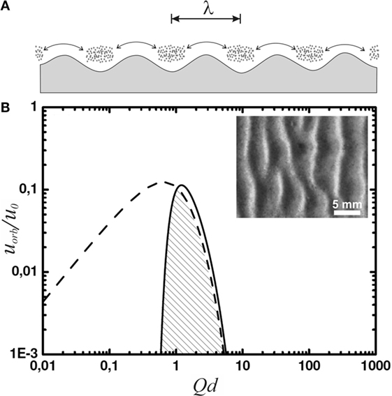
Figure 3. (A) Sketch of lumps of microbial material at the sea floor, agitated in an oscillatory manner with a peak-to-peak amplitude indicated by the double arrow. Gravity accumulates microbial material in the troughs of the sea floor profile, and the lumps thus forming deepen in turn the sea floor troughs. (B) The orbital velocity spectrum (solid curve) and its limit due to wave breaking (dashed curve). The inset shows a top view of a ripple obtained in the corresponding experiments [adapted with modification from ref. Mariotti et al. (2014)].

3.2.2. Predictions of the Model

In order to assess the predictive power of this model, we have to take a closer look at the experimental conditions under which it has been tested. The geometry of the container determined the frequency of sloshing, and hence of the liquid motion the microbial aggregates experienced at the bottom of the container. In a field situation, however, there is no such geometric limitation, and the liquid motion, excited by wind and tidal currents, will extend over a spectrum of frequencies. It is well established that waves on deep water can be represented by the so-called Pierson–Moskowitz spectrum (Liu, 1985; Bergdahl, 2009),

$S_{\text{PM}}\left(\mathrm{\omega }\right)\propto {\mathrm{\omega }}^{-5}{\exp }^{-\mathrm{\beta }{\mathrm{\omega }}^{-4}},$ (1)

where S is the spectral density of the mean square amplitude, ω is the (angular) frequency of the waves, and β is a fitting parameter. For shallow water, it has been shown that this spectrum has to be multiplied by a function ϕ(ω/ω₀), where ${\mathrm{\omega }}_0=\sqrt{2g∕d}$ (g is the acceleration due to gravity, d is the depth of the water) (Bergdahl, 2009). At low frequencies, $\mathrm{\varphi }\approx {\mathrm{\omega }}^2∕{\mathrm{\omega }}_0^2$, while for ω ≫ ω₀ it approaches unity. Here, we use $\mathrm{\varphi }={\tanh }^2\frac{\mathrm{\omega }}{{\mathrm{\omega }}_0}$. The result is the so-called TMA spectrum for finite depth water (Bergdahl, 2009),

$S_{\text{TMA}}\left(\mathrm{\omega }\right)\propto {\tanh }^2\left(\frac{\mathrm{\omega }}{{\mathrm{\omega }}_0}\right){\left(\frac{{\mathrm{\omega }}_0}{\mathrm{\omega }}\right)}^5{\exp }^{-\frac{5}{16}{\left(\frac{{\mathrm{\omega }}_0}{\mathrm{\omega }}\right)}^4}.$ (2)

This can be related to the wave number, Q = 2π/λ, through the dispersion relation of shallow water waves (Landau and Lifshitz, 1959),

$\mathrm{\omega }={\mathrm{\omega }}_0\sqrt{\frac{\mathit{Qd}}{2}\tanh \left(\mathit{Qd}\right)}.$ (3)

Since we are interested in the fluid motion at the bottom of the lagoon or lake, we still have to multiply by e^−Qd, which accounts for the decay of the fluid motion with depth. The result in terms of the orbital velocity, u_orb, is shown as the solid curve in Figure 3 with reference to $u_0=\sqrt{\mathit{gd}}$, which provides a natural velocity scale of the system. The spectrum is characterized by a quite narrow peak around Qd ≈ 1. Spectral functions representing experimental data more closely than Pierson–Moskowitz or TMA are known to be even more strongly peaked (Liu, 1985; Bergdahl, 2009). As a result, we see that the spectrum of waves is strongly dominated by waves with

$\mathrm{\omega }\approx \sqrt{\frac{g\tanh 1}{d}}\approx 0.62{\mathrm{\omega }}_0.$ (4)

Next we consider the absolute values of the amplitudes we expect. An upper limit is provided by wave breaking, which is known (Miche, 1951; Mariotti et al., 2014) to happen at

$h_{\text{wb}}=0.88d\frac{\tanh \mathit{Qd}}{\mathit{Qd}}.$ (5)

The corresponding orbital velocity at the bottom is

$u_{\text{wb}}=\frac{h_{\text{wb}}}{2}\mathrm{\omega }{e}^{-\mathit{Qd}}=0.44u_0\frac{{\left(\tanh \mathit{Qd}\right)}^{3∕2}}{\sqrt{\mathit{Qd}}{e}^{\mathit{Qd}}}.$ (6)

This is plotted as the dashed curve in Figure 3. The amplitude of the spectrum (solid curve) has been adjusted such that its dominant modes have just reached the wave breaking limit. Since the right wing of the spectrum almost coincides with the dashed curve, we see that wave breaking will not noticeably change the overall spectrum, nor the wave number of its dominant modes around Qd ≈ 1. The velocity amplitude, i.e., the orbital velocity, of the latter is limited to about u ≤ 0.1 u₀.

Numerical values of u₀ are plotted in the inset in Figure 4 as a function of depth (solid line). These are to be compared with the orbital velocities that are relevant to the formation of ripples in the framework of the OF model (Mariotti et al., 2014). Experimentally, it was found that below orbital velocities of about 2 cm/s, no ripples formed; while at orbital velocities above 8 cm/s, abiotic structures emerged, rendering the microbial matter irrelevant. This range is indicated by the gray bar. The dotted line at 0.1 u₀ represents the wave breaking limit. The velocities relevant to the model are in general much smaller than those prevailing close to the wave breaking limit anywhere in the important range of water depth. For ripple formation according to the OF model, we thus have to envisage rather soft agitation of the water, well below the wave breaking limit. This limit can be safely disregarded for the present system.

FIGURE 4

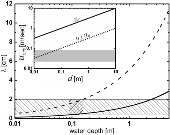
Figure 4. The prediction of the oscillating flow model for the wavelength of the Kinneyia pattern. The hatched region indicates the observed wavelengths, while the cross-hatched region indicates the region of water depth for which the predictions of the OF model agree with the observations from the fossil record. The inset shows the orbital velocity at the bottom, u_orb, as a function of water depth, d. According to Figure 3, the dashed line representing u_orb = 0.1 u₀ is relevant. The gray shaded area represents orbital velocities relevant to the OF model. For any depth of the water body larger than about 8 cm, wave breaking is clearly irrelevant to the OF mechanism.

Now, we turn to the wavelength of the emerging ripple pattern, λ. According to the model, it is directly related to the amplitude at the bottom, such that we can write the orbital velocity as

$u=\frac{1}{2}\mathrm{\lambda \omega }.$ (7)

From the discussion above (cf. Figure 3), we know that the motion at the bottom is dominated by modes with Qd ≈ 1. This allows to calculate the dominant sloshing frequency, and hence λ, once u is given. The result is

$\mathrm{\lambda }=2u\sqrt{\frac{d}{g\tanh 1}}.$ (8)

If we do this for both the minimum orbital velocity, u_min = 2 cm/s, below which no ripples form, and for the maximum orbital velocity, u_max = 8 cm/s, above which abiotic processes dominate, we arrive at a prediction for the range of λ for the OF model. Figure 4 shows the lower (solid curve) and upper (dashed curve) boundaries for λ as a function of the water depth. Clearly, the wavelengths observed in Kinneyia fossils, which are indicated by the hatched region, are correctly predicted only for water depths around 10 cm (cross-hatched). At depths above about 40 cm, the predicted range overlaps only by 50% with the observation, similarly for depths below about 2 cm. When the water body is deeper than about 2 m, there is no accordance of the prediction of the OF model with field evidence.

3.3. The Hydrodynamic Instability (HI) Model

We have recently proposed a particularly simple model for the formation of Kinneyia ripple patterns, which is based on a flow-induced hydrodynamic instability (HI) (Thomas et al., 2013). The HI naturally gives rise to an undulating structure on the length scales typical of Kinneyia. Evidence from analog experiments has been presented and compared with detailed measurements of fossilized Kinneyia, and shall be briefly reviewed here.

Kinneyia are generally found on upper bedding planes in littoral environments. For the purposes of the HI model, we shall, therefore, consider a planar microbial mat on a solid substrate subject to some flow in the overlying fluid (Figure 5A). The microbial mat is considered to behave as a viscoelastic fluid (Shaw et al., 2004).

FIGURE 5

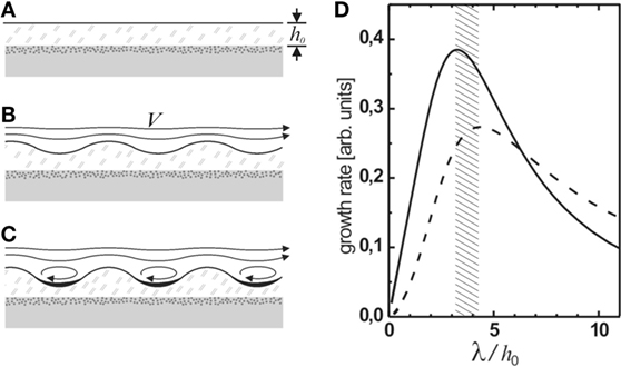
Figure 5. (A–C) Schematic representation of the generation of Kinneyia-type ripples from a hydrodynamic instability (HI). The microbial mat grows in a quiescent environment and is then subject to significant flow in the overlying water (A). This results in a HI, which gives rise to a ripple pattern at the surface of the mat (B). Once the amplitude of the ripple reaches a certain threshold, eddies will form in the valleys giving rise to stagnation points and enhanced sedimentation (C). Rupture of the film can occur when the amplitude of the troughs becomes comparable to the film thickness. (D) The predicted relative growth rate of the ripple pattern is sharply peaked around a dominant wavelength of 3.2 to 4.3 times the film thickness h₀ [adapted from Thomas et al. (2013) with modifications].

It is well known that spontaneous destabilization of a fluid–fluid interface may occur in a two-fluid system if the layers respond differently to shear (Landau and Lifshitz, 1959). A well-defined instability occurs, giving rise to a harmonic interfacial corrugation (Figure 5B). This HI occurs ubiquitously in nature (Hasegawa et al., 2004; Casanova et al., 2011; Smyth and Moum, 2012), for example, in cloud layers (Dalin et al., 2010), in which case it is referred to as the Kelvin–Helmholtz instability (Landau and Lifshitz, 1959).

3.3.1. The Mechanism

The system being studied is sketched in Figure 5. Water flows with far-field velocity V in the x-direction over a viscoelastic film of thickness h₀. Consider a small periodic perturbation at the interface, h(x) = h₀ + ε(x) with ε ≪ h₀. Qualitatively, the stream lines are compressed at the peaks and expanded at the valleys of the perturbation (Figure 5B). Due to mass conservation, this requires an increased flow velocity at the peaks, and a decreased velocity at the valleys. According to Bernoulli’s law, this gives rise to a decrease in pressure at the crests and an increase in pressure in the valleys. The pressure differences drive flow in the film from troughs to peaks. Hence, small thickness variations in the microbial mat can be amplified over time. For a harmonic displacement, ε(x, t) = ε₀(t) cos qx where q is the wave number of the perturbation, one finds that ε₀ grows according to

$\frac{d\mathrm{\epsilon }}{\mathit{dt}}=\mathrm{\alpha }\left(q\right)\mathrm{\epsilon },$ (9)

which yields exponential growth with a growth rate (Thomas et al., 2013)

$\mathrm{\alpha }\left(q\right)=\frac{P\left(q\right)h}{\mathrm{\eta }}\left[\frac{\mathit{qh}-\tanh \mathit{qh}-\mathit{qh}{\tanh }^2\mathit{qh}}{\mathit{qh}\left({\tanh }^2\mathit{qh}-2\right)}\right].$ (10)

The most rapidly growing mode is given by the maximum of α(q). Since the expression in brackets is sharply peaked around qh ≈ 2, the maximum will not be strongly dependent on the exact form of P(q).

3.3.2. Predictions of the Model

To be more specific, however, an estimate for P(q) needs to be found. Calculating the pressure distribution above the perturbation exactly requires the full boundary layer theory to be considered. A treatment of this problem was carried out by Bordner (1978). He found that the pressure scales as ε/δ, where δ is the thickness of the disturbance sublayer in the fluid flowing above the mat, which itself scales as δ ∝q^2/3. Then P(q) scales as (qh)^−2/3, such that the maximum of α is at qh ≈ 1.4, or λ ≈ 4.3h₀ (dashed curve in Figure 5D).

If sediment is deposited from the flowing water, it will accumulate preferentially in the troughs of the corrugation. The weight of the sediment accumulated in a trough is proportional to the width of the trough and, hence, to the wavelength of the instability. The pressure exerted on the viscoelastic film is obtained by dividing that again by the size of the trough, such hat the wavelength cancels out in the driving pressure term, which is then independent of q, P(q) = const.¹ The corresponding maximally unstable wavelength is given by the maximum of the solid curve in Figure 5D, corresponding to λ ≈ 3.2h₀. The expected value of λ should lie between these values, depending on the relative strength of the contributions.

Note that the inherent hydrodynamic instability of the MM robustly leads to the formation of a ripple instability under any superficial flow. Owing to the exponential growth of the amplitude, only the most unstable mode will eventually show up in the evolving pattern. The most unstable wavelength of the instability is predicted to be about three times the film thickness, irrespective of the physical properties of the mat material, such as its viscosity, or the streaming velocity V.

3.3.3. Experimental Verification

While the above derivation of the instability predicts features that are in accordance with the observations in the fossil record, we should keep in mind that we only provided a linear stability analysis so far. It is well known that the flow field changes qualitatively when the amplitude of the ripple becomes of order one-tenth of its wavelength, or about one-third of the mat thickness (Scholle et al., 2008). Stagnation points will then emerge within the troughs of the surface profile, which affect both the spatial pressure variation and the distribution of additional sediment deposited out of the flowing water (cf. Figure 5C). This will distribute anharmonically and, thus, may lead to strong distortions of the profile as the amplitude becomes of order of the film thickness. Since an exact and sufficiently general treatment of these effects is out of reach, experiments have been performed in which the microbial mat was represented by a polymeric viscoelastic film subject to flowing water.

Films of variable thickness were prepared out of aqueous solutions of poly-vinyl alcohol (PVA), which were transformed into a viscoelastic material through addition of sodium borate (Thomas et al., 2013). Films with thicknesses of a few millimeters were placed onto a porous substrate for good mechanical contact, and left for 1 h to relax. They were then immersed in water, and flow speeds ranging from 0.024 to 0.24 m/s were applied. A camera mounted above the sample was used to monitor the development of the instabilities. In order to observe the qualitative effect of sediments in the flowing water, glass beads with a diameter of about 100 μm were deposited uniformly over the PVA surface after the water flow had started. Ripple patterns were observed to form at the film/water interface in flat PVA films subjected to water flow conditions (Figure 6). These instabilities were visible within tens of seconds after the flow was started. The growth rate of the instabilities was found to depend on the viscosity of the film.

FIGURE 6

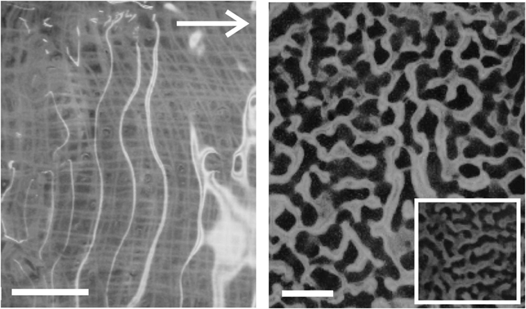
Figure 6. Examples of Kinneyia-like structures generated in the laboratory from viscoelastic films of PVA. The white arrow indicates the direction of flow for both images. Scale bars are 10 mm. Left: without any sediment added (The gauze, which was used as a substrate to graft the PVA layer, is visible through the clear film). The rippled surface is revealed by the bright reflections from the light source. Right: with a powder consisting of small (≈ 100 μm diameter) glass spheres added to mimic sedimental freight of the water flow. The inset shows some part of the sample from the outer regions of the sample where the PVA layer was thinner.

Figure 6 shows the ripples that formed in PVA films without (a) and with (b) sediment added. Increasing the flow speed appears to result in an increase in the order of the pattern, with a transition from honeycomb-like patterns to parallel ridges perpendicular to the flow direction.

The patterns generated in the “lab-Kinneyia” shown in Figure 6 qualitatively resemble the Kinneyia found in Namibia (Figure 1). Kinneyia patterns are often found to exhibit a preferred crest orientation. In Kinneyia from Öland, this orientation could be shown to run perpendicular to the paleocurrents from which the event layers were deposited (Martinsson, 1965). The results suggest that the different patterns may arise from variations in the flow conditions under which the microbial mat or film is deformed and depend upon the amount of sediment suspended in the flowing water.

Figure 7 shows the wavelength of the instability that forms as a function of the film thickness h₀. The line in Figure 7 shows a linear least-squares fit to the data with λ = 3.3h₀. This is in line with the above prediction that λ/h₀ should be between 3.2 and 4.3 (cf. Figure 5). No dependency of the wavelength on either the viscosity of the film or the flow rate was observed. This is again in agreement with the HI theory sketched above, which predicts that the wavelength only depends upon the thickness of the film. This demonstrates that the linear stability analysis yields reasonable results also for the non-linear case, i.e., when the ripple amplitude cannot be considered small as compared to the wavelength. As Figure 5D shows, the most unstable wavelength should not be strongly affected by the presence of the extra driving term from the sediment. In fact, differences in λ obtained with and without glass beads added to the flow were within experimental scattering.

FIGURE 7

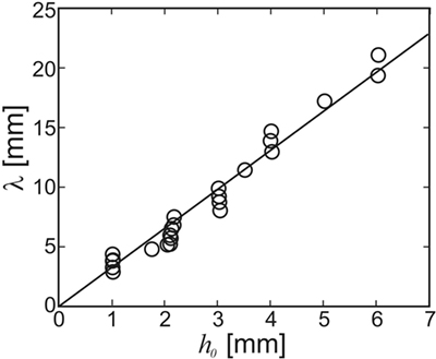
Figure 7. Wavelength of the ripple created through the hydrodynamic instability in PVA films subject to flow. The wavelength does not vary with either the flow speed or the film viscosity. The line shows a fit to the data for λ = 3.3 ± 0.3 h₀, where h₀ is the thickness of the initial PVA film [adapted with modifications from Thomas et al. (2013)].

4. Consequences and Taphonomic Suggestions

4.1. Comparison of the Models

Let us now turn to a comparative assessment of the models outlined above, as to their predictive power and consistency with findings in the fossil record. To this end, we first summarize the common features found in Kinneyia outcrops. Kinneyia ripples are found in silt layers on bedding planes in former littoral areas, with wavelengths roughly between 2 and 20 mm. The ripple profiles usually have steeper slopes than harmonic functions of the same wavelength (cf. inset of Figure 2), and their crest-to-valley height is roughly proportional to their wavelength. They can cover large areas of several square meters, or come in small patches (cf. Figure 1). They are usually found on storm wave deposits, i.e., on sedimental layers of particularly large thickness that can be attributed to storm floods.

The hydrodynamic instability (HI) model makes clear predictions about the range of wavelengths to be expected. The thickness of a MM is limited by the transport of nutrients between the different strata of the MM, i.e., from the phototrophic zone to the heterotrophic and anoxic deeper layers. Hence, it is hardly conceivable that MM ever grew substantially thicker than commonly observed in recent MM. It is, therefore, not unreasonable to assume that MM were limited to a thickness of less than a centimeter all through Earth’s history. On the other hand, a MM needs a thickness of more than the grain size of the underlying base sediment in order to form a homogeneous film. Sediments in the intertidal zones are usually sandy, i.e., with grain sizes not smaller than about 60 microns (if the standard definition of sand is applied). For a biofilm to make a continuous MM on this substrate, it needs a thickness of about a millimeter or more. If we then conclude that the thickness of a MM which will undergo the HI under flow is between 1 and 10 mm, the HI model predicts (cf. Figure 7) that the wavelength of the fossil should be at least about 3 mm, but smaller than about 30 mm. Given the crudeness of the estimate, this is remarkably close to field evidence.

Further support is gained from observations at small Kinneyia patches, such as displayed in Figure 1C. At the edges of the patch, the wavelength clearly decreases; while at the same time, the thickness of the MM must have decreased here. This is in line with the idea that the wavelength should be proportional to the MM thickness, as predicted by the HI model.

Under the assumption that the flow carried some sediment, we can also make predictions about the depth of the ripple, based on the experiments (Thomas et al., 2013). In Figure 2, the crest-to-valley amplitude of the sediment ripple generated in the experiment is plotted as the filled squares. Clearly, the depth is very well comparable to the depth of the Kinneyia ripples found in the outcropping fossils, not only in its roughly linear variation with the wavelength but also in its absolute value. Hence, we find that all of the obvious features of Kinneyia are in agreement with the HI model.

As far as the oscillating flow (OF) model is concerned, we first note that the patterns obtained in the experimental setting (cf. inset in Figure 3B) are of striking similarity with the Kinneyia fossil, just as those found for the HI experiments. Furthermore, the wavelength is of the right order of magnitude. However, we have already seen that the range of wavelengths is only correctly predicted if the depth of the water is between 9 and 15 cm (cross-hatched region in Figure 4). Moreover, in order to fulfill the experimental conditions under which the ripples formed, the amplitude of the sloshing flow is required to be constant for as long as 24 h. While such conditions may occasionally occur, they can certainly not be considered generic. Finally, we note that a local variation of the wavelength as strong as seen in Figure 1C is not readily explained by this model.

This may be better accounted for by the liquefied sediment (LS) model, where a patchy appearance as shown in Figure 1C is readily explained by local variations of microbial density (and hence metabolic activity) in the underlying sediment. We should note, however, that the LS model requires a number of very specific criteria to be met, and makes no clear prediction concerning the wavelength and topography of the ripple. Hence, it can as yet not be quantitatively compared with the other models concerning its agreement (or disagreement) with observations.

We, thus, find that the HI model accounts very well, in all of its predictions, for the characteristics found in Kinneyia fossils. Agreement with the predictions of the OF model may occur, but is linked to some rather special conditions. The LF sediment model does not make predictions quantitative enough to decide on its relevance in the formation of Kinneyia. As a result, we conclude that the mechanism of the HI is very probably of greatest relevance in the formation of Kinneyia. The other two mechanisms cannot be ruled out to play a role occasionally, but this needs extra information in order to be clearly decided.

4.2. Taphonomic Consequences

Having thus arrived at a certain preference of the HI model, we should compare its predictions in some more detail with the fossil record. The upper layer of the storm wave deposits, where Kinneyia is found is frequently observed to be covered with a thin topset veneer thought to have sedimented after the event deposit at shallow water depths. Thin sections made from Kinneyia from Öland, Sweden (Porada et al., 2008) show that the depth of the veneer is proportional to the amplitude of the ripple structure, with the bottom of the veneer layer sometimes coinciding with the troughs of the Kinneyia.

It is easy to see that this structure is readily formed in a process dominated by the HI mechanism. When the amplitude of the ripple reaches a certain threshold, eddies will form in the valleys of the undulation (Figure 5C). Some of the clastic sediments carried by the overlying fluid as it flows will settle in the troughs due to the back flow and stagnation points arising from the eddies. The growth of the ripple pattern is thereby accelerated and steep slopes develop between the troughs and the crests. As the microbial mat dies, remains of the EPS glue the sediments together, preserving the Kinneyia structures that are found in the geologic record.

Figure 8 shows two sequences of formation of sedimentary ripples from the HI, for small amounts of sediment Figures 8A–C and for large amounts of sediment Figures 8D–F. The sedimentary pattern which will finally form the fossil structure is shown in Figures 8C,F, respectively. For the step from Figures 8E,F, note that the microbial material is expected to dry away and decay, such that the top layer of sediment will sink to the bedding plane by gravity, while more or less conserving its local thickness. It may do so already before, after the flow has stopped, through the large specific weight of the sediment and the ductile consistency of the MM. Obviously, it is easily conceivable to have structures with both exposed bedding plane (Figure 8C) and with a thin veneer layer still present above the bedding plane (Figure 8F). In any case, the bottom of the ripple will be close to the bedding plane, similar to what is observed in Kinneyia fossils (Porada et al., 2008).

FIGURE 8

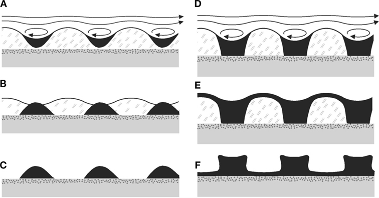
Figure 8. Possible taphonomic sequences leading to Kinneyia fossils. (A–C) Sediment accumulates in the troughs of the ripple forming in the MM, and subsequently sinks down to the bedding plane due to gravity (B). When the mat disintegrates, crests of sediment are left, which can fossilize subsequently. (D–F) Same mechanism as before, but with more sediment being deposited. As a consequence, there may finally (F) be connected crests, and various shapes of the slopes are conceivable.

5. The Decreasing Occurrence of Kinneyia after the Paleozoic

The robustness of the HI mechanism suggests that Kinneyia-type structures should be found not only in the fossil record but also abundantly in modern biomats. However, wrinkle patterns are only very occasionally observed in modern biomats and generally have morphologies that differ from Kinneyia patterns. Furthermore, it has been repeatedly noted that Kinneyia gradually vanishes from the fossil record during the Mesozoic. Some are found up to the Jurassic, such as the one found very recently in Sweden near Helsingborg (Peterffy et al., 2016), but newer instances are extremely rare. Although some authors claim that this may be due to a bias in observation (Davies et al., 2016), the scarcity of reports of Kinneyia after the Jurassic is striking. Hence, the universal applicability of the HI mechanism to MM may in fact constitute a problem, as this calls for an explanation of the absence of Kinneyia-type ripples in both modern MM and post-Mesozoic sediments from former littoral areas.

One possible reason for the gradual decrease of Kinneyia in the fossil record, since the Cambrian, is that MM have become less ubiquitous, due to grazing and bioturbation (Hagadorn and Bottjer, 1997; Schieber, 2007; Peterffy et al., 2016). However, this does not fully explain, especially in light of the universal character of the HI mechanism, the scarcity of Kinneyia-type ripples, even in modern mats. One might, of course, argue that modern MM usually occur in protected, sheltered, and frequently hypersaline areas with low hydrodynamic activity, where storms are not likely to occur. But then one would need to maintain that this must have been the case all throughout the Phanerozoic, while Kinneyia gradually disappeared. Clearly, this is not very satisfactory.

5.1. Possible Memory Effects in Viscoelastic Films

A speculative, but very interesting, line of thought concerns the rheological properties of biomats. Although modern biofilms may appear to be viscoelastic media to a rheometer, we know that active mechano-response is well conserved at least in modern eucaryotes. Strictly speaking, biomats should, therefore, be viewed as active matter, such that their response to a superficial flow may be more complex than that of a passive viscoelastic material. As we do not know the history of mechano-response evolution, the mechanical properties of biomats may have been, subtly but distinctly, different when Kinneyia fossils formed.

The breakup of a MM as depicted in Figure 8 is expected to kill the MM since it destroys its stratigraphic organization. It is, therefore, interesting to investigate whether MM might have developed strategies to sidestep the HI mechanism altogether. One possibility to achieve this could be to develop an active mechanical response that changes the dynamics of the MM interface under flow, such as to remove the HI. This leads to the interesting question of whether the evolution of mechano-response of cells might have in part been due to the evolutionary pressure on MM to evade the HI in flowing water environments. Let us, thus, discuss possible consequences of an active response, in particular of the kind observed in cells living today.

The HI of a microbial mat boils down to a simple first-order differential equation in the time domain [cf. equation (9)]:

${\partial }_t{\mathrm{\epsilon }}_0=\mathrm{\alpha }\left(q\right){\mathrm{\epsilon }}_0$ (11)

where ε₀(t) is the amplitude of a sinusoidal small perturbation with wave number q. α is a growth constant which is positive for unstable modes. Equation (11) is derived for a purely passive viscous or viscoelastic film. The question we want to discuss here is whether any kind of “active” response of the film material to the applied stress can stall the instability even for positive α.

If cells, such as those of which the biomat is composed, respond antagonistically to an applied stress, with a certain delay corresponding to the rearrangement of cytoskeletal matter, we expect an additional term of the form

${\displaystyle \underset{0}{\overset{t}{\int }}}R\left(\mathrm{\tau }\right){\dot{\mathrm{\epsilon }}}_0\left(t-\mathrm{\tau }\right)d\mathrm{\tau }$ (12)

to appear in equation (11), where R(τ) is the stress response after delay τ. The time derivative $\dot{\mathrm{\epsilon }}$₀ = ∂_tε₀ enters because the cells are stressed only while the mat is being deformed, and according to the rate at which this happens. Inserting equation (12) in equation (11) yields then

${\partial }_t{\mathrm{\epsilon }}_0=\mathrm{\alpha }\left(q\right){\mathrm{\epsilon }}_0+\mathrm{\varrho }{\displaystyle \underset{0}{\overset{t}{\int }}}R\left(\mathrm{\tau }\right){\dot{\mathrm{\epsilon }}}_0\left(t-\mathrm{\tau }\right)d\mathrm{\tau }.$ (13)

where ϱ determines the strength of the active response. This equation is of a similar form as the equation of motion of correlations in ideal glass forming models, called mode-coupling equation. It is known that the occurrence of a memory term, such as the integral expression in equation (13), may indeed stall the dynamics of its solutions (ε, in our case), for a wide range of memory kernels, R(τ) (Götze and Voigtmann, 2000).

R(τ) should qualitatively look as sketched in the inset in Figure 9. Its support is limited to the positive τ axis because of causality. The area under the curve shall be normalized to unity. Since the reaction is assumed to be antagonistic, in accordance with common observations of cell mechanics, we assume ϱ < 0.

FIGURE 9

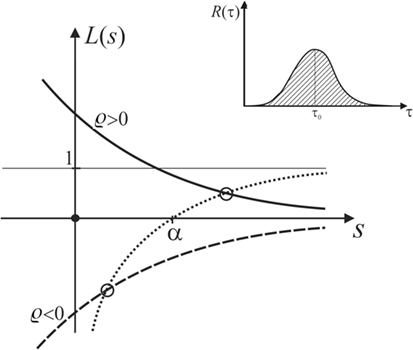
Figure 9. Plot of L(s), showing that the latter always intersects the function $\text{1}-\frac{\mathrm{\alpha }}{s}$ in the domain of positive s if α is positive.

Now let us apply the Laplace transform to equation (13). We obtain

$s{\widehat{\mathrm{\epsilon }}}_0\left(s\right)-{\mathrm{\epsilon }}_0\left(0\right)=\mathrm{\alpha }{\widehat{\mathrm{\epsilon }}}_0\left(s\right)+\mathrm{\varrho }\left(s{\widehat{\mathrm{\epsilon }}}_0\left(s\right)-{\mathrm{\epsilon }}_0\left(0\right)\right)\widehat{R}$ (14)

where

${\widehat{\mathrm{\epsilon }}}_0\left(s\right)={\displaystyle \underset{0}{\overset{\infty }{\int }}}{\mathrm{\epsilon }}_0\left(t\right)e^{-\mathit{st}}\mathit{dt}$ (15)

and $\widehat{R}$ are the Laplace transforms of ε₀ and the response function, respectively. Rearranging equation (14) and setting $L\left(s\right)=\mathrm{\varrho }\widehat{R}$, we obtain

${\widehat{\mathrm{\epsilon }}}_0\left(s\right)\propto \frac{1-L}{s\left(1-L\right)-\mathrm{\alpha }},$ (16)

which has a pole at some s_p, with s_p(1 − L(s_p)) = α, or

$L\left(s_p\right)=1-\frac{\mathrm{\alpha }}{s_p}$ (17)

which is sketched as the dotted curve in Figure 9.

Let us now discuss any general R(τ) that looks qualitatively as sketched in the inset of Figure 9. It is obvious that $\widehat{R}$ will always be monotonic and decay to zero as s becomes larger than 1/τ₀, but approaches unity for small s. For positive or negative ϱ, this leads to the solid or dashed curve, respectively, representing the graph of L(s) in Figure 9.

The growth rate of the displacement of the MM interface, which corresponds to the pole of ${\widehat{\mathrm{\epsilon }}}_0\left(s\right)$, is determined by seeking the intersection the graph of L(s) with the graph of $1-\frac{\mathrm{\alpha }}{s}$. As demonstrated in Figure 9, these intersections always lie in the domain of positive s if α is positive, no matter if ϱ < 0 or ϱ > 0.

Hence, we conclude that any active response entering the equation of motion like equation (13), with R(τ) positive, normalized and real, will change the rate of growth of the ripple amplitude, but never stall the instability. Note that this discussion considers active bulk response only. Active surface motility in response to flow [rheotaxis (Dalous et al., 2008; Lima et al., 2014)] may behave differently, but needs to be further investigated. With this caveat in mind, we may so far conclude that active mechanic response, as observed widely in living cells today, has very probably not evolved in ancient MM in an effort to evade the HI instability leading to Kinneyia ripples.

5.2. Lessons from Storm Wave Deposits

An aspect we have not addressed so far is that Kinneyia is most frequently found on particularly thick layers of sediment, deposited in large-scale storm flood events. The Haruchas outcrop (Figure 1C), for instance, sits in a modern dry river bed, with Kinneyia on top of a siltstone layer as thick as about 20 cm, which is much thicker than the adjacent strata as far as they are visible in the outcrop. In case of the Neuras outcrop (Figures 1A,B), the event deposit on which the Kinneyia were observed was ~35-cm thick. The correlation with storm wave deposits calls for explanation, and may result in more valuable hints as to its mechanism of generation.

Recall that during the times of formation of the Kinneyia fossils from Figure 1, which lies in the Precambrian, there were neither plants on the land masses nor burrowing animals that could have caused bioturbation of any kind to the predominantly flat sedimental deposits in most littoral areas (Figure 10A). Hence, the topographic conditions for Kinneyia formation were favorable, but we need to understand what conditions may have led to the growth of MM and to the formations of ripples in them. We will see that storm flood events provide a quite natural basis for this both to happen.

FIGURE 10

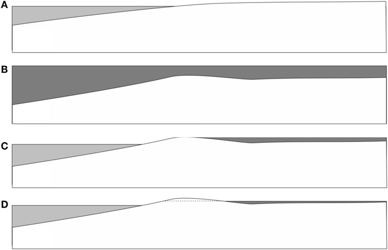
Figure 10. Possible scenario for flooding of a littoral area during a storm event. (A) Before the event. (B) During the storm, wide areas are flooded with water carrying large amounts of sediment and microbes (dark gray) from the sea floor areas. A shallow barrier of accumulated sediment emerges. (C) After the event, the flooded areas remain covered with extended lagoons, due to sediment barriers close to the shore. Microbes have time to settle down and form thick films on the bedding plane. (D) As the flood drains through gaps in the sedimental barrier, the water moves with an increasing flow velocity. As this reaches appreciable values, the hydrodynamic instability sets in, forming Kinneyia ripples.

Let us imagine a few common features of storm flood events. First of all, the water level rises by up to several meters, and the land close to the shore is being flooded by waters carrying a large amount of sediment, which is stirred up from the littoral range of the sea floor (Figure 10B). As a consequence, large amounts of the heavier fractions of the sediment (sand and gravel) are deposited close to the shore line. These deposits form barriers that prevent parts of the water flooding the land from flowing back into the sea after the storm (Figure 10C). As a consequence, the land close to the seashore, up to many kilometers inland, may remain flooded for weeks after the storm has ceased. During that time, the lighter sedimental fractions will settle out of the seawater onto the flat land bedding. Among these lighter fractions, there are in particular the microbes that had populated the littoral sea floor areas, and which had been stirred up along with the mineral sediment. If there is enough biological material, biofilms will be necessarily created on the flooded land just by sedimentation. If these find sufficiently favorable conditions (such as enough light penetrating through the water layer), MM mats are easily formed. They may cover enormous areas within the flooded zone.

Now we consider how the water drains back into the sea (Figure 10D). This will happen through crevasses in the barrier deposits. The volumetric flow rate through these crevasses is limited (and, therefore, largely determined) by their size. If then the height of the flood is H, the flow velocity V at which the flood recedes back into the sea scales as V ∝ 1/H, with the flow rate through the crevasses determining the prefactor. Hence, there will be almost no perceivable flow velocity for an extended period of time after the flood, but it will build up to considerable velocities (up to typical tidal current flow of order meters per second) as the flood comes close to its end (H → 0).

As a consequence, a storm flood provides a perfect scenario for Kinneyia ripples to form through the HI model. First, there is an extended time during which microbes settle on the ground in large amounts, possibly forming cohesive MM if the layer is not too thick (for enabling nutrient transport, etc.). Then, but only after some delay, there will be a flow velocity building up which (as we have seen from the reported experiments) leads almost inevitably to a HI forming Kinneyia-like ripples.

This scenario provides an additional possible explanation why Kinneyia seems to vanish gradually from the fossil record after the Cambrian radiation. Not only grazing animals were impeding its generation, but also plants, roots, burrowing, and other aspects of bioturbation destroyed the flat plains on which Kinneyia would have formerly formed quite naturally after a storm. Hence, the scenario put forward above would underscore the common idea that the increasing presence of higher life forms have impeded the formation of Kinneyia through MM (Peterffy et al., 2016). Here, we just add bioturbation and plant cover as an alternative (or additional pathway) to grazing.

6. Conclusion

In conclusion, we reviewed several possible mechanisms that might lead to ripple structures in sedimental layers, showing up in the fossil record as the so-called Kinneyia. We have identified a hydrodynamic instability due to water flowing over a microbial mat as a particularly probable mechanism at the basis of Kinneyia formation. Although a role for the other mechanisms considered cannot be completely ruled out, they are lacking either quantitative predictions (as the liquefied sediment model, which would need further elaboration) or agreement of the predicted wavelengths with field evidence (as for the oscillating flow model) to thoroughly judge their relevance. The hydrodynamic instability model, by contrast, does not only correctly predict the observed range of wavelengths but it also agrees with Kinneyia fossils in terms of the scaling of the ripple depth with the wavelength, as well as with the overall appearance. Furthermore, we have seen that if the HI is indeed the dominant mechanism, storm events are expected to be particularly well suited to produce Kinneyia ripples. This is well in line with the noticeable correlation of Kinneyia outcrops with storm wave deposits. It furthermore provides a natural explanation of the gradual disappearance of Kinneyia from the fossil record during the Mesozoic. The increasing abundance of animals and plants did not only lead to decimation of MM by grazing but also to bioturbation of the formerly flat areas where Kinneyia would form naturally after a storm event. On a substrate that is strongly disturbed by roots and burrowing animals, this is not readily possible.

Author Contributions

SH conceived the paper and elaborated the theory. SH, LG, HP, and KT wrote the paper. KT, LG, SH, and SA performed experiments.

Conflict of Interest Statement

The authors declare that the research was conducted in the absence of any commercial or financial relationships that could be construed as a potential conflict of interest.

Acknowledgments

We thank the team of the Göttingen Culture Collection of Algae (http://www.uni-goettingen.de/en/45175.html) for numerous helpful hints and access to their algae cultures. We express our special gratitude to our colleague El Hafid Bouougri for valuable comments and critical reading of the manuscript.

Footnote

1. ^In Thomas et al. (2013), it has been assumed that this process leads to P(q) ∝ 1∕q, which appears less well justified.

References

Allen, J. R. L. (1966). A beach structure due to wind-driven foam. J. Sediment. Petrol. 37, 691–692. doi: 10.1306/74D71758-2B21-11D7-8648000102C1865D

CrossRef Full Text | Google Scholar

Allwood, A. C., Walter, M. R., Kamber, B. S., Marshall, C. P., and Burch, I. W. (2006). Stromatolite reef from the early Archaean era of Australia. Nature 441, 714–718. doi:10.1038/nature04764

CrossRef Full Text | Google Scholar

Bergdahl, L. (2009). “Comparison of measured shallow-water wave spectra with theoretical spectra,” in Proceedings of the 8th European Wave and Tidal Energy Conference. Uppsala, Sweden, 100–105.

Google Scholar

Bordner, G. L. (1978). Nonlinear analysis of laminar boundary layer flow over a periodic wavy surface. Phys. Fluids 21, 8581471. doi:10.1063/1.862409

CrossRef Full Text | Google Scholar

Bouougri, E. H., and Porada, H. (2007). Siliciclastic biolaminites indicative of widespread microbial mats in the Neoproterozoic Nama Group of Namibia. J. Afr. Earth Sci. 48, 38. doi:10.1016/j.jafrearsci.2007.03.004

CrossRef Full Text | Google Scholar

Casanova, J., Jose, J., Garcia-Berro, E., Shore, S. N., and Calder, A. C. (2011). Kelvin-Helmholtz instabilities as the source of inhomogeneous mixing in nova explosions. Nature 478, 490–492. doi:10.1038/nature10520

CrossRef Full Text | Google Scholar

Dalin, P., Pertsev, N., Frandsen, S., Hansen, O., Andersen, H., Dubietis, A., et al. (2010). A case study of the evolution of a Kelvin-Helmholtz wave and turbulence in noctilucent clouds. J. Atmos. Sol. Terr. Phys. 72, 1129–1138. doi:10.1016/j.astp.2010.06.011

CrossRef Full Text | Google Scholar

Dalous, J., Burghardt, E., Müller-Taubenberger, A., Bruckert, F., Gerisch, G., and Bretschneider, T. (2008). Reversal of cell polarity and actin-myosin cytoskeleton reorganization under mechanical and chemical stimulation. Biophys. J. 94, 1063–1074. doi:10.1529/biophysj.107.114702

CrossRef Full Text | Google Scholar

Davies, N. S., Liu, A. G., Gibling, M. R., and Miller, R. F. (2016). Resolving MISS conceptions and misconceptions: a geological approach to sedimentary surface textures generated by microbial and abiotic processes. Earth Sci. Rev. 154, 210–246. doi:10.1016/j.earscirev.2016.01.005

CrossRef Full Text | Google Scholar

de Brouwer, J. F. C., Wolfstein, K., Ruddy, G. K., Jones, T. E. R., and Stal, L. J. (2005). Biogenic stabilization of intertidal sediments: the importance of extracellular polymeric substances produced by benthic diatoms. Microb. Ecol. 49, 501–512. doi:10.1007/s00248-004-0020-z

CrossRef Full Text | Google Scholar

Donlan, R. M. (2002). Biofilms: microbial life on surfaces. Emerg. Infect. Dis. 8, 881–890. doi:10.3201/eid0809.020063

CrossRef Full Text | Google Scholar

Dupraz, C., Visscher, P. T., Baumgartner, L. K., and Reid, R. P. (2004). Microbe-mineral interactions: early carbonate precipitation in a hypersaline lake (Eleuthera Island, Bahamas). Sedimentology 51, 745–765. doi:10.1111/j.1365-3091.2004.00649.x

CrossRef Full Text | Google Scholar

Flemming, H. C., and Wingender, J. (2010). The biofilm matrix. Nat. Rev. Microbiol. 8, 623–633. doi:10.1038/nrmicro2415

CrossRef Full Text | Google Scholar

Friedmann, E. I., and Weed, R. (1987). Microbial trace-fossil formation, biogenous, and abiotic weathering in the Antarctic cold desert. Science 236, 703–705. doi:10.1126/science.11536571

CrossRef Full Text | Google Scholar

Gerdes, G. (2007). “Structures left by modern microbial mats in their host sediments,” in Atlas of Microbial Mat Features Preserved within the Clastic Rock Record, eds J. Schieber, P. K. Bose, P. G. Eriksson, S. Banjeree, S. Sarkar, W. Altermann, and O. Catuneau (Amsterdam: Elsevier), 5–38.

Google Scholar

Gerdes, G., Klenke, T., and Noffke, N. (2000). Microbial signatures in peritidal siliciclastic sediments: a catalogue. Sedimentology 470, 279–308. doi:10.1046/j.1365-3091.2000.00284.x

CrossRef Full Text | Google Scholar

Götze, W., and Voigtmann, T. (2000). Universal and nonuniversal features of glassy relaxation in propylene carbonate. Phys. Rev. E 61, 4133. doi:10.1103/PhysRevE.61.4133

CrossRef Full Text | Google Scholar

Hagadorn, J. W., and Bottjer, D. J. (1997). Wrinkle structures: microbially mediated sedimentary structures common in subtidal siliciclastic settings at the Proterozoic-Phanerozoic transition. Geology 25, 1047–1050. doi:10.1130/0091-7613(1997)025<1047:WSMMSS>2.3.CO;2

CrossRef Full Text | Google Scholar

Hagadorn, J. W., and Bottjer, D. J. (1999). Restriction of a late Neoproterozoic biotope: suspect-microbial structures and trace fossils at the Vendian-Cambrian transition. Palaios 14, 73–85. doi:10.2307/3515362

CrossRef Full Text | Google Scholar

Hall-Stoodley, L., and Stoodley, P. (2009). Evolving concepts in biofilm infections. Cell. Microbiol. 11, 1034–1043. doi:10.1111/j.1462-5822.2009.01323.x

CrossRef Full Text | Google Scholar

Hasegawa, H., Fujimoto, M., Pan, T. D., Reme, H., Boalogh, A., Dunlop, M. W., et al. (2004). Transport of solar wind into earth’s magnetopshere through rolled up Kelvin-Hemholtz vortices. Nature 430, 755–758. doi:10.1038/nature02799

CrossRef Full Text | Google Scholar

Hawes, I., Summer, D. Y., Andersen, D. T., Jungblut, A. D., and Mackey, T. J. (2013). Timescales of growth response of microbial mats to environmental change in an ice-covered Antarctic lake. Biology (Basel) 2, 151–176. doi:10.3390/biology2010151

CrossRef Full Text | Google Scholar

Landau, L. D., and Lifshitz, E. M. (1959). Fluid Mechanics (Course of Theoretical Physics), Volume 6. Oxford: Pergamon Press.

Google Scholar

Lieleg, O., Caldara, M., Baumgaertel, R., and Ribbeck, K. (2011). Mechanical robustness of Pseudomonas aeruginosa biofilms. Soft Matter 7, 3307–3314. doi:10.1039/c0sm01467b

CrossRef Full Text | Google Scholar

Lima, W. C., Vinet, A., Pieters, J., and Cosson, P. (2014). Role of PKD2 in rheotaxis in Dictyostelium. PLoS ONE 9:e88682. doi:10.1371/journal.pone.0088682

CrossRef Full Text | Google Scholar

Liu, P. (1985). Representing frequency spectra for shallow water waves. Ocean Eng. 12, 151–160. doi:10.1016/0029-8018(85)90078-2

CrossRef Full Text | Google Scholar

Mariotti, G., Pruss, S. B., Perron, J. T., and Bosak, T. (2014). Microbial shaping of sedimentary wrinkle structures. Nat. Geosci. 7, 736–740. doi:10.1038/ngeo2229

CrossRef Full Text | Google Scholar

Martinsson, A. (1965). Aspects of middle Cambrian thanatotope on Öland. Geol. Foeren. Stockholm Foerh. 87, 181–230. doi:10.1080/11035896509448903

CrossRef Full Text | Google Scholar

Mayer, C., Moritz, R., Kirschner, C., Borchard, W., Maibaum, R., Wingender, J., et al. (1999). The role of intermolecular interactions: studies on model systems for bacterial biofilms. Int. J. Biol. Macromol. 26, 3–16. doi:10.1016/S0141-8130(99)00057-4

CrossRef Full Text | Google Scholar

Miche, R. (1951). Reflectivity of marine structures exposed to action of waves. Ann. des Ponts et Chaussees, 121, 285–319.

Google Scholar

Neu, T. R., and Lawrence, J. R. (1997). Development and structure of microbial biofilms in river water studied by confocal laser scanning microscopy. FEMS Microbiol. Ecol. 24, 11–25. doi:10.1111/j.1574-6941.1997.tb00419.x

CrossRef Full Text | Google Scholar

Noffke, N. (2010). Geobiology: Microbial Mats in Sandy Deposits from the Archean Era to Today. Berlin, Heidelberg: Springer-Verlag.

Google Scholar

Noffke, N., Gerdes, G., and Klenke, T. (2003a). Benthic cyanobacteria and their influence on the sedimentary dynamics of peritidal depositional systems (siliciclastic, evaporitic salty, and evaporitic carbonatic). Earth Sci. Rev. 62, 163–176. doi:10.1016/S0012-8252(02)00158-7

CrossRef Full Text | Google Scholar

Noffke, N., Knoll, A. H., and Grotzinger, J. P. (2002). Sedimentary controls on the formation and preservation of microbial mats in siliciclastic deposits: a case study from the Upper Neoproterozoic Nama Group, Namibia. Palaios 17, 533–544. doi:10.1669/0883-1351(2002)017<0533:SCOTFA>2.0.CO;2

CrossRef Full Text | Google Scholar

Peterffy, O., Calnera, M., and Vajda, V. (2016). Early Jurassic microbial mats – a potential response to reduced biotic activity in the aftermath of the end-Triassic mass extinction event. Palaeogeogr. Palaeoclimatol. Palaeoecol. doi:10.1016/j.palaeo.2015.12.024

CrossRef Full Text | Google Scholar

Pfluger, F. (1999). Matground structures and redox facies. Palaios 14, 25–39. doi:10.2307/3515359

CrossRef Full Text | Google Scholar

Pfluger, F., and Gresse, P. G. (1996). Microbial sand chips – a non-actualistic sedimentary structure. Sediment. Geol. 102, 263–274. doi:10.1016/0037-0738(95)00072-0

CrossRef Full Text | Google Scholar

Porada, H., and Bouougri, E. H. (2007). Wrinkle structures – a critical review. Earth Sci. Rev. 81, 199–215. doi:10.1016/j.earscirev.2006.12.001

CrossRef Full Text | Google Scholar

Porada, H., Ghergut, J., and Bouougri, E. H. (2008). Kinneyia-type wrinkle structures – critical review and model of formation. Palaios 23, 65–77. doi:10.2110/palo.2006.p06-095r

CrossRef Full Text | Google Scholar

Rupp, C. J., Fux, C. A., and Stoodley, P. (2005). Viscoelasticity of Staphylococcus aureus biofilms in response to fluid shear allows resistance to detachment and facilitates rolling migration. Appl. Environ. Microbiol. 71, 2175–2178. doi:10.1128/AEM.71.4.2175-2178.2005

CrossRef Full Text | Google Scholar

Sarkar, S., Bose, P. K., Samanta, P., Sengupta, P., and Eriksson, P. G. (2008). Microbial mat mediated structures in the Ediacaran Sonia Sandstone, Rajasthan, India and their implications from Proterozoic sedimentation. Precambrian. Res. 162, 248–263. doi:10.1016/j.precamres.2007.07.019

CrossRef Full Text | Google Scholar

Schieber, J. (2007). “Microbial mats on muddy substrates – examples of possible sedimentary features and underlying processes,” in Atlas of Microbial Mat Features Preserved within the Siliciclastic Rock Record, eds J. Schieber, P. K. Bose, P. G. Eriksson, S. Banjeree, S. Sarkar, W. Altermann, and O. Catuneau (Amsterdam: Elsevier).

Google Scholar

Schieber, J., Bose, P. K., Eriksson, P. G., Banerjee, S., Sarkar, S., Altermann, W., (eds) (2007). Atlas of Microbial Mat Features Preserved within the Siliciclastic Rock Record. Amsterdam: Elsevier.

Google Scholar

Schieber, J., and Glamoclija, M. (2007). “Microbial mats built by iron bacteria: a modern example from southern Indiana,” in Atlas of Microbial Mat Features Preserved within the Siliciclastic Rock Record, eds J. Schieber, P. K. Bose, P. G. Eriksson, S. Banjeree, S. Sarkar, W. Altermann, and O. Catuneau (Amsterdam: Elsevier).

Google Scholar

Scholle, M., Haas, A., Aksel, N., Wilson, M. C., Thompson, H. M., and Gaskell, P. H. (2008). Competing geometric and inertial effects on local flow structure in thick gravity-driven fluid films. Phys. Fluids 20, 123101. doi:10.1063/1.3041150

CrossRef Full Text | Google Scholar

Shaw, T., Winston, M., Rupp, C. J., Klapper, I., and Stoodley, P. (2004). Commonality of elastic relaxation times in biofilms. Phys. Rev. Lett. 93, 098102. doi:10.1103/PhysRevLett.93.098102

CrossRef Full Text | Google Scholar

Shrock, R. R. (1948). Sequence in Layered Rocks. New York: McGraw Hill.

Google Scholar

Singh, I. B., and Wunderlich, F. (1978). On the terms wrinkle marks (runzelmarken), millimeter ripples and mini ripples. Senckenb. Marit. 10, 75–83.

Google Scholar

Smyth, W. D., and Moum, J. N. (2012). Ocean-mixing by Kelvin-Hemholtz instability. Oceanography 25, 140–149. doi:10.5670/oceanog.2012.49

CrossRef Full Text | Google Scholar

Thomas, K., Herminghaus, S., Porada, H., and Goehring, L. (2013). Formation of Kinneyia via shear-induced instabilities in microbial mats. Phil. Trans. R. Soc. A 371, 20120362. doi:10.1098/rsta.2012.0362

CrossRef Full Text | Google Scholar

Verstrepen, K. J., and Klis, F. M. (2006). Flocculation, adhesion and biofilm formation in yeasts. Mol. Microbiol. 60, 5–15. doi:10.1111/j.1365-2958.2006.05072.x

CrossRef Full Text | Google Scholar

Vinogradov, A. M., Winston, M., Rupp, C. J., and Stoodley, P. (2004). Rheology of biofilms formed from the dental plaque pathogen Streptococcus mutans. Biofilms 1, 49–56. doi:10.1017/S1479050503001078

CrossRef Full Text | Google Scholar

Wingender, J., Neu, T. R., and Flemming, H. C. (eds) (1999). Microbial Extracellular Polymeric Substances. Berlin, Heidelberg: Springer-Verlag.

Google Scholar

Wolff, T. (1977). Diversity and faunal composition of the deep-sea benthos. Nature 267, 780–785. doi:10.1038/267780a0

CrossRef Full Text | Google Scholar

Zolghadr, B., Klingl, A., Koerdt, A., Driessen, A. J. M., Rachel, R., and Albers, S. V. (2010). Appendage-mediated surface adherence of Sulfolobus solfataricus. J. Bacteriol. 192, 104–110. doi:10.1128/JB.01061-09

CrossRef Full Text | Google Scholar