A signal processing analysis of Purkinje cells in vitro

Introduction

The Purkinje Cell (PC) in the cerebellum is a perpetually firing cell, with a high degree of basal activity shaping its output to the deep cerebellar nuclei. The output of the PC is modulated by both excitatory and inhibitory connections via its pronounced dendritic arborization (Ito, 2006 , 2001 ). Various computational functions have been attributed to the PC due to its conspicuous network geometry, including interpretations based on the classical perceptron model (Marr, 1969 ; Albus, 1971 ), feedback circuit models (Doya et al., 2001 ; Sklavos et al., 2005 ; Ito, 2006 ) and those involving temporal oscillations (Cheron et al., 2008 ; De Zeeuw et al., 2008 ; Jacobson et al., 2008 ). Evidence of long term depression in the Purkinje-parallel fiber synapses (Ekerot and Kano, 1985 ; Kano and Kato, 1987 ) and of temporal patterns in the output signal (Jaeger and Bower, 1994 ; Lang et al., 1999 ; Shin et al., 2007 ; Steuber et al., 2007 ) have reinforced these interpretations, and functional computer models of the PC have been created using experimental data to recreate many of the known characteristics of PCs (De Schutter and Bower, 1994 ; Achard and De Schutter, 2008 ).

Prevalent interpretations of PC signal output have focused on either the pauses in the output signal (Jaeger and Bower, 1994 ; Steuber et al., 2007 ), or on the bistable nature of the cell, where the PC exists either in a depolarized state of firing, or quiescence (Chang et al., 1993 ; Womack and Khodakhah, 2002 ; Loewenstein et al., 2005 ; McKay et al., 2007 ). The existence of bistability in in vitro, and anesthetized in vivo preparations has been recently assumed to be an artifact of the anesthetic used in in vivo studies (Schonewille et al., 2005 ). While there is evidence implicating external input control of bistable transitions, specifically the climbing fiber (Loewenstein et al., 2005 ; McKay et al., 2007 ; Davie et al., 2008 ), there is a general disagreement over whether such recurrences are stochastic (Keating and Thach, 1997 ; Kitazawa and Wolpert, 2005 ; Hakimian et al., 2008 ) or periodic (Llinás and Sugimori, 1980 ; Chang et al., 1993 ).

Signal processing techniques lie at the foundation of information theory and describe the coding of neural signals from a more holistic standpoint (Roberts, 1979 ; Bialek et al., 1991 ). For a continuously firing cell such as the PC, there are distinct advantages to interpreting the signal output using tools from signal processing. Variations on the Fourier transform (Fast-Fourier Transform, FFT) can detect hidden recurrent frequencies in a signal, allowing the decomposition of a signal into its fundamental modes, and can track these modes over time (Oppenheim and Willsky, 1983 ). The PC output is particularly amenable to analysis using techniques such as FFTs since its firing patterns are long, continuous, and replete with recurring patterns (Shin et al., 2007 ; Steuber et al., 2007 ).

By describing the PC output in terms of its frequencies, we devise a model description of the PC output as a combination of three frequencies that are inherent to the PC. The three frequencies consist of Na⁺ spikes (hereby referred to as the “Sodium” or Carrier frequency), Ca²⁺ spikes (hereby the “Calcium” or Envelope frequency), and a here-defined “Switching” frequency (named such that it “switches” the firing rate from quiescence to firing). A detailed analysis of the Calcium and Switching frequencies is given, with a distribution of the Ca²⁺ spikes in the PC being in the range of ∼1–15 Hz, and Switching frequencies occurring below 1 Hz. Combining these frequencies using simple signal processing equations effectively recreates many of the known waveforms seen in PC recordings. This form of signal decomposition leads to an interpretation of the PC signal output that can describe the seemingly “random” distribution of pauses in the neural code (Keating and Thach, 1997 ; Kitazawa and Wolpert, 2005 ). Finally, using a unique photo-switchable kainate receptor agonist (Volgraf et al., 2007 ), we demonstrate the ability to modulate the frequency of the Ca²⁺ spikes in a PC using an optical stimulation input.

Materials and Methods

Animals

Animal handling and care was done according to guidelines set by the Office of Laboratory Animal Care (OLAC) at UC Berkeley. Sprague-Dawley rats (aged 21–30) were initially euthanized using isoflurane and then decapitated. Their cerebella were isolated and 250-µM thick parasagittal slices were obtained using a vibratome (Leica, VT1000s) while submerged in a sucrose-based slicing media (see Solutions). Brain slices were transferred to an incubation chamber containing ACSF bubbled with carboxygen (95%O₂/5%CO₂) held at 37°C for 1–4 h.

Solutions

Artificial Cerebro-Spinal Fluid (ACSF) containing 125 mM NaCl, 2.5 mM KCl, 1.25 mM NaH₂PO₄, 2 mM CaCl₂, 1 mM MgCl₂, 25 mM glucose and 26 mM NaHCO₃ (pH ∼7.3, 306 osm) was used for all experiments. A sucrose-based slicing media was prepared as a modified ACSF by substituting the NaCl with iso-osmolar sucrose. Internal solutions were composed of 68 mM K-gluconate, 68 mM KCl, 0.2 mM EGTA, 2 mM MgSO₄, 20 mM HEPES, 2 mM Na₂ATP and 0.5 mM Na₂GTP, along with 30 µM of Alexa 488 dye.

Measurements

All experiments were done in a closed-loop, heated perfusion chamber (34 ± 1°C). The closed-loop system allowed the recycling of solutions, when desired, using a pair of peristaltic pumps. Solutions were constantly bubbled with carboxygen and flowed at 2–3 ml/min. Patch-clamp experiments were implemented using an Axiopatch 200B-2 with a Digitizer 1440A, and analyzed using pClamp and Clampfit v.10 software (Molecular Devices Inc.). Borosilicate patch pipettes had a resistance of 3–9 MΩ and experiments were only done in PCs that typically showed series (access) resistance values <25 MΩ. PCs were identified based on their spatial location, size and resting membrane potential (−45 to −50 mV) and maintained at −63 mV in the whole-cell current clamp mode. Alexa 488 dye filling was used to check the presence of an intact dendritic tree at the end of each experiment, which typically lasted for 20–40 min after whole-cell configuration. Only those cells having a full dendritic tree were used for further analysis.

Pharmacology

All drugs were purchased through Sigma-Aldrich or Tocris Bioscience. Drugs were applied to the ACSF reservoir and allowed to perfuse onto the slice using the closed-loop system, as described in the text. Based on the steady flow rate, we reasoned that 3 min were sufficient to equilibrate the recording chamber with drugs at their appropriate concentrations. (RS)-2-Amino-3-(3-hydroxy-5-tert-butylisoxazol-4-yl)propanoic acid (ATPA, 1–15 µM), a selective GluK1 (GluR5) agonist, was used to activate kainate receptors in PCs. Monosodium Glutamate (MSG, 100 µM) in conjunction with GYKI-52466 [10–20 µM, an α-amino-3-hydroxyl-5-methyl-4-isoxazole-propionate (AMPA receptor) blocker] was also used to activate kainate receptors. Additionally, the effects of blockers at other receptors was determined by application of GABAzine (10 µM) and picrotoxin (100 µM), both ionotropic GABA_A/C receptor blockers, and strychnine (1 µM), a glycine receptor blocker. Tetrodotoxin (TTX, 1 µM) was used to eliminate Na⁺ spikes by blocking Na⁺ channels, and 6,7-Dinitroquinoxaline-2,3(1H,4H)-dione (DNQX, 10 µM) was used to completely block all non-NMDA ionotropic glutamate receptors in the PC. (S)-(-)-5-Fluorowillardiine (5-FWD, 0.1–10 µM) was used for selective activation of AMPA receptors.

Reversible photo-switchable kainate receptor agonist compound was provided by Prof. Dirk Trauner (Volgraf et al., 2007 ), and used at 50–100 µM to activate cells using a combination of ultraviolet (UV) and cyan light (380 and 500 nm excitation wavelengths, respectively). Photo activation of the compound was achieved by shining a broadband projector lamp through the appropriate band-pass filters, placed in a computer-controlled, motorized filter wheel (Thor Labs, FW103H), and projected onto the cell through a 40× water- immersion lens. At this magnification level, the entire span of the dendritic arborization (∼200 µM) was illuminated. This photo-active molecule switches conformational states upon light activation, thereby mimicking the response of excitatory activation on the cell, with the distinct capability of being able to turn the action of the molecule on and off with the external light application. The compound acts similar to the GluK1 receptor agonist, LY-334934 (Pedregal et al., 2000 ) when activated by UV. GluK1 receptors (previously named GluR5) are nearly exclusively in PCs in the cerebellum (Wisden and Seeburg, 1993 ). This agonist compound was added to the reservoir in the dark, and the excitation wavelengths were switched with the filter wheel at 3–10 s@ 380 nm/3–10 s@500 nm. The light source used was a 270W metal-halide projector lamp and was filtered through optical filters (Chroma Technologies). A 490–510 nm filter was used for the cyan light, and a 300–400 nm filter for the UV. Optical absorption of the UV from 300–360 via the glass lenses ensured that no dangerous UV component was hitting our slice.

Harmonic Oscillator Statistics

The harmonic oscillator model follows any second-order time derivative function of the form: with b being the damping factor, and Ω_o the resonant frequency of the system, such that the frequency spectrum (FFT) will have a single peak at Ω_o = 2πf_o. The quality factor, Q, of a harmonic oscillator is related to these two factors (Q = Ω_o/b) and provides information regarding the ability of a system to oscillate over time without dissipation (Tipler and Mosca, 2008 ). In general, having high Q (any Q > 1/2) means that the system is under-damped, and will therefore oscillate with little dissipation. The measure of error of the resonance frequency is the Full-Width at Half Maximum (FWHM) of the peak in the spectrum, as measured by the width of the peak at half of its peak amplitude; this width is related to the standard deviation (σ) by: 2.3548·σ = FWHM. The quality factor is directly related to the FWHM of a resonator in the frequency domain by Q = f_o/Δf where Δf is the FWHM, and is also known as the Signal-to-Noise Ratio (SNR), or the reciprocal of the coefficient of variation (in statistics). Measuring the quality factor of an oscillating system via the FWHM in the frequency domain is thus an inherently statistical measurement.

Data Analysis and Simulations

Data analysis was done using a combination of pClamp and Clampfit v.10 (Molecular Devices Inc.), Microsoft Excel and Matlab (Mathworks Inc.) software. FFTs and spectrograms were produced using Matlab and statistical analysis was done in Excel and SPSS (for the Kolmogorov-Smirnov test).

Signal processing tools are most applicable when the signal being analyzed is harmonic, consisting of recurring, cyclical, patterns, and are only suitable if the time segment being inspected is longer than the inverse of the frequency analyzed (generally, 10 full cycles of a pattern are required for an unambiguous peak in a frequency spectrum). Furthermore, since the PC signal output is ever-changing, as a function of its synaptic inputs as well as internal systems regulating plastic changes, variations and modulations of its frequencies over time have physiological significance. FFTs were implemented using basic Matlab codes (using the fft, freqz and fftshift commands), and were done on unfiltered segments of recordings ≥ 1 min, depending on the frequency range(s) under analysis.

For the frequency identification experiments in Figure 2 , segments of recording 7-min long were taken, with the starting point being 1–3 min after whole-cell patch configuration. This was done to ensure that the cell equilibrated with the internal solution of the pipette, as well as verify that the patch was robust enough to last more than 10 min in total. The 7-min duration was arbitrarily chosen to ensure that some low-frequency Switching patterns would appear in the FFT, however it also limited the resolution of the Switching peaks, since the FFT’s range of data points in this range is fewer than in the higher frequencies (proportionately). Furthermore, FFTs of realistic data typically have a large zero- frequency (“DC”) component, hiding the existence of low frequency peaks in the background. For this reason, it is preferable to take as long a recording cycle as possible to resolve the Switching frequency, as well as not to filter (using a high-pass filter) the data, to keep low frequency information intact. Each power spectrum in Matlab was calculated with an additional zero-padding to the original (unfiltered) signal, such that the number of points in the spectrum was increased by a factor of 3.

Detecting the peaks in the FFTs was done both by eye (manually, in Matlab calculated spectra), using the Matlab curve fitting tool (Gaussian fits) and using the peak-fitting function in Clampfit (on Clampfit calculated spectra). The peaks were searched for in the ranges described in Section “Purkinje Cell Output can be Defined by Three Independent Frequencies” (Sodium, Calcium and Switching). Power spectra in Matlab were smoothed using a moving-average of 13 points, whereas power spectra in Clampfit remained non-smoothed, leading to an increase in noise. For the Clampfit fitting, we used a Gaussian fit with 1–2 terms on frequency regions defined in Section “Purkinje Cell Output can be Defined by Three Independent Frequencies”. The Gaussian fit used the Levenberg-Marquardt algorithm, locating the amplitude, mean and standard deviation of each peak. Since the power spectra in Clampfit were unsmoothed, the Levenberg-Marquardt algorithm could not locate peaks in the Switching regime for most of the data (n = 7/16) as well as in the Sodium regime for extremely noisy recordings. For the manual, visual, detection, only those peaks where the FWHM was measureable above the surrounding noise were taken, where the half-maximum was compared with the average FFT (background, as taken by a smoothing of the FFT by >100 points) in that region. The amplitude of each peak was not taken into account here; the amplitude signifies both the type of waveform, and the degree to which the specific frequency exists in the signal (for example, a sudden burst of 100 Hz Na⁺ spikes for 1 out of 7 min of recording will result in a shorter 100 Hz peak than a similar 2-min burst). Due to the appearance of multiple harmonics in the Fourier spectrum for complex waveforms, only the first (leftmost) peak in a series of equally-spaced peaks was chosen. This limited the number of peaks per cell in Figure 2 E and did not include the double-frequency shifting as described in Section “Analysis of Calcium Frequency via Pharmacological Activation”, and can therefore be described as under-estimating the true frequencies in the system.

Spectrograms were implemented by using windows of 2–3 s length, with a 10% overlap between windows, on recording segments of 1–4 min length. The spectrograms were chosen to begin (zero time) 3 min after the introduction of the drugs to the reservoir, so as to capture the initial effect of the drug interaction with the cell, and were typically done at least 3–7 min after whole-cell patch configuration. Each frequency band for the spectrograms was verified on a cell-by-cell basis, to ensure that no segment of the calcium frequency was missed.

Simulations were implemented entirely in Matlab using the basic signal processing toolbox. Switching waves were modeled as digital square waves; Ca²⁺ spikes were modeled as half-sawtooth waveforms, with the negative fraction of the waveform deleted; Na⁺ spikes were modeled similar to action potentials (as doublets, the differential of delta functions), with an added modulation of the frequency, being FM to the Ca²⁺ spikes such that f(Na⁺) = f(Na⁺_initial) + t·f(Ca²⁺). The overall signal was combined using the concepts in Figure 2 C, with logical AND and OR operators combining the signals. Frequencies used in the model were based on the experimental data. Random temporal drifts and Gaussian noise were added to all waveforms to simulate a biological system, and the temporal drift in the frequencies seen in our recordings.

Frequency tracking of the Calcium spikes in Figure 6 was implemented using a custom-code in Matlab where the average period in a 2–5 s window was measured in intervals of 1–5 s. In each window, the period was counted from the beginning of a burst of Na⁺/Ca²⁺ spikes until the next such burst, effectively counting the on/off ratios. Due to the overlap in windowing, there is an overlap in the data near the regions between transitions of the two light inputs, which was taken into account in the quantitative analysis.

Results

Purkinje Cell Output Shows Cell-Dependent Variations

Recordings obtained from current-clamped PCs indicate a variety of cell-dependent firing patterns, consistent with previous reports (Womack and Khodakhah, 2004 ; McKay et al., 2007 ). Four representative PC firing patterns are shown in Figures 1 A–D. A typical output displays high frequency (30–300 Hz) Na⁺ spikes, low frequency Ca²⁺ spikes (∼1–15 Hz) and sub-Hz patterned oscillations (Llinás and Sugimori, 1980 ; Chang et al., 1993 ). Typically, these spikes can be grouped into Simple Spikes (SS) consisting entirely of Na⁺ spikes, or into Calcium Spike bursts (CaS), which consist of a combination of Na⁺ and Ca²⁺ spikes. This is not to be confused with the single Calcium spike event known as the “complex spike”, which is a single burst of Na⁺ spikes on a single Ca²⁺ spike; (Llinás and Sugimori, 1980 ). PCs can fire incessant trains of SS, with little variation in spike frequency (Figure 1 A), over long periods of time. Shorter segments of SS can also be divided into bursts of SS, with “random” pauses between bursts (Figure 1 B). Additionally, a subset of PCs display a unique firing pattern known as the “trimodal” state (Womack and Khodakhah, 2004 ; Loewenstein et al., 2005 ; McKay et al., 2007 ), where an initial tonic SS section is immediately followed by a volley of CaS, and subsequently followed by a quiescent period (Figure 1 C), or a bimodal state without the initial tonic SS period and consisting entirely of bursts of CaS followed by periods of quiescence (Figure 1 D). The two latter patterns are typically cyclic, with long (>10 s) periods (Chang et al., 1993 ). Cells also switch between firing patterns over time, even without any external stimulation, so that combinations of these four firing patterns can be seen in a single cell recording. While a PC will fire spontaneously without synaptic activation, application of tetrodotoxin, (TTX, 1 µM) abolishes the Sodium frequency by blocking Na⁺ channels, leaving either a quiescent signal (Figure 1 E) or a signal consisting entirely of Ca²⁺ spikes and pausing combinations (Figure 1 F).

FIGURE 1

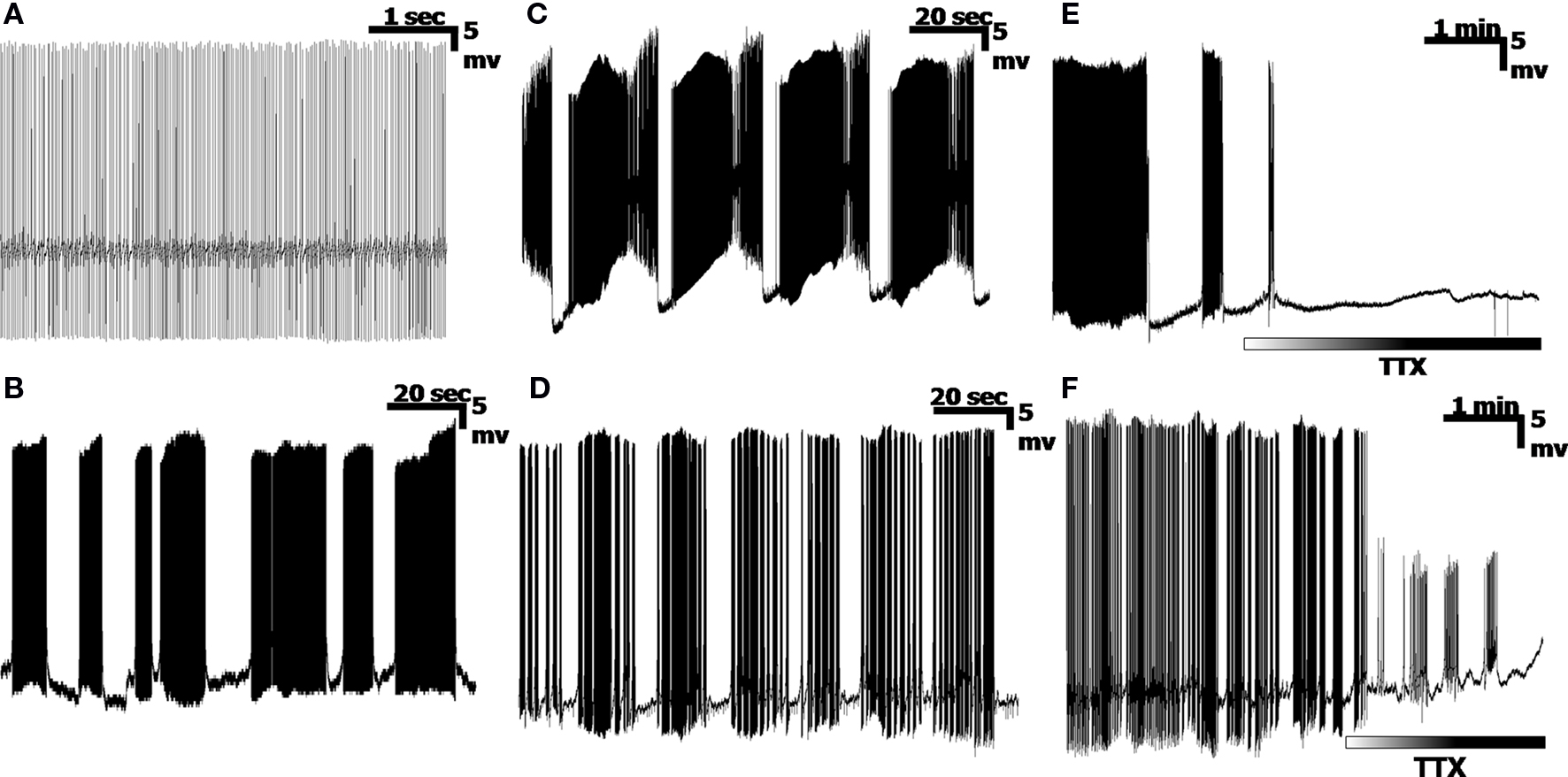
Figure 1. Examples of Purkinje cell ouput. (A) A simple spiking cell, consisting entirely of high frequency Na⁺ spikes. (B) Mostly Na⁺ spike bursts, separated by near-random pauses. (C) A trimodal state, consisting of a tonic segment of simple spikes (the upswing of each pattern), followed by a period of Ca²⁺ spike bursts (both Na⁺ and Ca²⁺ spikes), and ending in a quiescent period, in a highly cyclic pattern. (D) Bursts of Na⁺/Ca²⁺ spike bursts, separated by pauses. (E,F) Application of the Na⁺ channel blocker, TTX, removes the Na⁺ spikes, leaving either a quiescent recording (E), or bursts of Ca²⁺ spikes (F).

Definition of the Switching Frequency

The recurrence of large, periodic pauses in the PC signal is apparent in many signals. Long, recurrent pauses have been described in synaptically driven switching of the PC between states of quiescence and activity (“off” and “on” states, respectively) (Chang et al., 1993 ; Loewenstein et al., 2005 ; Rokni and Yarom, 2009 ). The frequency at which such switching occurs is hereby defined as a “Switching” frequency that can be analyzed separately from the Sodium and Calcium frequencies. When viewing a recording at large time-scales, the Switching frequency appears as a square-wave, with the “on” cycle appearing as a burst of firing (the “dark” regions in Figures 1 B–D,F). The Switching frequency’s period can be measured from the beginning/end of an “on” state to the next (or, conversely, between consecutive “off” states). Since the Switching frequency is not known to be associated with a particular ion channel, it is only seen in conjunction with the Na⁺ and Ca²⁺ spikes, and can only be defined in a firing cell. It also remains outside the general range of oscillation frequencies analyzed in the cerebellum (Maex and De Schutter, 2005 ; De Zeeuw et al., 2008 ).

Purkinje Cell Output Can be Defined by three Independent Frequencies

The interplay between the three frequencies is more than simply an additive combination, and can be described in terms of Amplitude and Frequency Modulations (AM and FM). Figure 2 A displays a generic, artificial, decomposition of a nested signal that is made up of a combined AM + FM signal, and illustrates the different underlying frequencies, with each panel being a close-up of the one above it. The overlying Switching frequency (red, top panel) represents a form of AM, where the pulses of the underlying Envelope frequency (blue) are modulated to the amplitude (i.e., on/off) of the Switching frequency, and lie within each “on” state of the square-wave. Each Envelope (blue, middle panel) frequency cycle modulates the carrier frequency (green, bottom panel), whereby the rising amplitude of the Envelope corresponds to a transient rise in the frequency of the Carrier signal (FM). The final output of the system is manifested in the form of the Carrier signal, with the information transmitted being a function of all the frequencies involved in its modulation. Figure 2 B describes a nearly identical version of this simplified frequency decomposition using a representative PC output recording containing these three frequencies. Here, the Na⁺ spikes (green, analogous to the Carrier signal) are frequency modulated to each Ca²⁺ spike (blue, analogous to the Envelope frequency), which further lie within larger AM Switching pulses (red).

FIGURE 2

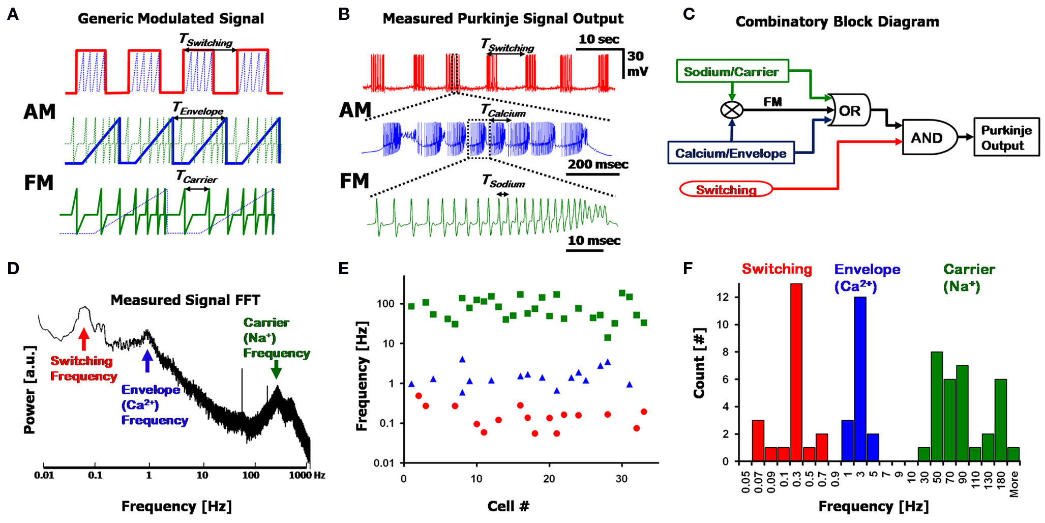
Figure 2. Frequency decomposition of the Purkinje output. (A) A generic signal displaying three nested frequencies; The Switching frequency (red) Amplitude Modulates (AM) an Envelope frequency (blue), which further Frequency Modulates (FM) the Carrier frequency (green). Each panel is a close-up of the segment above it. (B) A recording from a Purkinje cell, showing a similar modulation pattern as in (A), with the Switching, Calcium and Sodium frequencies. (C) A simplified block diagram describing the combinatory aspect of the Purkinje cell output using a logical circuit synthesis. (D) Fourier transform (power spectrum) of the signal in (B), clearly displaying the three fundamental frequencies as isolated peaks in the spectrum. (E) Location of the major peaks detected in the Fourier transforms of n = 33 cells (7 min recordings for each, with no pharmacological agents applied). The three frequency bands are split into the Switching (red, circles), Calcium (blue, triangles) and Sodium (green, squares) ranges. Note the possible overlap in the Switching and Calcium frequencies, and that the y-axis is logarithmic. (F) Histogram of the data in (E) displaying the 3 frequency bands.

The three frequencies described above can be combined in a logical circuit block diagram as illustrated in Figure 2 C. In this simplified circuit, Sodium and Calcium frequencies can function individually (“OR”) or be combined as an FM signal, and are nested within the Switching frequency (“AND”) such that the Switching frequency modulates segments of quiescence and firing. While this circuit diagram serves as a useful way for describing the three frequencies and their combinatory aspect, the experimental substantiation for the existence of these three frequencies is seen in the FFT of a PC output signal (Figure 2 D. The power spectrum is the absolute value of the Fourier transform). Long segments of signal are required to obtain a visible peak in the Switching frequency regime, which can be as long as 45 s (i.e., requiring at least 450 s of recording for an unambiguous FFT representation of the signal). The three frequencies exist in non-overlapping regions of the frequency spectrum, with the Sodium frequency typically in the order of 30–300 Hz; Calcium frequency at 1–15 Hz, and Switching frequencies at less than 1 Hz. Peaks in the spectra signify an inherent frequency in the system; however, artifacts due to higher-harmonics of the frequencies may lead to additional peaks as well.

The three frequencies appear in various combinations in PC recordings, with the sole exception that the Switching frequency does not appear by itself (six combinations in total). These combinations can be seen in the frequency spectra of different cells: Peaks in the spectra (such as Figure 2 D) reveal the existence of each frequency in the recording, and broadening of the peaks signifies a temporal drift in frequency values. By selecting peaks in the FFTs (see Materials and Methods, Section Harmonic Oscillator Statistics) of n = 33 cells, the three described frequency bands can be seen in the scatter plot of Figure 2 E, and the corresponding histogram in Figure 2 F. The Sodium frequency consists of high frequency (>30 Hz) spikes; the Calcium frequency exists in a range between 1 and 15 Hz, as has been described before (Womack and Khodakhah, 2004 ; McKay et al., 2005 ); the Switching frequency is in the sub-1 Hz region (Llinás and Sugimori, 1980 ; Chang et al., 1993 ) with spectra typically displaying more than one peak in this region as a result of artifacts due to the non-symmetrical aspect of the on/off cycles (i.e., square-wave-like waveform).

In this population of cells (n = 33, in Figures 2 E,F), the Sodium frequency band could always be seen (green) at high frequencies, in every FFT, but with a wide distribution (i.e., large FWHM, see below). The Calcium frequency (blue) was apparent in n = 16/33 cells, and a Switching frequency peak (red) was seen in n = 16/33 cells. Most of these cells had small peaks in the FFTs for the Calcium and Switching peaks (2 > Q > 0.5), signifying local variations in time (local drift) and fraction of the 7 min recording in which they occurred. There was no overall drift due to the whole-cell patch, with the results presented here quite similar to those presented by others using extracellular recording methods (see also: Womack and Khodakhah, 2002 , 2004 , reporting trimodal states for up to 2 h). The Switching and Sodium frequencies are distinct from the Calcium frequency in that their frequency bands encompass more than one order-of-magnitude. While there is no overlap between the Calcium and Sodium frequency bands, the Switching and Calcium bands overlap at ∼1 Hz, leading to ambiguity in distinguishing the two in the range of 0.5–1 Hz. In these cell recordings the frequency bands from the data were: Sodium: 85 ± 50 Hz; Calcium: 1.6 ± 0.9 Hz; Switching: 0.18 ± 0.13 Hz (±standard deviation), with respective quality factors of: Q_Na = 3.1 ± 2.2; Q_Ca = 7.2 ± 9.6; Q_Sw = 7.4 ± 6. The range for the Switching frequency is limited here by the resolution of the FFT at frequencies below 0.1 Hz. The large standard deviation for each frequency and respective quality factor signifies the wide variation between cells. In addition, the quality factor is dependent upon the amount of time the frequency existed within the 7 min recording; thus, certain segments of the recording can show extremely high Q for short times when measured independently (for example, the latter half of a trimodal state can result in Q_Ca > 40 for over a minute of recording).

Simulation of Purkinje Cell Output Using a Signal Processing Model

The three frequency AM/FM signal description is easily emulated in a computer simulation of the signal, which uses only basic signal processing tools. By combining the three frequencies, a signal similar to than shown in Figure 2 B is obtainable, as is presented in Figure 3 A. Random Gaussian noise and random temporal frequency fluctuations were added to the three fundamental frequencies to broaden the peaks in the signal’s FFT (Figure 3 B), to more realistically emulate a physiological signal. The temporal drift was low (<10%, per frequency), with the values taken from our experimental results, and which match previously reported values for these frequencies (Womack and Khodakhah, 2004 ; Achard and De Schutter, 2008 ) (frequencies displayed in the figure: 0.02, 7 and 110 Hz for the Switching, Calcium/Envelope and Sodium/Carrier frequencies, respectively). The Sodium peak in the spectrum is broadened by the frequency modulation as well, such that the Sodium frequency peak consists of the initial Sodium frequency, as well as side-lobes at the Calcium frequency (i.e. for f_Calcium = 7 Hz and f_Sodium = 100 Hz, the Sodium peak will consist of peaks at 93, 100 and 107 Hz, as in Figure 3 C, left).

FIGURE 3

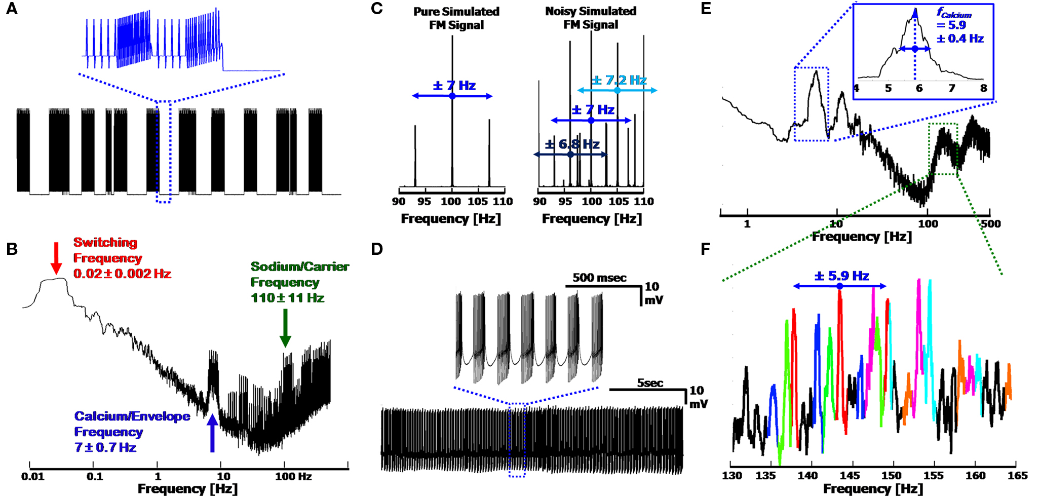
Figure 3. Simulated output signal and frequency modulation, using the three frequency model. (A) Reproduction of the signal displayed in Figure 2 B. Inset: Close up of the simplified Ca²⁺ spikes (simulated as sawtooth waveforms) with FM Na⁺ spikes, at the end of a Switching cycle. (B) FFT of the signal in (A). The three frequencies used were physiologically relevant, as described in the text. Broadening of the peaks is due to Gaussian noise and temporal fluctuations (<10%) modeled into the signal. (C) FM spectra of the Sodium signal in (A) with and without the noise added (Left and Right, respectively). Modulated Sodium frequencies include both Upper and Lower Side-Bands (USB/LSB). Noisy signals produce multiple peaks, convoluting the appearance of the side-bands, and widening the frequency bandwidth of the Sodium frequency. (D) 20 s signal from a Ca²⁺ spiking cell; Inset: Close up of Ca²⁺ bursts with FM Na⁺ spikes. (E) Spectra of signal in (D), displaying a clear Calcium frequency peak at 5.9 Hz. The Full-Width at Half Maximum provides the error of ± 0.4 Hz. (F) Close up of the Sodium frequency range in (E). Each set of peaks is color coded to display the central Carrier frequency, along with its USB and LSB, demonstrating the expected modulation frequency offsets of ∼5.9 Hz. The leftmost black peak can be seen as a second order harmonic of the red peaks, at a distance of 11.8 Hz from the central red peak. Overlapping peaks distort the amplitude of each peak, preventing quantitative analysis of the modulation.

Modulation of the Sodium Frequency by the Calcium Frequency

The modulation of the Sodium frequency to the Calcium frequency is visible in the FFT of a recorded signal, appearing as Upper and Lower Side Bands (USB/LSB), offset from the Sodium/Carrier frequency peak. In a pure FM system (Figure 3 C, Left, simulated), the USB/LSB appear in multiple harmonics away from the central peak such that the peak consists of: f_Sodium + n·f_Calcium − n·f_Calcium (with n = 1,2,3,…) (Oppenheim and Willsky, 1983 ). These harmonics typically have lower amplitudes in the frequency spectrum than the central peak at f_Sodium. The higher harmonics of the modulation (viz. all n ≥ 2) are visible as a function of the degree of modulation such that at low levels of modulation only the first set of USB/LSBs are visible. In a noisy system, or one with varying envelope and carrier frequencies, it may be difficult to distinguish between the harmonics and central peaks of the Carrier (Figure 3 C, Right). In addition, a system with combined AM and FM will result in a shift in the amplitudes of the USB and LSB in the Fourier spectrum, which would otherwise be of equal height in a pure FM system. Sampling of the signal must be above the Nyquist frequency (2·bandwidth) in order to prevent additional peak artifacts to appear in the spectrum as well.

The Frequency modulation of the Sodium frequency to the Calcium frequency can be seen in segments of recorded signal output. Figure 3 D displays a 20 s recording of a PC firing clear CaS, activated via kainate application (as described in Section Low Level Activation of the Purkinje Cell Reveals Calcium Frequencies below). When viewing the full FFT (Figure 3 E), a clear Calcium peak can be seen (here at 5.9 Hz) along with the associated harmonic artifacts, and the Sodium frequency appears as a broad band (centered at ∼150 Hz). The width of the Calcium peak displays the variation of the frequency over time (FWHM of 0.4 Hz, which is related to the standard deviation). The modulation of the Sodium frequency is apparent only when closely examining the Sodium frequency band in detail. Figure 3 F displays the Sodium frequencies color coded to emphasize the probable USB/LSB of each peak. Overlap, or superposition, of the peaks causes the distortion of the true amplitudes of each peak. Due to the varying nature of the Sodium and Calcium frequencies, it is non-trivial to ascertain the degree of modulation in the system, with only first order USB/LSBs being distinctly visible as near-constant offset side bands (of 5.9 Hz). Higher harmonics of the FM signal consist of additional peaks in the spectrum, further complicating the distinguishing of the individual peaks. The small degree of additional AM of the Sodium frequency (apparent in the small upswing of the Na⁺ spikes in the inset of Figure 3 D) adds asymmetry to the USB/LSB as well. This is demonstrated in the red set of peaks in Figure 3 F (centered at 143.7 Hz), which display both an asymmetry of the USB/LSB, and a possible 2nd order peak on the left-hand side of the spectrum (at 143.7–2·5.9 ≈ 132 Hz, in black).

Analysis of Calcium Frequency Via Pharmacological Activation

The Calcium frequency range described in Section “Purkinje Cell Output can be Defined by Three Independent Frequencies” for non-pharmacologically affected PCs (1.6 ± 0.9 Hz, see also De Zeeuw et al., 2008 ) is lower than that described for CaS in other reports (Womack and Khodakhah, 2002 ; McKay et al., 2005 ). Attributing the CaS to the delta or theta oscillation bands, known from other regions of the brain (Buzsáki and Draguhn, 2004 ; De Zeeuw et al., 2008 ), is therefore ambiguous. To address this issue, we selectively activated the CaS in PCs in vitro using various pharmacological agents, and analyzed the inherent CaS firing capabilities of the PCs.

Low Level Activation of the Purkinje Cell Reveals Calcium Frequencies

Since the threshold of the Ca²⁺ spikes is a few mV higher than the Na⁺ spikes (5–15 mV), a low level depolarization of the PC will artificially induce the activation of the Calcium frequency, in addition to the lower-threshold Sodium frequency (Häusser and Roth, 1997 ). Therefore, a low level activation of the PC can be used to investigate the behavior of the Calcium frequency. In PCs, excitatory ionotropic synaptic transmission occurs primarily via the AMPA receptors, with kainate receptors being the minority (≤5%) of ionotropic Glutamate Receptors (iGluRs) ( Häusser and Roth, 1997 ; Huang et al., 2004 ). The current induced by kainate receptor activation is ∼5% of the overall current typically obtained upon full glutamatergic activation, and therefore, by selectively stimulating only the kainate receptors, one can activate the CaS without overwhelming the cell. Moreover, it is known that Calcium permeates kainate receptors (Brorson et al., 1992 ). The activation of kainate receptors is possible either through a selective kainate receptor agonist (ATPA, 1–15 µM), or a combination of glutamate and AMPA antagonist (MSG and GYKI at 100, 10 µM, respectively). Low dosages of AMPA agonist (5-FWD, 0.1 µM, n = 6 cells) or MSG (100 µM) alone induces a fast acting depolarization block that renders the cell incapable of firing, with the membrane potential pegged at ≈−45−40 mV, and is therefore not useful for measuring the CaS over time.

Application of the kainate receptor agonist ATPA (1–15 µM) induces the firing of CaS in all cells measured (100% activation of CaS in n = 38/38 cells), regardless of the firing pattern exhibited before the application of the agonist (as illustrated in the transition between Figures 4 A,B). The Sodium frequency could be removed by the additional (or prior) application of TTX (1 µM), in which case only the underlying CaS remain (Figure 4 C). The addition of ATPA to a cell causes it to fire CaS for 1–3 min before undergoing a depolarization block (at ∼−40 mV), at which point the cell no longer fires. This depolarization block could be removed by adding the ionotropic glutamate receptor blocker, DNQX (10 µM), which reverts to a combined SS/CaS firing mode (Figure 4 D), suggesting that the cell was not irreversibly affected by the induction of CaS, and could still fire in the frequency ranges seen prior to the kainate receptor activation. Application of the GABA_A and GABA_C receptor blockers, GABAzine (10 µM) and picrotoxin (PTX, 100 µM), and the glycine receptor blocker, strychnine (1 µM), did not significantly affect ATPA induced CaS (n = 15 cells, p > 0.5 two sample, unequal variance t-test), suggesting that this effect is not mediated by inhibitory interneurons.

FIGURE 4

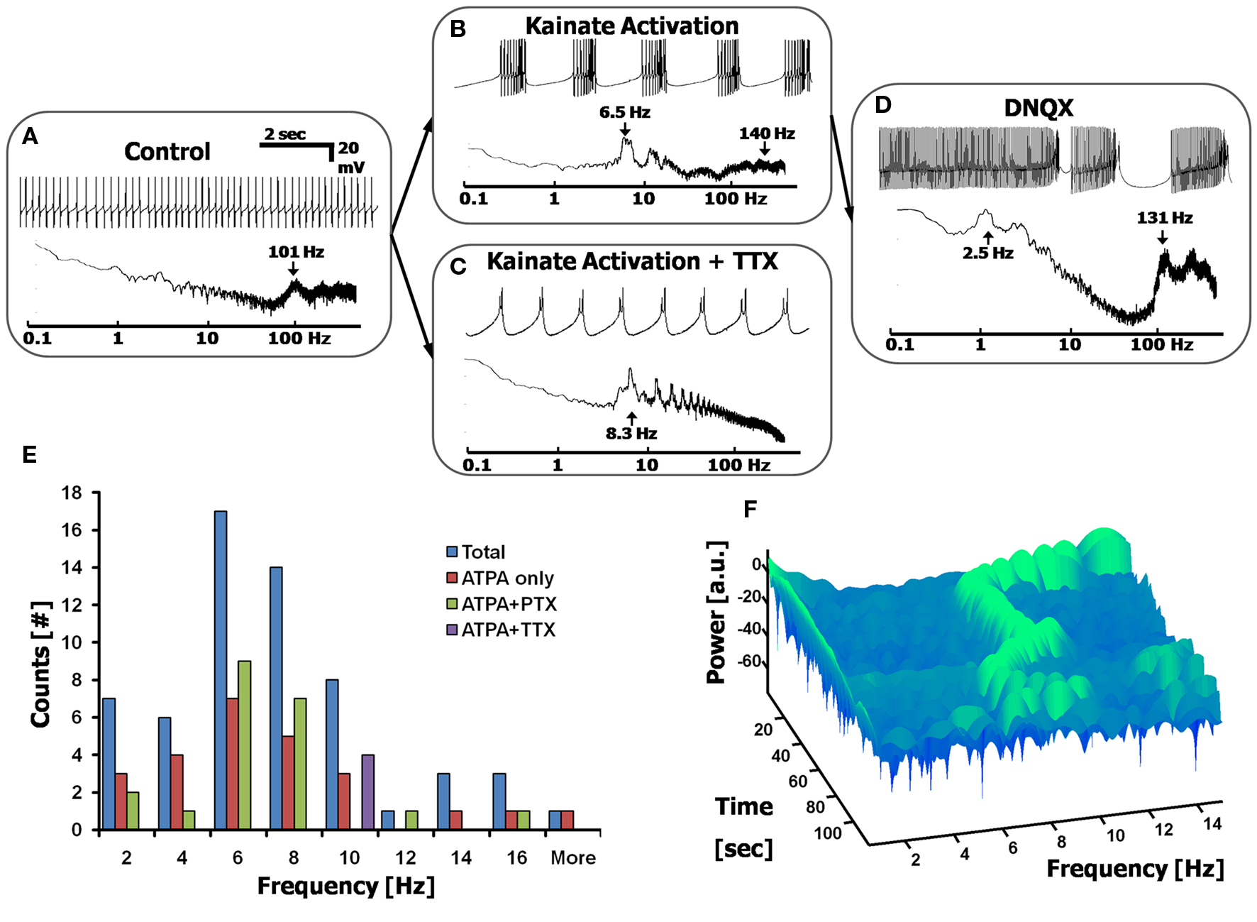
Figure 4. Calcium frequency analysis via low-level depolarization using kainate receptor agonists. (A) Control cell displaying simple spikes only. Top: current-clamped recording; Bottom: Fourier spectrum. (B,C) Adding a kainate receptor agonist, ATPA (15 µM) induces Ca²⁺ spikes in all cells, showing Ca²⁺ spike bursts in most cells (B), or only Ca²⁺ spikes in cells pretreated with 1 µM TTX (C). (D) The blocker DNQX (10 µM) reverts cells back to a state of combined Na⁺ and Ca²⁺ spikes (n = 14/21 cells). (E) Histogram displaying the range of Ca²⁺ spikes induced via low-level depolarization of kainate receptors, giving a frequency distribution centered at ∼6 Hz (n = 38 cells). Both ATPA and ATPA + PTX give the same distribution, thereby excluding the effects of inhibitory interneurons. ATPA + TTX appear to shift the Calcium frequency to the right. (F) A 3D spectrogram displaying the dynamic changes in the Calcium frequency over time, after the application of ATPA. Each row (in time) represents a 3 s FFT, centered on the Calcium frequency. Green signifies a local peak in the Calcium frequency spectrum, as a function of time.

The Calcium Frequency is Centered at 6 Hz and Show Time-Dependent Transitions

The distribution of frequencies of CaS was reliably obtained by stimulating kainate receptors using a variety of drug combinations (See Materials and methods). We report that this distribution of frequencies is centered at 6 Hz (6.3 ± 3.5 Hz, Figure 3 E, n > 30 cells, with data points taken from the FFTs). The Calcium frequency appears to be cell dependent, and lies near a similar band to the theta frequency (4–10 Hz) seen in other cortical systems (Buzsáki and Draguhn, 2004 ; De Zeeuw et al., 2008 ). The distribution of frequencies is not affected by the co-application of inhibitory receptor blockers (such as PTX). However, there does appear to be a rightward shift of frequencies when applying TTX (n = 4 cells, p < 0.031 two-tailed KS test), as has been previously reported (Womack and Khodakhah, 2004 ).

The precise frequency of the CaS is not constant, and changes over time, within the Calcium frequency band range. This can be seen when using a Short-Time Fourier Transform (STFT) analysis of the Calcium frequency region, beginning at the time the ATPA took effect, displayed in a representative spectrogram in Figure 4 F. The spectrogram displays the peaks in the FFT as a function of time for a given frequency range, and shows variations in peak frequency over time. Each row (in time) of the spectrogram represents a segment of the FFT within the time slot, with the width of each row required to be at least ∼10 cycles of the period under analysis (i.e, for a 7 Hz signal, each time window must be at least 10·1/7 s ≈ 1.4 s). Discontinuities and shifts in the frequency over time were seen in all cells measured with the Calcium frequency activation experiments.

Frequency Doubling and Steady-State Decay of the Calcium Frequency

The shifts in the Calcium frequency over time seen in the spectrograms display two distinct phenomena: discontinuities in the spiking frequency, and the gradual decay to a steady-state (constant) spiking frequency value.

Figures 5 A,B present spectrograms displaying abrupt discontinuities in the frequency. In cells showing these discontinuities, the frequency usually jumped to a frequency exactly double the initial frequency (n = 8/19 cells, with ATPA). This frequency doubling is not an artifact of the STFT technique, which can also display multiple harmonics of a signal, but is seen in the time domain as well. This is demonstrated in Figure 5 C, which displays the doubling of the Calcium frequency as a splitting of the CaS (which include AM Na⁺ spikes) into two, within a short (<2 s) transition time, during which both frequencies exist in the cell.

FIGURE 5

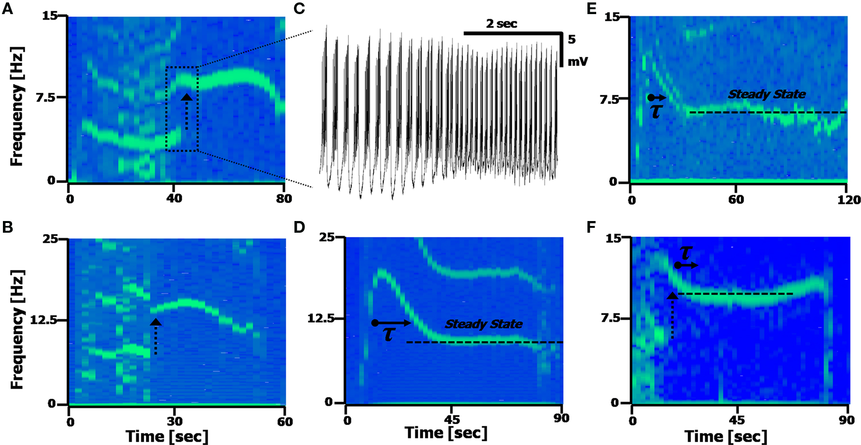
Figure 5. Calcium frequency transitions. (A,B) Spectrograms displaying discontinuities in the frequency, with a frequency doubling of the Ca²⁺ spikes. Arrow represents the frequency doubling. (A) Shift from 4.5 to 9 Hz; (B), shift from 7 to 14 Hz. (C) Time-domain recording of the transition point between the two frequencies occurring in (A). (D,E) Spectrograms displaying a transient decay to a steady state frequency. (C) τ = 7.2 s; (D) τ = 8.1 s. The second harmonic artifact of the Ca²⁺ spikes is distinctly visible in (A,B and D). (F) A spectrogram displaying both a frequency doubling, followed by a steady-state recovery transient.

Figures 5 D,E present spectrograms displaying a decay from an initial spiking frequency to a steady-state. This frequency transition involves a single-exponential decay from a higher Calcium frequency to a lower one, and remaining at that constant level. In these cells (n = 9/19, with ATPA), the average time constant was found to be τ = 8.2 ± 2.6 s, with an average change in frequency of Δf = 4.6 ± 2.8 Hz, as measured assuming an exponential decay [i.e. assuming a function proportional to: f_Ca – Δf·exp(–t/τ)]. Some cells (n = 6/19) exhibited both the frequency doubling and an exponential decay phenomena simultaneously (Figure 5 F).

The dynamic transitions described here show the deviations the Calcium frequency can have away from its central range (f_Ca centered around 6 Hz, from Figure 4 E), with some cells displaying more than one fundamental frequency occurring in the same time window (n = 4/19 cells). These phenomena are some of the reasons the Calcium frequency peak in the FFT will appear broader and asymmetric, with the asymmetry caused by the tail of the exponential decay broadening the frequency peaks.

The Switching Frequency and Pauses in Purkinje Cell Recordings

The cyclical patterns seen in PC recordings leads to the defining of the Switching frequency as an inherent, fundamental frequency of the PC. This frequency has not been well characterized in the past (Chang et al., 1993 ; Maex and De Schutter, 2005 ; De Zeeuw et al., 2008 ), and signifies the possibility of a pace-making function of the PC in cerebellar circuitry (Jacobson et al., 2008 ; Rokni et al., 2009 ). The Switching frequency would adequately describe the existence of cyclical bimodal and trimodal states, as well as other repetitive pausing seen in PCs (as in Figure 1 ), since the repetition of pausing would merely be the “off” state of a Switching cycle. This assumes a cyclical pattern to the Switching frequency, which we have shown to be the case in many cells in vitro. The ability of synaptic inputs to modulate these pauses ( Loewenstein et al., 2005 ; Hong and De Schutter, 2008 ) adds a possible asynchronous method of changing the modulatory pattern of the Switching frequency, adding to the apparent “randomness” of measured PC signals in vivo (Keating and Thach, 1997 ; Kitazawa and Wolpert, 2005 ; Schonewille et al., 2005 ; Hakimian et al., 2008 ). Describing the pauses in the PC signal as stochastic in origin would elucidate both the broadening of the peaks in the FFTs of the Switching frequencies, and would explain why it is not always seen: only 16 of the 33 cells in Figure 1 E had a measureable peak. However, of these 16, 84% had a quality factor (Q ≡f_peak/FWHM) of over 2 (n = 14/16 cells) and 25% (n = 4/16 cells) had a Q of over 5. In the harmonic oscillator description of the PC, having a high Q (Q > 1/2) signify the ability to oscillate without dissipation.

Photo-Switching the Calcium and Switching Frequencies

Using a newly developed, highly specific, reversibly photo-switching kainate receptor agonist (see Materials and methods, Volgraf et al., 2007 ), we were able to modulate the Calcium and Switching frequencies by modulating the light input onto the cell (n = 3 cells with 50 µM of agonist alone; n = 9 with 100 µM agonist, 1 µM TTX and 10 µM GYKI). As described above, there is a link between activating the kainate receptors on a PC (using pharmacological agents such as ATPA) and the Calcium frequency. This is possibly due to the permeability of Ca²⁺ via kainate receptors (Brorson et al., 1992 ), and the large number of kainate receptors on a PC (Wisden and Seeburg, 1993 ). Using this photo-switchable agonist, the Calcium and Switching frequencies were externally modulated.

Using the photo-switchable agonist alone (n = 3) and switching the wavelength of light illuminating the cell through the microscope from cyan (500 nm) to UV (380 nm), the PC exhibits a change in frequency of the CaS (Figures 6 A,B). In 10-s illumination of UV, the Calcium frequency is increased, resulting in more CaS (Figure 6 B, right), followed by a decrease in 10 s of cyan light. For the cell recording displayed in Figure 6 B, the cell was firing CaS before the photo-switching (in the presence of 50 µM of the photo-switchable agonist) at a rate of 1.18 ± 0.23 Hz, and during the UV illumination period, at a rate of 1.88 ± 0.37 Hz (p < 0.01, two tailed t-test). Comparing the cyan and UV showed a distinct difference, with a 2 Hz change in CaS frequency between the two regions (p < 0.01, two-tailed t-test, ignoring the overlap between windows), displaying the range of modulation of the Calcium frequency in this cell.

FIGURE 6

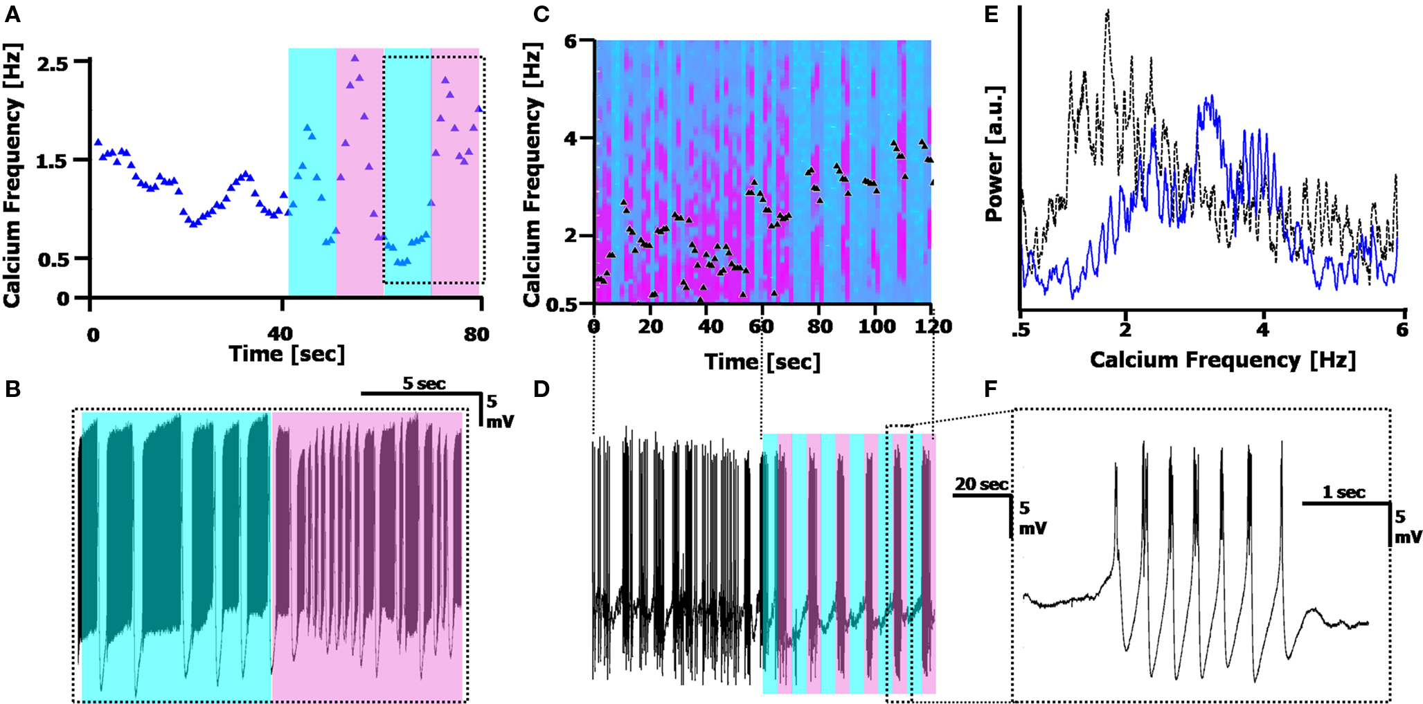
Figure 6. Reversible photo-switching of the calcium frequency. (A) Frequency tracking the Calcium frequency range of a cell in 50 µM of the reversibly photo-switchable kainate receptor agonist, with 10 s cyan, 10 s UV illumination (500 and 380 nm, respectively; shaded region). The Calcium frequency rises under UV illumination, and generally decreases in cyan illumination. (B) Recording of the cell during the 10/10 illumination pattern is delineated in the dotted box in (A), displaying the frequency change. (C) Spectrogram of the Calcium frequency before (0–60 s) and during (60–120 s) illumination with 5 s cyan/5 s UV, in the presence of 100 µM photo-switchable agonist, 1 µM TTX and 10 µM GYKI. Black triangles mark the peak position of the Calcium frequency. (D) Recording of the cell, displaying the illumination pattern. The time scale matches that of (C). (E) Fourier spectrum of the Calcium frequency before (dotted black line) and during (solid blue line) illumination, displaying the rightward shift in Ca²⁺ spikes during (UV) illumination. This spectrum does not provide information on the Switching frequency (out of range). (F) A single burst of Ca²⁺ spikes during one of the UV illumination cycles in (D).

Using the photo-switchable agonist while simultaneously blocking Na⁺ channels with TTX (1 µM) and AMPA receptors via GYKI (10 µM) blocked the Sodium frequency completely, and resulted in the CaS completely following the photo-induced modulation (Figure 6 C,D, n = 9). As demonstrated in Figures 6 C–F, before illuminating the cell with 5 s cyan/5 s UV, the cell fires CaS at a wide range of frequencies between 1–3 Hz (Figure 6 E, dotted black line). During cyan illumination, there is a cessation of firing, and during UV illumination, the cell fires CaS at a higher frequency (3.36 ± 0.33 Hz during UV as opposed to 1.5 ± 0.62 Hz before illumination). The spectrogram in Figure 6 C plots the shifts in frequency over time, along with the peak frequency (black triangles). A FFT of the region before and during illumination (Figure 6 E, 60 s each) displays the shift in Calcium frequency, however it does not clearly display the additional photo-modulation. The external Switching modulation applied here was 10 s (5 s cyan = off/5 s UV = on), and the cells always followed the external modulation almost perfectly (in the cell in Figures 6 C–F, the Switching frequency during the illumination period is 10.6 ± 1.36 s).

Modulation of the Calcium frequency is possible since the compound is reversible, allowing us to inspect the effects of kainate receptor activation in a way that pharmacological application of traditional kainate agonists cannot. For any cell, we were able to alternate between rapid firing in UV and slower/no firing in cyan by switching the illumination wavelength. The cells would revert to the slower Calcium frequency after the light was turned off, with the Calcium frequency always being less in the dark than the UV, and more than the Cyan (p < 0.01 for both, as described above).

Discussion

Our work here describes the Purkinje cell in terms of its fundamental frequencies. This approach is based on signal processing analysis, assuming an oscillatory behavior of the PC output. Using tools such as FFTs, we are able to distinguish three intrinsic frequencies in the PC output – the Sodium, Calcium and Switching frequencies, show some of the modulatory effects of these frequencies upon one another, and demonstrate modulation of the frequencies upon external input. These frequencies are quite apparent in in vitro preparations, and point to the natural harmonic oscillator capabilities of the PC irrespective of its synaptic inputs, which may make the detection of such frequencies difficult in synaptically active in vivo preparations (Keating and Thach, 1997 ).

The important aspect of the FFT studies is in the frequency range involved: Typical studies of the cerebellum have focused on frequency ranges that have been similar to those seen in cortical networks (Keating and Thach, 1997 ; Maex and De Schutter, 2005 ; De Zeeuw et al., 2008 ), and for the most part, the sub-Hz range has been ignored in nearly all studies of the PC, which requires long segments of recording to analyze. However, even in studies with long recordings (Keating and Thach, 1997 ; Womack and Khodakhah, 2002 , 2004 ; McKay et al., 2007 ; Hakimian et al., 2008 ) the range of frequencies studied has typically been focused upon higher frequencies, typically in order to associate the rhythms seen in the cerebellum with those in the cortex (De Zeeuw et al., 2008 ).

Calcium Frequency

The Calcium frequency is here described as being in the range of ∼1–15 Hz, with lower frequencies seen in control studies with no pharmacological agents and higher ones in the presence of a kainate receptor agonist. This range of CaS has been previously been reported in in vitro preparations (Womack and Khodakhah, 2004 ; McKay et al., 2005 ; Achard and De Schutter, 2008 ), however this is the first time it has been shown how easily the CaS can be activated by kainate receptors (100% activation of CaS). Our studies show that this frequency is time dependent, with double-frequency shifting and the steady-state decay in the ATPA studies, and up-shifting of frequency in the photo-switchable agonist studies. The frequency doubling described here appears to be the first of its kind in any neuronal system, and its significance is therefore unknown. This doubling occurred only in the continual presence of ATPA, suggesting that it may not be seen in in vivo recordings, where such high dosages of kainate activation may not occur, but has yet to be studied.

The varying of the kainate activation on the cell, as demonstrated in the reversibly photo-switchable compound, can explain the variation in frequencies between the control studies (Figures 2 E,F) and the ATPA studies (Figure 4 E). It can be inferred from these experiments that the influx of Ca²⁺ through the kainate receptors (Brorson et al., 1992 ; Huang et al., 2004 ), causes a direct increase in the Calcium frequency, as demonstrated in the increase in CaS during the UV illumination in Figure 6 . The effect of modulating the Calcium frequency is also shown to have a direct effect on the Sodium and Switching frequency, via AM and FM processes, resulting in an analog modulation of the final series of action potentials emanating from the PC. Similar forms of AM have recently been shown in other systems (Atallah and Scanziani, 2009 ; Hartwich et al., 2009 ; Mathy et al., 2009 ), as well as recently in the PC itself (Kramer et al., 2008 ).

Switching Frequency and Bistability

One of the principal controversies in the study of the cerebellum and the PC is in the existence of bistability of the PC (Rokni et al., 2009 ). The bistability of the PC has been reported as both a recurring phenomenon in a small subset of cells (Llinás and Sugimori, 1980 ; Chang et al., 1993 ; Womack and Khodakhah, 2004 ) and also as a function of the climbing fiber input onto the cell (Loewenstein et al., 2005 ; McKay et al., 2007 ; Davie et al., 2008 ). However, it was also shown that the bistability is perhaps a byproduct of the anesthetic used in in vivo preparations (Schonewille et al., 2005 ). Despite this discrepancy, one of the predominant claims in cerebellar functional theory is that the PC acts within a closed loop circuit with the olivary nuclei (inferior olive) acting as a temporal signal generator, and the climbing fiber acting as a controller signal (Lang et al., 1999 ; Davie et al., 2008 ; Jacobson et al., 2008 ; Hong and De Schutter, 2008 ; Mathy et al., 2009 ). A parallel interpretation of PC encoding of information focuses primarily on the pauses in the firing rate (Jaeger and Bower, 1994 ; Shin et al., 2007 ; Steuber et al., 2007 ). These pauses, seen in in vivo recordings as well, are typically not considered to be oscillatory in nature.

The results presented here regarding the internal capability of the PC to fire oscillatory patterns of three fundamental frequencies is in contrast to the stochastic firing assumptions made by some of these interpretations. Since most of the experimental FFTs displayed in Figure 2 E display a high quality factor (Q > 1/2), assigning a resonance frequency to each cell is non-negligible. Pauses in the PC code can therefore be described as a function of the modulation of the Calcium and Switching frequencies, and not merely stochastic variations of the Sodium frequency. Apparent randomness in the pauses can be due to the climbing fiber input to the PC, which can act as an asynchronous reset input for the Switching frequency. This interpretation fits well with recent results that directly correlate the climbing fiber input, bistability and Ca²⁺ input to the cell (Rokni and Yarom, 2009 ), as well as our results here that show that modulation of the kainate receptors modulates the PC’s frequencies. The correlation between climbing fiber input and the activation of kainate receptors in the PC can perhaps be attributed to the surplus of the neurotransmitter release of glutamate from the climbing fiber, activating both AMPA and kainate receptors (Huang et al., 2004 ). This surplus of glutamate will then induce a complex spike, which is defined as a high frequency Ca²⁺ spike enveloping Na⁺ spikes, using the terminology described in this paper. It can therefore be the (asynchronous) synaptic modulation of the Switching and Calcium frequencies that imparts the apparent randomness of pausing in the PC output. It should also be noted that the long time scales of kainate activation here match those used in long-term depression activation in the PC-climbing fiber synapse (30 s) and the frequency of LTD stimulation protocols (5 Hz) matches those of the Calcium frequency (Hansel and Linden, 2000 ; Ito, 2001 ).

An additional question regarding the Switching frequency is the biological relevance of its slow cycle period. Slow frequencies are known to exist in other regions of the brain (Sanchez-Vives and McCormick, 2000 ; Buzsáki and Draguhn, 2004 ), but have no corollary in the cerebellum. Long bursting cycles are known to exist in many different types of neurons with similar time scales, and are an intrinsic property of the Hodgkin-Huxley equations (Izhikevich, 2006 ). Furthermore, recent in vivo studies of awake, moving rats have shown that the Bergmann glial cells, which are involved in re-uptake of spillover glutamate (Bellamy, 2006 ), have slow Ca²⁺-driven bursts in the mHz regime (Nimmerjahn et al., 2009 ), comparable to the Switching frequency seen in the PC here.

The results described here have implications towards the deciphering of the information flow from the PC in the cerebellar network. Information theory posits that any correlation existing in a system reduces the information flow (Johnson, 1980 ). Therefore, the combination of three intrinsic frequencies and their modulation using AM and/or FM limits the total amount of information the PC can transmit in terms of individual spikes, if assuming a uniform distribution of action potentials (Strong et al., 1998 ; Brunel et al., 2004 ). Instead, the variation of these frequencies over time (Shin et al., 2007 ) and bursts of firing (Lisman, 1997 ) can provide additional information.

In conclusion, this description of the PC can be described as a re-assessment of the PC output in a different space: the frequency domain. As demonstrated in this paper, viewing the PC in terms of its frequencies sheds light on new phenomena (such as frequency doubling), while also attempting to describe the vast complexity of the PC output as being a dynamically modulatable generator of harmonic signals.

Conflict of Interest Statement

The authors declare that the research was conducted in the absence of any commercial or financial relationships that can be construed as a potential conflict of interest.

Acknowledgments

Thanks to Professors Harold Lecar and Jose Carmena for their helpful discussion. Ze’ev R. Abrams would like to thank the NDSEG Fellowship for funding. This work was funded by an NSF grant.

References

Achard, P., and De Schutter, E. (2008). Calcium, synaptic plasticity and intrinsic homeostasis in Purkinje neuron models. Front. Comput. Neurosci. 8, 1–10.

Albus, J. S. (1971). A theory of cerebellar function. Math. Biosci. 10, 25–61.

CrossRef Full Text

Atallah, B., and Scanziani, M. (2009). Instantaneous modulation of gamma oscillation frequency by balancing excitation with inhibition. Neuron 62, 566–577.

Pubmed Abstract | Pubmed Full Text | CrossRef Full Text

Bellamy, T. C. (2006). Interactions between Purkinje neurones and Bergmann glia. Cerebellum 5, 116–126.

Pubmed Abstract | Pubmed Full Text | CrossRef Full Text

Bialek, W., Rieke, F., De Ruyter, R. R., and Warland, D. (1991). Reading a neural code. Science 252:1854–1857.

Pubmed Abstract | Pubmed Full Text

Brorson, J. R., Bleakman, D., Chard, P. S., and Miller, R. J. (1992). Calcium directly permeates Kainate/α(-amino-3-hydroxy-5-methyl-4-isoxazolepropionic acid receptors in cultured cerebellar Purkinje neurons. Mol. Pharmacol. 41, 603–608.

Pubmed Abstract | Pubmed Full Text

Brunel, N., Hakim, V., Isope, P., Nadal, J. P., and Barbour, B. (2004). Optimal information storage and the distribution of synaptic weights: perceptron versus Purkinje cell. Neuron 43, 745–757.

Pubmed Abstract | Pubmed Full Text

Buzsáki, G., and Draguhn, A. (2004). Neuronal oscillations in cortical networks. Science 304, 1926–1929.

Pubmed Abstract | Pubmed Full Text | CrossRef Full Text

Chang, W., Strahlendorf, J. C., and Strahlendorf, H. K. (1993). ionic contributions to the oscillatory firing activity of rat Purkinje cells in vitro. Brain Res. 614, 335–341.

Pubmed Abstract | Pubmed Full Text | CrossRef Full Text

Cheron, G., Servais, L., and Dan, B. (2008). Cerebellar network plasticity: from genes to fast oscillation. Neuroscience 153, 1–19.

Pubmed Abstract | Pubmed Full Text | CrossRef Full Text

Davie, J. T., Clark, B. A., and Häusser, M. (2008). The origin of the complex spike in cerebellar purkinje cells. J. Neurosci. 28, 7599–7609.

Pubmed Abstract | Pubmed Full Text | CrossRef Full Text

De Schutter, E., and Bower, J. M. (1994). An active membrane model of the cerebellar purkinje cell I. Simulation of current clamps in slice. J. Neurophysiol. 71, 375–400.

Pubmed Abstract | Pubmed Full Text

De Zeeuw, C. I., Hoebeek, F. E., and Schonewille, M. (2008). Causes and consequences of oscillations in the cerebellar cortex. Neuron 58, 655–658.

Pubmed Abstract | Pubmed Full Text | CrossRef Full Text

Doya, K., Kimura, H., and Kawato, M. (2001). Neural mechanisms of learning and control. IEEE Control Syst. Mag. 8, 42–54.

CrossRef Full Text

Ekerot, C. F., and Kano, M. (1985). Long-term depression of parallel fibre synapses following stimulation of climbing fibres. Brain Res. 342, 357–360.

Pubmed Abstract | Pubmed Full Text | CrossRef Full Text

Hakimian, S., Norris, S. A., Greger, B., Keating, J. G., Anderson, C. H., and Thach, W. T. (2008). Time and frequency characteristics of purkinje cell complex spikes in the awake monkey performing a nonperiodic task. J. Neurophysiol. 100, 1032–1040.

Pubmed Abstract | Pubmed Full Text | CrossRef Full Text

Hansel, C., and Linden, D. J. (2000). Long-term depression of the cerebellar climbing fiber-purkinje neuron synapse. Neuron 26, 473–482.

Pubmed Abstract | Pubmed Full Text | CrossRef Full Text

Hartwich, K., Pollack, T., and Klausberger, T. (2009). Distinct firing patterns of identified basket and dendrite- targeting interneurons in the prefrontal cortex during hippocampal theta and local spindle oscillations. J. Neurosi. 29, 9563–9574.

CrossRef Full Text

Häusser, M., and Roth, A. (1997). Dendritic and somatic glutamate receptor channels in rat cerebellar Purkinje cells. J. Physiol. (Lond.) 501, 77–95.

Pubmed Abstract | Pubmed Full Text | CrossRef Full Text

Hong, S., and De Schutter, E. (2008). Purkinje neurons: what is the signal for complex spikes? Curr. Biol. 18, 969–971.

Pubmed Abstract | Pubmed Full Text | CrossRef Full Text

Huang, Y. H., Dykes-Hoberg, M., Tanaka, K., Rothstein, J. D., and Bergles, D. E. (2004). Climbing fiber activation of EAAT4 transporters and kainate receptors in cerebellar Purkinje cells. J. Neurosci. 24, 103–111.

Pubmed Abstract | Pubmed Full Text | CrossRef Full Text

Ito, M. (2001). Cerebellar long-term depression: characterization, signal transduction, and functional roles. Physiol. Rev. 81, 1143–1195.

Pubmed Abstract | Pubmed Full Text

Ito, M. (2006). Cerebellar circuitry as a neuronal machine. Prog. Neurobiol. 78, 272–303.

Pubmed Abstract | Pubmed Full Text | CrossRef Full Text

Izhikevich, E. M. (2006). Dynamical Systems in Neuroscience: The Geometry of Excitability and Bursting. Cambridge: MIT Press.

Jacobson, G. A., Rokni, D., and Yarom, Y. (2008). A model of the olivo-cerebellar system as a temporal pattern generator. Trends Neurosci. 31, 617–625.

Pubmed Abstract | Pubmed Full Text | CrossRef Full Text

Jaeger, D., and Bower, J. M. (1994). Prolonged responses in rat cerebellar Purkinje cells following activation of the granule cell layer: and intracellular in vitro and in vivo investigation. Exp. Brain Res. 100, 200–214.

Pubmed Abstract | Pubmed Full Text | CrossRef Full Text

Johnson, K. O. (1980). Sensory discrimination: neural processes preceding discrimination decision. J. Neurophysiol. 43, 1793–1815.

Pubmed Abstract | Pubmed Full Text

Kano, M., and Kato, M. (1987). Quisqualate receptors are specifically involves in cerebellar synaptic plasticity. Nature 325, 276–279.

Pubmed Abstract | Pubmed Full Text | CrossRef Full Text

Keating, J. G., and Thach, W. T. (1997). No clock signal in the discharge of neurons in the deep cerebellar nuclei. J. Neurophysiol. 77, 2232–2234.

Pubmed Abstract | Pubmed Full Text

Kitazawa, S., and Wolpert, D. M. (2005). Rythmicity, randomness and synchrony in climbing fiber signals. Trends Neurosci. 28, 611–619.

Pubmed Abstract | Pubmed Full Text | CrossRef Full Text

Kramer, M. A., Traub, R. D., and Kopell, N. J. (2008). New dynamics in cerebellar purkinje cells: torus canards. Phys. Rev. Lett. 101, 068103–068106.

Pubmed Abstract | Pubmed Full Text | CrossRef Full Text

Lang, E. J., Sugihara, I., Welsh, J. P., and Llinás, R. (1999). Patterns of spontaneous purkinje cell complex spike activity in awake rat. J. Neurosci. 18, 2728–2738.

Lisman, J. E. (1997). Bursts as a unit of neural information: making unreliable synapses reliable. Trends Neurosci. 20, 38–43.

Pubmed Abstract | Pubmed Full Text | CrossRef Full Text

Llinás, R., and Sugimori, M. (1980). Electrophysiological properties of in vitro Purkinje cell dendrites in mammalian cerebellar slices. J. Physiol. (Lond.) 305, 197–213.

Pubmed Abstract | Pubmed Full Text

Loewenstein, Y., Mahon, S., Chadderton, P., Kitamura, K., Sompolinsky, H., Yarom, Y., and Häusser, M. (2005). Bistability of cerebellar Purkinje cells modulated by sensory stimulation. Nat. Neurosci. 8, 202–211.

Pubmed Abstract | Pubmed Full Text | CrossRef Full Text

Maex, R., and De Schutter, E. (2005). Oscillations in the cerebellar cortex: a prediction of their frequency bands. Prog. Brain Res. 148, 181–188.

Pubmed Abstract | Pubmed Full Text | CrossRef Full Text

Marr, D. (1969). A theory of cerebellar cortex. J. Physiol. (Lond.) 202, 437–470.

Pubmed Abstract | Pubmed Full Text

Mathy, A., Ho, S. S. N., Davie, J. T., Duguid, I. C., Clark, B. A., and Häusser, M. (2009). Encoding of oscillations by axonal bursts in inferior olive neurons. Neuron 62, 388–399.

Pubmed Abstract | Pubmed Full Text | CrossRef Full Text

McKay, B. E., Engbers, J. D. T., Mehaffey, W. H., Gordon, G. R. J., Molineux, M. L., Bains, J. S., and Turner, R. W. (2007). Climbing fiber discharge regulates cerebellar functions by controlling the intrinsic characteristics of purkinje cell output. J. Neurophysiol. 97, 2590–2604.

Pubmed Abstract | Pubmed Full Text | CrossRef Full Text

McKay, B. E., Molineux, M. L., Mehaffey, W. H., and Turner, R. W. (2005). Kv1 K⁺ channels control purkinje cell output to facilitate postsynaptic rebound discharge in deep cerebellar neurons. J. Neurosci. 25, 1481–1492.

Pubmed Abstract | Pubmed Full Text | CrossRef Full Text

Nimmerjahn, A., Mukamel, E. A., and Schnitzer, M. J. (2009). Motor behavior activates bergmann glial networks. Neuron 62, 400–412.

Pubmed Abstract | Pubmed Full Text | CrossRef Full Text

Oppenheim, A., and Willsky, A. S. (1983). Signals and systems. Englewood Cliffs, NJ: Prentice Hall Inc.

Pedregal, C., Collado, I., Excribano, A., Ezquerra, J., Domnguez, C., Mateo, A. I., Rubio, A., Baker, S. R., Goldsworthy, J., Kamboj, R. K., Ballyk, B. A., Hoo, K., and Bleakman, D. (2000). 4-alkyl- and 4-cinnamylglutamic acid analogues are potent glur5 kainate receptor agonists. J. Med. Chem. 43, 1958–1968.

Pubmed Abstract | Pubmed Full Text | CrossRef Full Text

Roberts, W. M. (1979). Optimal recognition of neuronal waveforms. Biol. Cybern. 35, 73–80.

Pubmed Abstract | Pubmed Full Text | CrossRef Full Text

Rokni, D., Tal, Z., Byk, H., and Yarom, Y. (2009). Regularity, variability and bi-stability in the activity of cerebellar Purkinje cells. Front. Cell Neurosci. 3, 1–9.

Pubmed Abstract | Pubmed Full Text | CrossRef Full Text

Rokni, D., and Yarom, Y. (2009). State-dependence of climbing fiber-driven calcium transients in Purkinje cells. Neuroscience 162, 694–701.

Pubmed Abstract | Pubmed Full Text | CrossRef Full Text

Sanchez-Vives, M. V., and McCormick, D. A. (2000). Cellular and network mechanisms of rhythmic recurrent activity in neocortex. Nat. Neurosci. 10;1027–1033.

Schonewille, M., Khosrovani, S., Winkelman, B. H. J., De Jeu, M. T. G., Larsen, I. M., Van Der Burg, J., Schmolesky, M. T., Frens, M. A., and De Zeeuw, C. I. (2005). Purkinje cells in awake behaving animals operate at the upstate membrane potential. Nat. Neurosci. 9, 459–461.

CrossRef Full Text

Shin, S. L., Hoebeek, F. E., Schonewille, M., De Zeeuw, C. I., Aertsen, A., and De Schutter, E. (2007). Regular patterns in cerebellar purkinje cell simple spike trains. PLoS ONE 2, e485. doi:10.1371/journal.pone.0000485.

Pubmed Abstract | Pubmed Full Text | CrossRef Full Text

Sklavos, S., Porrill, J., Kaneko, C. R. S., and Dean, P. (2005). Evidence for wide range of times scales in oculomotor plant dynamics: implications for models of eye-movement control. Vis. Res. 45, 1525–1542.

CrossRef Full Text

Steuber, V., Mittman, W., Hoebeek, F. E., Silver, R. A., De Zeeuw, C. I., Häusser, M., and De Schutter, E. (2007). Cerebellar LTD and pattern recognition by Purkinje cells. Neuron 54, 121–136.

Pubmed Abstract | Pubmed Full Text | CrossRef Full Text

Strong, S. P., Koberle, R., de Ruyter van Steveninck, R. R., and Bialek, W. (1998). Entropy and information in neural spike trains. Phys. Rev. Lett. 80, 197–200.

CrossRef Full Text

Tipler, P. A., and Mosca, G. (2008). Physics for Scientists and Engineers, 6th edn. New York: W. H. Freeman and Co.

Volgraf, M., Gorostiza, P., Szobota, S., Helix, M. R., Isacoff, E. Y., and Trauner, D. (2007). Reversibly caged gluamate: a photochromic agonist of ionotrpic glutamate receptors. J. Am. Chem. Soc. 129, 260–261.

Pubmed Abstract | Pubmed Full Text | CrossRef Full Text

Wisden, W., and Seeburg, P. H. (1993). A complex mosaic of high- affinity kainate receptors in rat brain. J. Neurosci. 13, 3582–3598.

Pubmed Abstract | Pubmed Full Text

Womack, M., and Khodakhah, K. (2002). Active contribution of dendrites to the tonic and trimodal patterns of activity in cerebellar purkinje neurons. J. Neurosci. 15, 10603–10612.

Womack, M., and Khodakhah, K. (2004). Dendritic control of spontaneous bursting in cerebellar Purkinje cells. J. Neurosci. 24, 3511–3521.

Pubmed Abstract | Pubmed Full Text | CrossRef Full Text