Mapping dynamic branch displacements: a versatile method to quantify spatiotemporal neurite dynamics

Introduction

Analysis of structural changes of neurons during circuit formation in vivo requires unbiased and versatile quantitative assessment of axonal or dendritic branch behaviors. In previous studies, simple systems have been chosen to study molecular mechanisms of axon wiring. For instance, in both the CNS and PNS, many developing axons make decisions at choice points or intermediate targets before they reach their final target (Lance-Jones and Landmesser, 1981; Raper et al., 1983a; Bastiani et al., 1986; Flanagan and Van Vactor, 1998). Pathway selection at binary choice points has provided excellent opportunities to analyze molecular pathways of axon guidance machinery, partly due to the convenience of quantification of the readout (Vactor et al., 1993; Kania and Jessell, 2003; Petros et al., 2008). Alternatively, experimental systems have been designed so that they are amenable to simple analyses. For example in the stripe assay (Walter et al., 1987; Vielmetter et al., 1990; Knoll et al., 2007), candidate guidance cues are arranged in distinct distributions in vitro to visualize responses to the cues explicitly. Similarly, in growth cone turning assays, test molecules are applied at a specific position near a growth cone to assess a change in extension (de la Torre et al., 1997; Ming et al., 1997).

By contrast, in many in vivo systems the spatial arrangements of guidance signals in the environment are unpredictable. A basic method to detect the directionality of neurite growth is to average the spatial displacements of neurites over time; however, this method cannot detect instructive signals when the spatial arrangement of signals is not simple. For example, if neurites are sandwiched between two repulsive zones, such as laminar structures, they are repelled from the two directions equally (Figure 1A). Since the two vectors of the guidance signals neutralize each other, the presence of the signals will not appear in the mean of the displacement vectors (Figure 1B: spatial shift of branch tips over time). In the situation shown in Figure 1A, neurite growth might be quantified by counting neurites in either zone neighboring the principle growth trajectory; however, his analysis would not be conducted unless the presence of guidance molecules in neighboring zones was suspected. As a second example, when attractive regions and repulsive regions are located symmetrically around a point, the average change in branch tip position does not reveal the nature of the signals affecting branch movements (Figures 1C,D). As a third example, when a repulsive signal is located in a small region of the growth field and other regions permit random growth of branches, the behavior of small subset of branches that are repelled by the repulsive signal cannot be detected by the simple averaging of the response of the population of branches because data from other branches mask the effect (Figures 1E,F). Tools that can quantify changes in the spatial distribution of branches have not been developed. We present a versatile method that extracts features of branch movements or spatial patterns of branches and represents them within a map of the growth terrain. We present two general applications of this method, with four representative examples of the analysis.

FIGURE 1

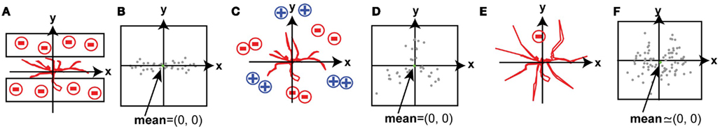
Figure 1. Spatial displacements of branch tips over time. Examples of instructed growth of neurites, in which the mean of the displacement vectors of individual neurites does not reveal the presence of directional instructive signals. (A,C,E) Schematic drawings that show representative experimental contexts in which growth inhibitory cues are presented in a stripe assay (A) or in discreet zones (C,E), where growth inhibition and growth promotion are represented by negative and positive signs, respectively. (B,D,F) Spatial representations of branch tip displacements, plotted as vectors of the change in branch tip positions induced by the experimental conditions in (A,C,E) respectively, plotted on an x,y coordinate, where the origin (0,0) indicates no displacement. (B) Shows displacements along the x axis, but little change along the y axis under conditions in which extending neurites are sandwiched by repellents. The spatial map in (C) shows displacements of individual branch tips in three directions, but no mean directional change, in response to a complex distribution of growth promoting and growth inhibiting cues. (E) Shows avoidance of a small sub-region, but very small mean directional change.

Materials and Methods

All experimental protocols were approved by the IACUC committees of Cold Spring Harbor Laboratory and The Scripps Research Institute, and complied with the guidelines established in the Public Health Service Guide for the Care and Use of Laboratory Animals.

Tadpole Preparation

Albino Xenopus laevis tadpoles were obtained either by matings of frogs from our colony or commercially from Nasco (Fort Atkinson, WI, USA). All tadpoles were reared in a 12-h light/12-h dark cycle incubator at 22°C. Retinotectal axons were labeled by expression of tdTomato as follows: Stage 41 tadpoles were anesthetized in 0.01% MS-222 (Sigma) solution and placed on an electrically grounded moist Kimwipe. Two plasmids pCMV:GAL4 and pUAS:TdTomato (final concentrations: 0.5 μg/μl) were mixed and pressure injected from a micropipette inserted between the retina and lens, using a picospritzer (Picospritzer II, General Valve Corporation). Fast Green (0.01%) was added to the DNA solution to monitor the injection into the eye. The pipette tip was placed close to the center of the retina and cells were electroporated by applying three 37 V pulses of 1.6 ms. Animals were screened under an epifluorescence microscope for successful labeling after 3 days.

In vivo Imaging

The animals were anesthetized in a 0.01% solution of MS-222 in 10% Steinberg’s solution. The anesthetized animals were mounted on a Sylgard support and imaged with a Perkin Elmer spinning disk confocal microscope. The samples were scanned over 336 μm × 336 μm × 180 μm (Z dimension). Images were collected once a day for 2 days.

Statistics

We present a general method that can be applied to several different biological situations. The specific statistical tests are selected according to the hypothesis to be tested and properties of the data. If the samples are independent, normally distributed, and the number of samples is large enough (typically ≥ 30), parametric tests, such as the paired t-test may be applicable. The statistical analysis requires that p-values be determined for the changes in length between each branch tip and each pixel in the map. Because identical statistical tests must be conducted for all of the pixels on the map, parametric statistical methods requiring that the data be normally distributed and independent probably cannot be used, because these conditions may not be satisfied for all the pixels. If these conditions are not met, then several options are available: pre-processing, for instance by applying the Box Cox transformation, can normalize the data and reduce the variance. Applying bootstrapping to the data is ideal because it does not depend on the fitting the data to known distributions. Alternately, a non-parametric test, such as the Wilcoxon signed-rank test or the Mann–Whitney U test can be used. Here, we used bootstrap tests to determine statistical significance of experimental data and examples in Figure 4 in which the data are not normally distributed. To make contour lines of p-values, maps of p-values are generated and lines joining pixels of similar p-values are superimposed on the color map. For the contour lines of p-values calculated by bootstrap tests, we used 1000 repetitions for each pixel and smoothed the map of p-values using a Gaussian filter (σ = 3) before making the contour lines. Increasing the number of bootstrap repetitions makes the maps of p-values more continuous.

Software

The software programs to make the displacement maps and the displacement vector maps are available at http://www.scripps.edu/research/faculty/cline.

Results

Directional Growth of Neuronal Branches

We were interested in establishing a method to assess complex structural rearrangements in response to global guidance cues, such as those underlying formation and plasticity of retinotopic maps or sensory representations in the cortex (Reh and Constantine-Paton, 1984; Sakaguchi and Murphey, 1985; Hickmott and Steen, 2005; De Paola et al., 2006; Bruno et al., 2009; Marik et al., 2010). An essential requirement of the analysis is that the analysis maintains spatial information pertaining to individual branches within a neuronal arbor in the context of the field or environment in which the branch rearrangements are occurring. In many quantitative analyses, the dynamic behaviors of multiple branches are integrated into a single value, such as an average, however, this simplification loses information about the distribution of cues embedded in the environment. To solve this problem, we analyze branch dynamics over time and present data as displacement vectors superimposed on a map of the growth field. This application of the method addresses the loss of spatial information caused by averaging the displacements of individual branches (Figures 1B,D,F) and detects the direction of movement of the population of branches. The principle advantage of this application of the method is that it preserves information about the magnitude and direction of branch dynamics within a growth field when the data from individual branches in many neuronal arbors are integrated.

We started by analyzing the displacements of Xenopus retinotectal axon branches as the arbors grow into the optic tectum. Two confocal images of individual retinotectal axon arbors were collected in vivo over a 24-h interval. Three-dimensional reconstructions of the axon arbors were made from the confocal z-stacks using the “trace filaments” module in IMARIS (Bitplane) and the data were exported as text files. Reconstructions are displayed as filament drawings for each time point (Figure 2A). Next, the filaments were aligned (Figure 2B). The alignment yields the offset values of rotation and shift for the entire filament reconstructions in x, y, and z. We wrote a MATLAB script to display and align the filaments. The text file from IMARIS is imported into MATLAB and the skeletons of the two axon arbors are coarsely aligned manually. Next, the entire data sets of the two filament reconstructions are aligned by the iterative closest point method. The coarse alignment is sometimes necessary because the iterative closest point method alone cannot correct large misalignments because it searches for a local closest point. Next, branch points of corresponding branches from the two time points are aligned, and the spatial displacement of the branch tips is calculated. The displacements of branch tips are displayed in Figure 2C. For this example of displacements of retinotectal axon branches, the filament drawings were flattened, so the data are evaluated in the x,y plane, because retinal axons are relatively flat in vivo (O’Rourke et al., 1994). Although this simplification of the data set sped up the computational time, the analysis can be done with three-dimensional data sets. A map that represents the branch rearrangements for all branches in the arbor is made by the following procedures, shown in Figures 2D–I. A single branch tip is selected and an x,y coordinate grid, that represents the imaged field, is superimposed on the aligned filament reconstructions so that the origin of the coordinate grid matches the position of the branch tip at the earlier time point (Figures 2D,E). This process is carried out by subtracting the x,y values of the position of the branch tip at the first time point, so the new values are 0,0 and the position of the branch tip at the second time point shows the direction and magnitude of the displacement of the branch tip over time. Then, the distances between each pixel on the grid and the branch tip at Day 1 and Day 2 are calculated (Figure 2E, l₀ and l) and these values are subtracted. This yields a three-dimensional displacement vector describing the displacement of the branch tip over the imaging interval. The first two dimensions describe the position of the branch tip at the second time point compared to first time point and are displayed as the position of the branch tip on the coordinate grid. The third dimension of the vector indicates the magnitude of the displacement, and is displayed in the color map. If the value is positive, the branch tip moved away from that location in the map; if the value is negative, the branch tip moved toward that location in the map. This process is repeated for each pixel on the grid (Figure 2F) and generates a displacement vector map that represents the displacement vectors between the single branch tip and all of the pixels in the imaged field (Figure 2G). The map is displayed in color code, in which warm colors (red–orange) indicate positions of vectors with positive changes in length, from which the branch retracted, and cool colors (blue–green) indicate positions of vectors with negative changes in length, toward which the branch extended. In other words, the map shows that the branch extended toward the relative positions marked by blue–green pixels and retracted from the relative positions marked by the red–orange pixels. The color map represents the spatial and dynamic information of the branch. Furthermore, by summing the displacement vector maps calculated from data from all branch tips in the arbor (Figure 2H), the features of the net branch movements for the arbor are integrated and presented in a color map (Figure 2I). The displacement vectors are normalized by the value at the coordinate origin, which corresponds to the sum of the displacements of all branch tips. Finally, displacement vector maps from multiple arbors in a data set are calculated and summed (Figures 2J,K).

FIGURE 2

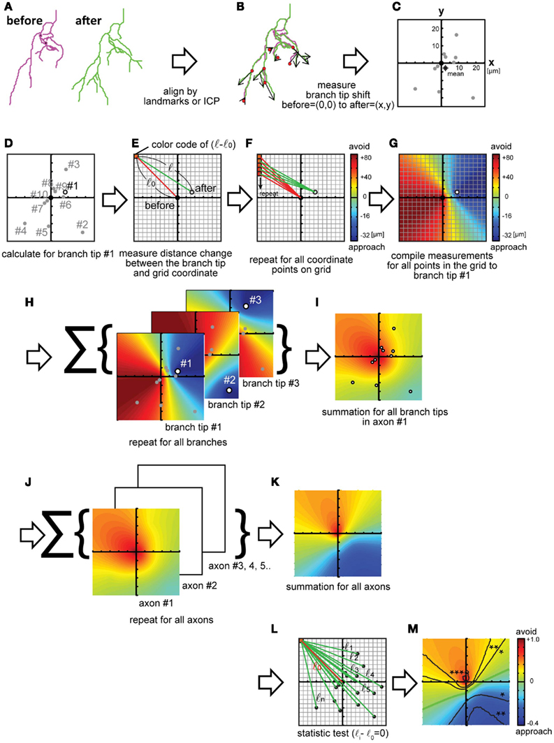
Figure 2. Calculations to generate a displacement maps. (A) Traced three-dimensional filament data at different time points are aligned by landmarks in the tissue or by cellular morphology, followed by an iterative closest point (ICP) algorithm. (B,C) Displacement vectors for each branch tip were calculated (B) and plotted on an x,y coordinate map (C). The origin represents no change in branch tip position. Star: the mean of all displacement vectors. (D–G) Calculation of changes in position for one of the branch tips [(D) circle, marked #1] relative to each pixel in the coordinate. One of the pixels is shown [(E): red]. Changes in branch tip distances in the spatial map are calculated by subtracting the distance between each pixel (red box) and the origin, the position of the branch tip at Day 1 (before: red line = l₀) from the distance between the same pixel position and the x,y location of the branch tip on Day 2 (after: green line = l). l − l₀ Represents the shift of the branch tip relative to the pixel (E). (F,G) A displacement vector map is generated by calculating displacement values for each branch tip for all pixels in the coordinate. Red–orange colors represent regions from which the branch retracted and blue–green colors show regions into which the branch extended (l − l₀ are negative values) (F). Next, maps are generated for all branch tips by iterating the calculations schematized in (E–H). The maps are summed (I). Displacement vector maps were calculated (J) for multiple axon arbors and summed (K). The significance of the distance change was tested using bootstrap methods (L). (M) Contour lines of p-values are superimposed on the map, as follows: *p < 0.05, **p < 0.01, ***p < 0.001, n = 82. Green line: displacement = 0. Maps are 336 μm on each side (J–M).

To provide a statistical analysis of the displacement vector maps, we generate contour lines signifying different p-values (Figure 2L) and superimpose the contour lines for relevant p-value on the maps (Figure 2M). In this application of the method, the null hypothesis is that branch tips do not move over the time interval studied. To make the contour lines of the p-values, the same statistical test needs to be used to assess the displacement vectors for each branch tip and each pixel in the map. Since it is unlikely that the data are normally distributed and independent for each pixel, we use bootstrapping to calculate p-values. First, a p-value is calculated for the change in lengths from each pixel to each branch tip at the two time points, and this is repeated for all pixels and all branches within an arbor (Figure 2L: l_{(i − j)} − l₀). Next, p-values are calculated for all pixels for all arbors and contour lines joining pixels of similar p-values are generated and superimposed on the color map (Figure 2M). We show the contour line for p < 0.05 on the map. The regions in the map where displacement vectors, i.e., pixels, are surrounded by the contour lines indicate the vectors with which the branch tips shifts consistently. Displacement vectors designating avoidance and approach are represented in red/orange and blue/green colors on the map, respectively.

The displacement vector map is a spatial representation of the integrated movement of all axon branches between two time points. Figure 3 shows several models of branch displacements along with the displacement vector maps and contour lines for p-values corresponding to the modeled branch dynamic data. If the movement of branches is spatially biased, the displacement vector map exhibits asymmetry with respect to the origin. If the movement is random, the displacement vector map is symmetric. The shape and distribution of the colors in the map and p-value contour lines provide more detailed information about the branch dynamics: If branches move uniformly in a specific direction (Figure 3A), which can happen when the branches are guided by a straight gradient of guidance cues, the color map shows steeper color changes close to the origin and the color changes form relatively straight lines in the map (Figure 3B). If the gradient of the guidance cue is curved (Figure 3C) or branches extend away from a focal point in the tissue (Figure 3D), the changes in the colors are relatively curved (Figure 3E).

FIGURE 3

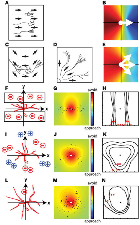
Figure 3. Spatial maps of virtual growth patterns. Simplified conditions in which all of the branches are guided by linear gradients of guidance cues (A,B) and cues distributed in non-linear patterns (C–E). If branches move in the same directions due to the linear gradient of cues (A), the steepness of the changes in the color representation of displacements is greater and form relatively straight lines (B). If the gradient of the guidance cue is curved (C) or branches extend away from a focal point in the tissue (D), the changes in color are curved in the map (E). (F–N) Displacement vector maps of the virtual situations in Figures 1A,C,E in which the mean of the displacement vectors did not provide directional information. Contour lines of p-values are shown as follows: *p < 0.05, **p < 0.01, ***p < 0.001. When neurites grow in a small stripe (F), the displacement vector map and the p-values represent contour lines surrounding a hot color region perpendicular to the restricted directions of growth (G,H). This map indicates that the movement of branches is more restricted along the vertical axis than horizontal axis. Spatial information can also be extracted when the growth of neurites is point symmetric (I–K) or when branches avoid a small region in the tissue (L–N). The asymmetric shape of the contour line shows the spatial asymmetry of the avoidance movements.

Displacement vector maps reveal directed growth of branches in situations in which simple vector summations cannot reveal directional movement (Figures 1A–D). For instance, when branch growth is limited to a small stripe (Figure 3F), the displacement vector map (Figure 3G) shows directional extension of branch tips and the p-value contour lines are perpendicular to the hemmed directions (Figure 3H), which means that the avoided regions are at the top and bottom of the map. Similarly, the displacement vector map reveals the regions in the growth field that are avoided when the branches extend in multiple directions from a symmetrical point (Figures 3I–K, compare with Figures 1C,D). This method can also reveal localized repulsive regions surrounded by non-instructive regions that allow random motion of branches (Figures 3L–N, compare with Figures 1E,F). The displacement vector maps preserve these spatial features of branch dynamics because the calculations are made in the context of the field in which the branches grow.

Identification of Attractive or Repulsive Regions in a Growth Field

The application of the method described above is optimal to test for responses to global growth cues, for instance when axons navigate in gradients of guidance signals, such as during topographic map formation. However, the method in Figure 2 is not optimal to detect the location of focal attractive or repulsive growth signals that are close to the growing neurites because such a signal can result in branches growing in many different directions. Consequently we developed methods which are designed to test whether local sources of attractive or repulsive cues are present in the growth field that can be detected by the growth response of neurites. The difference between this application of the method and the one described in Figures 2 and 3 is that generation of the displacement vector maps in Figure 2 requires that the branch positions of the earlier time point be aligned to the origin of the coordinate to provide information on relative changes in branch growth direction and magnitude between time points. By contrast, the branch positions of the earlier time point are not aligned to a common point and the changes in distance from all of the branch tips to each point in the actual tissue are calculated to generate a simple displacement map. This version of calculating the displacement map is useful to quantify redistributions of axon arbors, axon fasciculation, and tiling or territory of dendritic or axonal arbors, as described in the next three sections.

Redistribution of axon arbors over time

Axon arbors show significant changes in their location and morphology within target regions over time, which could occur in response to global or local growth cues. If the analysis described in Figure 2 does not indicate the presence of globally distributed growth signals, the application of the method described in Figures 4A,B can be used to test for local sources of attractive or repulsive signals within the growth field. Figure 4A shows an example of a retinotectal axon arbor from Xenopus tadpoles that undergoes a morphological change over a 2-day period of imaging. To determine the locations of regions that branch tips approach or avoid, we compare the sums of the distances from all branch tips in the arbor to each pixel in the growth field from the two time points, and plot the values as a displacement map. First, filament drawings from the two time points are aligned as described in the previous section. Next, for each pixel on the map, the distances from all of the branch tips to the pixel are calculated for the arbors at the two time points (Figure 4A, Σl_i and Σl_0i). The change in the total distance between the time points (Figure 4A, Σl_i − Σl_0i) is the value of displacement at the pixel. The value at each pixel is color coded on a map to indicate the distance change over the imaging interval (Figure 4B). In the displacement map (Figure 4B), actual positions that branches approach are indicated with cold colors and actual positions that branches avoid are indicated with hot colors. The null hypothesis is that the distance between pixels on the map and branch tips do not change over time. The same considerations for choice of the statistical test as mentioned above apply to this example. The significance of the differences in the distance (Figure 4A, Σl_i and Σl_0i) is tested for each pixel, and as described above, contour lines joining pixels of similar p-values are overlaid on the map.

FIGURE 4

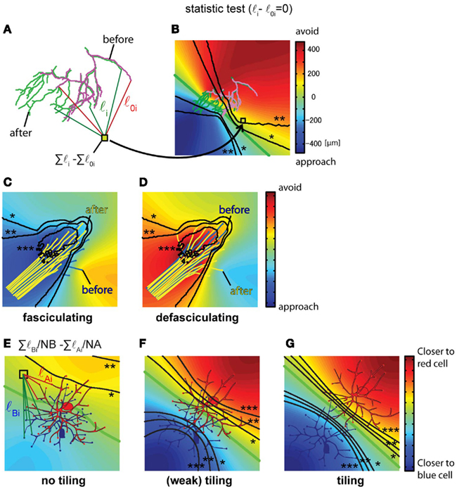
Figure 4. Identification of specific attractive/repulsive regions, axon fasciculation and detection of dendritic arbor tiling. (A,B) The absolute position of attractive or repulsive regions within a growth field is calculated for a Xenopus retinotectal axon arbor imaged twice over a 24-h interval. The arbor on Day 1 is magenta and on Day 2 is green. (A) First, the distances between the absolute positions of all branch tips on Day 1 and Day 2 and each pixel on the image were calculated, shown as l₀ for Day 1 data and l for Day 2 data, for all branches 1 through n. Next, the change in summed distances between the time points was calculated (Σl_i − Σl_0i). (When a new branch emerges, the branch point of the new branch is substituted into the branch tip position of the earlier time point.) (B) Identification of arbor territories of axons at different time points. The distance change (Σl_i − Σl_0i) is calculated for all of the pixels and values are color coded and superimposed on a map. p-Values are calculated for each pixel using bootstrapping (n = 33) and contour lines joining pixels of similar p-values are superimposed on the color maps. Displacement maps combined with the p-value contour lines indicate the regions which growth cones or branch tips significantly approach or avoid (*0.05, **0.01, ***0.001). (C,D) The same procedure can be used to distinguish the state of axon fasciculation, as shown in these drawings of virtual data. When axons fasciculate, cold colors appear in the central position of the axon bundle, indicating that axon branches approach the main axon bundle (C). When axons defasciculate, the axon bundle is embedded in warm colors, indicating the axons grow away from the fascicle (D). p-Value contour lines, *0.05, **0.01, ***0.001 (E–G). Quantification of dendritic tiling in three virtual cases showing different degrees of tiling superimposed on a displacement map. The formula, Σl_Bi/N_B − Σl_Ai/N_A, calculates the value for each pixel on the image corresponding to the sum of the distances from the pixel to each branch tip for the dendritic arbors of the blue and red neurons. N_A and N_B correspond to the number of dendritic branch tips in the red and blue neurons, respectively. The color map indicates the relative distance from each pixel to the dendrites of the red neuron and the blue neuron; hot colors indicate that branches are closer to the red neuron, cold colors indicate that branches are closer to the blue neuron. The green contour line is equidistant between the dendrites of the two neurons. The statistical significance of the difference between l_{A(i − j)}/N_A and l_{B(i − j)}/N_B is tested using Welch’s t-test for each pixel. Contour lines show p-values of 0.05 (*), 0.01 (**) and 0.001 (***). (B): 1 pixel = 1 μm². Maps are 336 μm on each side.

When the distance between each branch tip and each pixel in the representation of the tissue is calculated and compared between time points, the displacement map represents the specific position in the tissue that branches approach or avoid (Figures 4A,B). If the distribution of guidance signals is directly transformed into the spatial rearrangements of branches, the displacement map will predict the distribution of the guidance signals in the growth field. Nevertheless, the calculated attractive region (“sink”) may not directly reflect the location the guidance molecules for several reasons. One is that branches may exhibit persistent directional growth. A second is that the dynamic rearrangements of filopodia can generate heterogeneity in the direction of neurite movement. A third is that the signal transduction events, such as amplification by calcium influx (Hong et al., 2000; Wang and Poo, 2005), can be variable. If there is a discrepancy between the distribution of molecules of interest and the “sink,” or directed growth of neurites reported by the displacement map, this would suggest the participation of non-linear factors before or after recognition of the guidance molecules.

Fasciculation of axon bundles

Axon fasciculation is an important event in brain formation. Axon fasciculation forms axon tracts and plays a role in pathway selection by axons (Raper et al., 1983b). Spatially ordered axon fascicles are a structural basis of functional circuit modules (Senti et al., 2003). Some axon tracts are subdivided by different molecular mechanisms (Rajagopalan et al., 2000; Simpson et al., 2000; Wu et al., 2011), implying the presence of smaller functional modules in different groups of axons within a fascicle. Although it seems like a simple event, axon fasciculation is regulated by multiple mechanisms. It is induced by the cell autonomous function of molecules, such as Fasciclins (Bastiani et al., 1987; Lin et al., 1994), Semaphorins (Kolodkin et al., 1993), TAG-1 (Dodd et al., 1988), axonin-1, and ROBOs (Rajagopalan et al., 2000; Simpson et al., 2000). Non-cell autonomous signals, such as those downstream of axonin-1 (Ruegg et al., 1989) or BMP (Fu et al., 2006), also control fasciculation. These molecules can work in parallel, synergistically, or antagonistically. It is likely that many molecules and signaling cascades important for fasciculation remain to be discovered due to the complexity of the mechanisms controlling fasciculation.

The displacement map for the identification of attractive or repulsive regions in a growth field is also useful to identify and quantify mechanisms controlling fasciculation or defasciculation. To demonstrate this application of calculating the displacement map, the method described in Section “Redistribution of Axon Arbors Over Time” is applied to two virtual data sets of axon fasciculation and defasciculation (Figures 4C,D). The null hypothesis is that the distance between pixels on the map and branch tips do not change. The sum of distances from each pixel on the map to the axon tips at the two time points is determined, comparable to that shown in Figure 4A Σl_i and Σl_0i, and the difference (Σl_i − Σl_0i) for each pixel is color coded on a map to indicate the change in distance of the axon tips over the imaging interval (Figures 4C,D). The significance of the differences in the distance is statistically tested for each pixel using bootstrapping to establish statistical significance and contour lines joining pixels of similar p-values are overlaid on the map. When axons fasciculate, a common attractive region appears in the axon bundle (Figure 4C). On the other hand, when axons defasciculate, axons are repelled from a common region in the axon bundle (Figure 4D).

Tiling/territory of arbors

The positions of axonal or dendritic arbors and the degree of overlap of arbors influences neuronal connectivity. Dendritic tiling, which refers to the separation of dendritic arbor territories, is a topic of considerable interest in neuroscience (Tauchi and Masland, 1985; Jan and Jan, 2001; Grueber et al., 2002). For analysis of tiling of neuronal arbors, we assess three virtual data sets showing different degrees of tiling. The null hypothesis is that the arbors are overlapping. We quantify the overlap of the dendritic arbor territories using the formula Σl_Bi/N_B − Σl_Ai/N_A, as follows: the distances between each pixel on the map and all dendritic branch tips of the two cells, cell A and cell B, is determined, as Σl_Bi and Σl_Ai (Figure 4E). If the pixel on the map is closer to the arbor territory of cell A than to the arbor territory of cell B, then Σl_A will be less than Σl_B, and a map can be generated of the arbor territories based of the summed distances from each pixel to the branch tips of each arbor. If the arbor territories are calculated by mapping the differences of the sum of the distances, the cell with larger number of dendrites will have the larger calculated territory. Therefore, the sum of the distances is normalized by the number of branches in each cell, Σl_Bi/N_B and Σl_Ai/N_A, and the normalized values are subtracted, Σl_Bi/N_B − Σl_Ai/N_A. The values for each pixel are plotted on the map and color coded to indicate proximity of branches to cell A or cell B (Figures 4E–G). A green line marks the pixels that are equidistant between the branches of the two cells. When the two groups of dendritic branches are separated, two regions appear in which the sum of the distances between the pixels in that region and the branch tips are distinct, shown as the red and blue regions on the map. Statistical comparison of the differences in distances is determined for each pixel and pixels with similar p-values are joined in contour lines, as described above (Figures 4F,G: Welch’s t-test). A criterion to identify tiling is the presence of the two contour lines representing p = 0.05 located between the cell bodies of the two cells (Figures 4F,G, contour lines with *), which would indicate that branches are significantly closer to either cell A or B. Cells with strong tiling will have contour lines corresponding to p = 0.01 separating the cell bodies. For cells with overlapping dendritic arbors, the map will not show distinct regions indicating proximity of branches to either cell (Figure 4E) and the contour lines showing significance are not located between the cells.

Complex phenomena such as the establishment of dendritic arbor territories likely include contributions of multiple signaling pathways (Jan and Jan, 2001). We anticipate that this method for quantification of the relative overlap of arbor territories will be useful for the analysis of the signaling pathways and identification of the signaling components thought to control tiling, because it may be able to resolve partial effects on the phenotype that occur when individual signaling components are manipulated. Since this method not only evaluates territory formation but also represents spatial information, it may provide the opportunity to identify novel phenotypes in arbor dynamics and circuit development.

Discussion

We present an analytic method which represents multiple features of structural dynamics of neuronal axons or dendrites and arbor behavior in a spatial map. Since the method is simple, straightforward, and compatible with the frequently used analysis of displacement vectors or simple displacements, we expect it will be a versatile method to quantify and represent structural dynamics of neurons and glia in the context of their growth environment.

One strength of the method is its versatility. Several examples of modifications of the basic method are as follows. 1. While we presented the generation of two-dimensional displacement vector maps, three-dimensional maps can be made with the same method. The three-dimensional analysis will be useful to quantify axon or dendrite dynamics during the formation of laminar or columnar structures. 2. We describe a way to identify the presence of attractive or repulsive regions in a growth field. For this analysis, movements of all of the axon branches contributed equally to the values in the displacement map. To test the location of the cues more accurately, the current method could be used to simulate the location, range, and strength of the postulated guidance cue. 3. Here, branch tip positions are assessed in calculating the maps, however, the positions of other characteristic structures, such as postsynaptic sites, can be used depending on the hypothesized mechanism under analysis. Similarly, to calculate the displacement vector map or the displacement map, the change in distance (l) is calculated in the examples above, however, a function of distance, such as f(l), ln(l), or 1/(l) can be used, depending on the hypothesized distribution of guidance molecules in tissues or the behavior of neurites in response to guidance cues. 4. Finally, by focusing on the discrepancy between the actual location of the cues and the calculated attractive or repulsive regions, the presence of biological processes that are responsible for non-linearities in guidance mechanisms may be highlighted. For example, asymmetric, clockwise motions of filopodia, have been postulated to underlie the asymmetric structure of the brain (Tamada et al., 2010) through spatially biased response of axon arbors to the guidance cues. The comparison with the calculated location of the guidance cues and the actual cues will be helpful in revealing fundamental mechanisms in circuit formation. In conclusion, the method we present is applicable to multiple biological situations and may also be useful in multiple experimental circumstances.

Conflict of Interest Statement

The authors declare that the research was conducted in the absence of any commercial or financial relationships that could be construed as a potential conflict of interest.

Acknowledgments

We thank members of the Cline Lab for helpful discussions. Supported by the NIH (EY011261 and DP000458), the Nancy Marks Family Foundation, and endowments from the Marie and Charles Robertson Foundation and the Hahn Foundation to Hollis T. Cline.

References

Bastiani, M. J., du Lac, S., and Goodman, C. S. (1986). Guidance of neuronal growth cones in the grasshopper embryo. I. Recognition of a specific axonal pathway by the pCC neuron. J. Neurosci. 6, 3518–3531.

Pubmed Abstract | Pubmed Full Text

Bastiani, M. J., Harrelson, A. L., Snow, P. M., and Goodman, C. S. (1987). Expression of fasciclin I and II glycoproteins on subsets of axon pathways during neuronal development in the grasshopper. Cell 48, 745–755.

Pubmed Abstract | Pubmed Full Text | CrossRef Full Text

Bruno, R. M., Hahn, T. T., Wallace, D. J., de Kock, C. P., and Sakmann, B. (2009). Sensory experience alters specific branches of individual corticocortical axons during development. J. Neurosci. 29, 3172–3181.

Pubmed Abstract | Pubmed Full Text | CrossRef Full Text

de la Torre, J. R., Hopker, V. H., Ming, G. L., Poo, M. M., Tessier-Lavigne, M., Hemmati-Brivanlou, A., and Holt, C. E. (1997). Turning of retinal growth cones in a netrin-1 gradient mediated by the netrin receptor DCC. Neuron 19, 1211–1224.

Pubmed Abstract | Pubmed Full Text | CrossRef Full Text

De Paola, V., Holtmaat, A., Knott, G., Song, S., Wilbrecht, L., Caroni, P., and Svoboda, K. (2006). Cell type-specific structural plasticity of axonal branches and boutons in the adult neocortex. Neuron 49, 861–875.

Pubmed Abstract | Pubmed Full Text | CrossRef Full Text

Dodd, J., Morton, S. B., Karagogeos, D., Yamamoto, M., and Jessell, T. M. (1988). Spatial regulation of axonal glycoprotein expression on subsets of embryonic spinal neurons. Neuron 1, 105–116.

Pubmed Abstract | Pubmed Full Text | CrossRef Full Text

Flanagan, J. G., and Van Vactor, D. (1998). Through the looking glass: axon guidance at the midline choice point. Cell 92, 429–432.

Pubmed Abstract | Pubmed Full Text | CrossRef Full Text

Fu, M., Vohra, B. P., Wind, D., and Heuckeroth, R. O. (2006). BMP signaling regulates murine enteric nervous system precursor migration, neurite fasciculation, and patterning via altered Ncam1 polysialic acid addition. Dev. Biol. 299, 137–150.

Pubmed Abstract | Pubmed Full Text | CrossRef Full Text

Grueber, W. B., Jan, L. Y., and Jan, Y. N. (2002). Tiling of the Drosophila epidermis by multidendritic sensory neurons. Development 129, 2867–2878.

Pubmed Abstract | Pubmed Full Text

Hickmott, P. W., and Steen, P. A. (2005). Large-scale changes in dendritic structure during reorganization of adult somatosensory cortex. Nat. Neurosci. 8, 140–142.

Pubmed Abstract | Pubmed Full Text | CrossRef Full Text

Hong, K., Nishiyama, M., Henley, J., Tessier-Lavigne, M., and Poo, M. (2000). Calcium signalling in the guidance of nerve growth by netrin-1. Nature 403, 93–98.

Pubmed Abstract | Pubmed Full Text | CrossRef Full Text

Jan, Y. N., and Jan, L. Y. (2001). Dendrites. Genes Dev. 15, 2627–2641.

Pubmed Abstract | Pubmed Full Text | CrossRef Full Text

Kania, A., and Jessell, T. M. (2003). Topographic motor projections in the limb imposed by LIM homeodomain protein regulation of ephrin-A:EphA interactions. Neuron 38, 581–596.

Pubmed Abstract | Pubmed Full Text | CrossRef Full Text

Knoll, B., Weinl, C., Nordheim, A., and Bonhoeffer, F. (2007). Stripe assay to examine axonal guidance and cell migration. Nat. Protoc. 2, 1216–1224.

Pubmed Abstract | Pubmed Full Text | CrossRef Full Text

Kolodkin, A. L., Matthes, D. J., and Goodman, C. S. (1993). The semaphorin genes encode a family of transmembrane and secreted growth cone guidance molecules. Cell 75, 1389–1399.

Pubmed Abstract | Pubmed Full Text | CrossRef Full Text

Lance-Jones, C., and Landmesser, L. (1981). Pathway selection by chick lumbosacral motoneurons during normal development. Proc. R. Soc. Lond. B Biol. Sci. 214, 1–18.

Pubmed Abstract | Pubmed Full Text | CrossRef Full Text

Lin, D. M., Fetter, R. D., Kopczynski, C., Grenningloh, G., and Goodman, C. S. (1994). Genetic analysis of Fasciclin II in Drosophila: defasciculation, refasciculation, and altered fasciculation. Neuron 13, 1055–1069.

Pubmed Abstract | Pubmed Full Text | CrossRef Full Text

Marik, S. A., Yamahachi, H., McManus, J. N., Szabo, G., and Gilbert, C. D. (2010). Axonal dynamics of excitatory and inhibitory neurons in somatosensory cortex. PLoS Biol. 8, e1000395. doi: 10.1371/journal.pbio.1000395

Pubmed Abstract | Pubmed Full Text | CrossRef Full Text

Ming, G. L., Song, H. J., Berninger, B., Holt, C. E., Tessier-Lavigne, M., and Poo, M. M. (1997). cAMP-dependent growth cone guidance by netrin-1. Neuron 19, 1225–1235.

Pubmed Abstract | Pubmed Full Text | CrossRef Full Text

O’Rourke, N. A., Cline, H. T., and Fraser, S. E. (1994). Rapid remodeling of retinal arbors in the tectum with and without blockade of synaptic transmission. Neuron 12, 921–934.

Pubmed Abstract | Pubmed Full Text | CrossRef Full Text

Petros, T. J., Rebsam, A., and Mason, C. A. (2008). Retinal axon growth at the optic chiasm: to cross or not to cross. Annu. Rev. Neurosci. 31, 295–315.

Pubmed Abstract | Pubmed Full Text | CrossRef Full Text

Rajagopalan, S., Vivancos, V., Nicolas, E., and Dickson, B. J. (2000). Selecting a longitudinal pathway: robo receptors specify the lateral position of axons in the Drosophila CNS. Cell 103, 1033–1045.

Pubmed Abstract | Pubmed Full Text | CrossRef Full Text

Raper, J. A., Bastiani, M., and Goodman, C. S. (1983a). Pathfinding by neuronal growth cones in grasshopper embryos. I. Divergent choices made by the growth cones of sibling neurons. J. Neurosci. 3, 20–30.

Raper, J. A., Bastiani, M., and Goodman, C. S. (1983b). Pathfinding by neuronal growth cones in grasshopper embryos. II. Selective fasciculation onto specific axonal pathways. J. Neurosci. 3, 31–41.

Reh, T. A., and Constantine-Paton, M. (1984). Retinal ganglion cell terminals change their projection sites during larval development of Rana pipiens. J. Neurosci. 4, 442–457.

Pubmed Abstract | Pubmed Full Text

Ruegg, M. A., Stoeckli, E. T., Lanz, R. B., Streit, P., and Sonderegger, P. (1989). A homologue of the axonally secreted protein axonin-1 is an integral membrane protein of nerve fiber tracts involved in neurite fasciculation. J. Cell Biol. 109, 2363–2378.

Pubmed Abstract | Pubmed Full Text | CrossRef Full Text

Sakaguchi, D. S., and Murphey, R. K. (1985). Map formation in the developing Xenopus retinotectal system: an examination of ganglion cell terminal arborizations. J. Neurosci. 5, 3228–3245.

Pubmed Abstract | Pubmed Full Text

Senti, K. A., Usui, T., Boucke, K., Greber, U., Uemura, T., and Dickson, B. J. (2003). Flamingo regulates R8 axon-axon and axon-target interactions in the Drosophila visual system. Curr. Biol. 13, 828–832.

Pubmed Abstract | Pubmed Full Text | CrossRef Full Text

Simpson, J. H., Bland, K. S., Fetter, R. D., and Goodman, C. S. (2000). Short-range and long-range guidance by Slit and its Robo receptors: a combinatorial code of Robo receptors controls lateral position. Cell 103, 1019–1032.

Pubmed Abstract | Pubmed Full Text | CrossRef Full Text

Tamada, A., Kawase, S., Murakami, F., and Kamiguchi, H. (2010). Autonomous right-screw rotation of growth cone filopodia drives neurite turning. J. Cell Biol. 188, 429–441.

Pubmed Abstract | Pubmed Full Text | CrossRef Full Text

Tauchi, M., and Masland, R. H. (1985). Local order among the dendrites of an amacrine cell population. J. Neurosci. 5, 2494–2501.

Pubmed Abstract | Pubmed Full Text

Vactor, D. V., Sink, H., Fambrough, D., Tsoo, R., and Goodman, C. S. (1993). Genes that control neuromuscular specificity in Drosophila. Cell 73, 1137–1153.

Pubmed Abstract | Pubmed Full Text | CrossRef Full Text

Vielmetter, J., Stolze, B., Bonhoeffer, F., and Stuermer, C. A. (1990). In vitro assay to test differential substrate affinities of growing axons and migratory cells. Exp. Brain Res. 81, 283–287.

Pubmed Abstract | Pubmed Full Text | CrossRef Full Text

Walter, J., Kern-Veits, B., Huf, J., Stolze, B., and Bonhoeffer, F. (1987). Recognition of position-specific properties of tectal cell membranes by retinal axons in vitro. Development 101, 685–696.

Pubmed Abstract | Pubmed Full Text

Wang, G. X., and Poo, M. M. (2005). Requirement of TRPC channels in netrin-1-induced chemotropic turning of nerve growth cones. Nature 434, 898–904.

Pubmed Abstract | Pubmed Full Text | CrossRef Full Text

Wu, Z., Sweeney, L. B., Ayoob, J. C., Chak, K., Andreone, B. J., Ohyama, T., Kerr, R., Luo, L., Zlatic, M., and Kolodkin, A. L. (2011). A combinatorial semaphorin code instructs the initial steps of sensory circuit assembly in the Drosophila CNS. Neuron 70, 281–298.

Pubmed Abstract | Pubmed Full Text | CrossRef Full Text