Automatic reconstruction of neural morphologies with multi-scale tracking

Introduction

Revealing the structure of the neural circuits is an important challenge in neuroscience and could illuminate the understanding of their function. To document and measure the structure of neurons one traditionally uses manual reconstructions using a Camera Lucida or a computerized version of it. This time-tested method, however, is slow and laborious and it is common, even for a skilled researcher, to spend more than a week reconstructing the axonal arbor of a single neuron. This constitutes a significant bottleneck for the exploration of the structure of many neural circuits, particularly those, such as the neocortex, that could have many dozens of different cell types. Moreover, reconstructions of the same neuron by different researchers (or even by the same researcher) often differ, particularly when comparing the fine axonal branches (Yuste laboratory, unpublished observations).

The introduction of novel imaging techniques has opened the way for the design of automatic, or semi-automatic reconstructing methods, using stacks of microscopic images (Vasilkoski and Stepanyants, 2009; Yuan et al., 2009; Donohue and Ascoli, 2011), which are often preprocessed (Lichtman and Denk, 2011; Lu, 2011; Svoboda, 2011). Several different types of automated methods have been developed for neuronal reconstructions (Donohue and Ascoli, 2011), using two types of algorithms: skeletonization-based and tracking-based (Vasilkoski and Stepanyants, 2009; Yuan et al., 2009). The first class of algorithms extracts neural skeletons from grayscale (Yuan et al., 2009) or binary images (Cesar et al., 1997; Falco et al., 2002; Janoos et al., 2008), for example, using active contour models (Schmitt et al., 2004). However, this requires prior knowledge from the user, who has to first define the location of start and end points and branching points. Tracking algorithms, on the other hand, do not require user input and recursively find points belonging to structure boundaries and centerlines (Can et al., 1999; Al-Kofahi et al., 2002), or apply graph-based methods, like D:Dijkstras:1959] with either local or global search procedures. As an example of a local procedure, Wang et al. (2007) developed a dynamic tracking algorithm in 3D space that traverses along the axonal path while evaluating local properties such as smoothness, proximity, and continuity. In contrast, Dijkstra-based global tracking methods normally find the shortest paths between characteristic points of neural skeleton, such as branching points, start, and end points (Peng et al., 2010). For example, Gonzalez et al. (2010) built a graph-based procedure to find paths between points of maximal local “dendriteness,” called anchor points, detected using 3D steerable filters. The topology of the structure was then captured by selecting the minimum-cost tree, spanning the subset of the anchor points. Finally, some global tracking procedures do not use graph-based procedures. For example, Srinivasan et al. (2010) proposed a novel algorithm for tracking axons that incorporates a diffusion-based method.

The accurate detection of branches is one of the larger difficulties in neuronal reconstructions. The majority of existing algorithms either focus entirely on tracking straight segments or treat branching points simply as the intersection of two or more straight segments (Wang et al., 2011). The importance of detecting branchpoints was emphasized in Al-Kofahi et al. (2008), who introduced a generalized likelihood ratio test, defined on a spatial neighborhood of each candidate point, in which likelihoods were computed using a ridge-detection approach. As an alternative, Vasilkoski and Stepanyants (2009) proposed a voxel-coded procedure, designed for de-noised and preprocessed images, in which centers of intensity of consecutively coded wave fronts that scan the structure are connected into a branch structure that corresponds to the coarse trace of neurite, before an active contour method is applied for further refinement. These branchpoints were defined as the centers of intensity of the front regions, further divided in subsequent steps.

Based on this earlier work, we have developed a novel algorithm to track neurons using a procedure that simultaneously detects branching regions (as opposed to branching points, see below). Our main contribution is to introduce multi-scale techniques, combining both local and global information, for automatic detection and separation of branches. Our algorithm does not rely on ridge information, requires only a single initialization by the user and appears robust on tests on noisy databases. One limitation is its poor results on highly overlapping neural processes, a general problem when using blurred images where processes that are very close to each other, seem to intersect.

Materials and Methods

Original Data Sets

The data sets used in this study come from the DIADEM challenge (Brown et al., 2011; Gillette et al., 2011), downloaded from http://www.diademchallenge.org/. Specifically, we used data from olfactory projection fibers, a neocortical layer 6 neuron, cerebellar climbing fibers and a hippocampal CA3 interneuron. All data sets were originally manually reconstructed in 3D into .SWC files.

Generating Synthetic Data Sets

A neural tracking method typically consists of a preprocessing module and a tracking module. Our focus was on using multi-scaling for automatic neural tracking. Because of this, we chose a synthetic data set, assumed to have been preprocessed. However, differently from Vasilkoski and Stepanyants (2009) we assumed that the image still contains noise (modeled as “salt and pepper” noise). In addition, we also evaluated it on unprocessed data sets. We directly followed the procedure described in Vasilkoski and Stepanyants (2009), except that we operated with intensity values in the range of [0, 255] rather than fluorescence values. Thus, we assigned to each volume voxel overlapping with the trace the intensity value I_N = 255 and to all other voxels the intensity I_B = 0, following the assumption that neurite fluorescence is uniformly distributed. The obtained function I(x, y, z) [where I(x⁰, y⁰, z⁰) is the intensity value at point (x⁰, y⁰, z⁰) of the volume] was then convolved with the Gaussian point spread function:

$\text{PSF}\left(x,y,z\right)=\frac{1}{{\left(2\pi \right)}^{\frac{3}{2}}{\sigma }_x{\sigma }_y{\sigma }_z}*exp\left(-\frac{x^2}{2{\sigma }_x^2}-\frac{y^2}{2{\sigma }_y^2}-\frac{z^2}{2{\sigma }_z^2}\right)$

with equal standard deviation σ_x = σ_y = σ_z = σ in all 3D, in order to simulate light scattering in the tissue and in the microscope. The convolution operation produced the expected photon counts in the image stack:

$\begin{array}{llll}& \mu \left(x,y,z\right)& & \\ & =\int \left[I\left(x^{\prime },y^{\prime },z^{\prime }\right)*\text{PSF}\left(x-x^{\prime },y-y^{\prime },z-z^{\prime }\right)\right]d{x}^{\prime }d{y}^{\prime }d{z}^{\prime }& & \end{array}$

The actual photon count n(x, y, z) was then randomly generated for each voxel from the corresponding Poisson distributions:

$P\left(n|x,y,z\right)=\frac{exp\left[-\mu \left(x,y,z\right)\right]\mu {\left(x,y,z\right)}^n}{n!}$

To compensate for holes inside the neurite structure, we binarized each frame with a 0 threshold and then applied morphological closure. The obtained result was multiplied by 255 and added back to the volume. This way voxels inside the neurite that had intensity value 0 were set to intensity value 255. This procedure however did not eliminate large loops such as those created by two separate branches that may touch. Finally, to simulate noisy conditions we added to each frame of the image “salt and pepper” noise (generated using Matlab function imnoise) of level d, where d stands for the fraction of voxels corrupted with noise. This type of noise is inherent to confocal and wide field microscopy imaging (http://www.olympusmicro.com/primer/digitalimaging/deconvolution/deconintro.html). We experimentally observed that a noise level d = 15–20% was the threshold above which a human expert finds manual reconstruction highly difficult or impossible (Figure 1). Thus we inferred realistic scenarios enabling human experts to make reconstruction as characterized by a noise level between 0 and 15–20%.

FIGURE 1

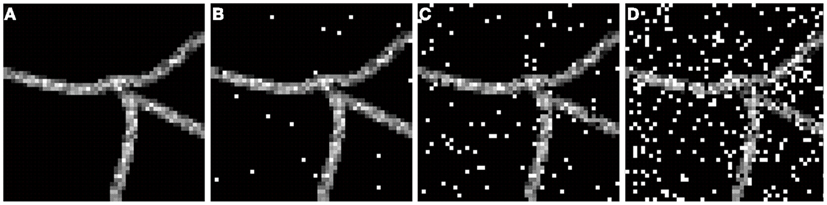
Figure 1. Exemplar frame showing fragment of neural structure corrupted with different levels of noise d: (A) d = 0, (B) d = 0.01, (C) d = 0.07, (D) d = 0.22.

Spanning Graph around the Seed Point

Figures 2 and 3 illustrate the process of tracking procedure described below. The algorithms starts tracking the neuron from a defined seed point. Let s⁰ be the seed point at time t = 0. This point is determined by the user and can be situated anywhere on the neural tree. A sphere of the radius R is then spanned around the seed point where R is also determined by the user. We empirically verified that choosing R to be const * σ where const range from 2 to 5 gave better results. Let V denotes the voxels within the sphere. We created a directed graph G = (V, E), where set V becomes the set of graph vertices and E is the set of graph edges. The edge between two vertices i and j is created if and only if the following conditions are satisfied:

FIGURE 2

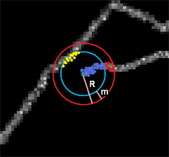
Figure 2. Spanning graph around a seed point. Graph consists of vertices connected to seed V_c (blue and red) and disconnected V_d (yellow). Subset of V_c are candidates (red) lying within a margin m from the surface of the sphere. Green point is the newly chosen seed point.

FIGURE 3

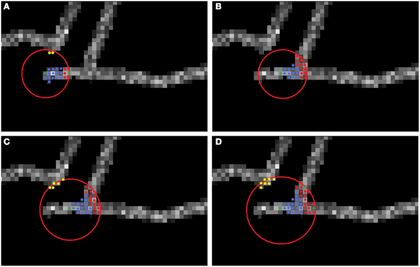
Figure 3. Multi-scaling procedure. The center of the sphere is the currently analyzed seed point (green). Graph vertices connected or disconnected from the seed point are respectively blue and yellow. (A) No branching detected. (B) First iteration of scaling. (C) Second iteration of scaling. (D) Last (in this case third) iteration of scaling. Green points from among the candidates (red) are the newly chosen seeds, starting from which each branch will be tracked.

$d_x{\left(i,j\right)}^2+d_y{\left(i,j\right)}^2\le 2\text{and}{d}_z\left(i,j\right)\le F_d$

where dx, dy, and dz are Euclidean distances respectively in x, y, and z between vertices and F_d is the distance in pixels between two consecutive frames of the volume, provided with the data set. The weight of the edge is determined as the weighted sum (this weight is then used to compute the length of Dijkstra path between any two vertices):

$c_1{d}_x\left(i,j\right)+c_2{d}_y\left(i,j\right)+c_3\frac{d_z\left(i,j\right)}{F_d}+c_4\frac{d_c\left(i\right)}{exp\left(1\right)}$

where $d_c\left(i\right)=\exp {\left(\frac{{}^I\max -I\left(i\right)}{I_{\max }}\right)}^2$, i is the voxel that is the head of the directed edge, I(i) is the intensity value of that voxel and I_max is the brightest intensity (and can be set to the brightest intensity in the sphere or in the entire volume). d_c capture how far the intensity of the target voxel (head of the directed edge) is from the brightest intensity.

Selecting New Seed Point in the Absence of Branching

The new selected seed point is chosen from among the set of candidates S_can defined as follows:

$\begin{array}{rcll}{S}_{\text{can}}& =\left\{v\in V_c:R^2\ge d_x{\left(v,s^t\right)}^2+d_y{\left(v,s^t\right)}^2\right.& & \\ & \left.+d_z{\left(v,s^t\right)}^2>{\left(R-m\right)}^2\right\}& & \end{array}$

where V_c consists of vertices connected to the seed, m denotes the margin such that the voxel within margin m from the sphere’s surface are all considered valid candidates, s^t denotes current seed point. The new seed point optimizes the objective function, that we call the point score, over each candidate point, s’, within S_can:

$\begin{array}{l}\text{score}\left(s^{\prime }\right)=g_1\frac{D\left(s^{\prime },s^t\right)-mi{n}_{s^{″}\in S_{can}}D\left(s^{″},s^t\right)}{ma{x}_{s^{″}\in S_{can}}D\left(s^{″},s^t\right)-mi{n}_{s^{″}\in S_{can}}D\left(s^{″},s^t\right)}\\ +\frac{g_2}{\pi }\arccos \frac{{\left(\left(s^t-s^{t-1}\right)\odot F_{vec}\right)}^T\left(\left(s^{\prime }-s^{t-1}\right)\odot F_{rev}\right)}{\parallel \left(s^t-s^{t-1}\right)\odot F_{vec}\parallel \cdot \parallel \left(s^{\prime }-s^{t-1}\right)\odot F_{rev}\parallel }\end{array}$

where $F_{vec}={\left[\begin{array}{c}\hfill 1\hfill \\ \hfill 1\hfill \\ \hfill F_d\hfill \end{array}\right]}^T$ is used to account for the different inter-voxel distance in different dimensions, g₁ and g₂ are coefficients determining the contribution of each term to the total score for the candidate point and D is the length of the Dijkstra path. ⊙ is the operand of the elementwise product between two vectors. The first term is the normalized weight of Dijkstra path from the candidate to the seed point and the second term is the normalized angle between the two vectors: the one from the previous seed point to the current one and the second one from the current seed point to the candidate point. In the first iteration the cosine of this angle is set to 1 for all candidates. The candidate chosen as the new seed point is the one with the minimal score.

While tracking the straight neural segment, we use the approach similar to Wang et al. (2007) where the global solution for the shortest path problem like Dijkstra’s algorithm whose computational complexity is at least O(E + V log V) is further simplified to the dynamic and local optimization problem with linear computational complexity.

Branching Detection and Multi-scaling

The algorithm then initialized a multi-scaling procedure. We defined the spread of points in the set P as:

$\text{spread}\left(P\right)=\text{ma}{\text{x}}_{\left(p_1,p_2\in p,p_1\ne p_2\right)}\frac{∥p_1-p_2∥}{R}$

and defined the branching region as the spherical region of radius R spanned around currently analyzed seed point for which spread (S_can) is above some threshold. In order to detect the branching region, the algorithm in each step analyses the normalized spatial spread of points in the set S_can, spread (S_can) by comparing it with the user-predefined threshold thr, typically in our experiments set to 2σ/R. If the normalized spatial spread is larger than the threshold, the algorithm enters the “danger” mode. In this mode the algorithm first decomposed S_can to a set of connected components (connected component is a set of voxels in S_can such that each voxel has at least one voxel from S_can in its 26-voxel neighborhood). Let CC_i denote ith connected component of S_can, let c_i be its voxel with the minimal point score and let K be the number of connected components found. The algorithm computes the spatial spread of each of the connected components. If at least one connected component has a spread larger than user-predefined value thr, the algorithm starts to scale the sphere. In each step the sphere radius is incremented by 1, the graph is rebuilt, and sets S_can and CC are recomputed. Scaling takes place until all connected components has spread smaller than the value of threshold thr or until the maximum number of scaling iterations iter_max was reached. The voxel c_i with minimal score of each connected component i ∈ K becomes new seed point in the corresponding connected component and ideally the new axon branch. Figure 3 illustrates the multi-scaling procedure. Since the branching possibly generates two new seed points, we keep the table of seed points STAB, from which we delete currently processed seed point while keeping all those that should be processed in the future.

Even if an expert manually reconstructs the neuron, the precise branching point location is still subjective to the expert judgment and may vary between experts. Thus, rather than the precise location of detecting branchpoints, we focused on regions of reasonable size parametrized by R, where branching is likely. Ideally, the true branch point and the seed point for which the scaling is initialized (interpreted as the branching point detected by our algorithm) should lie as close as possible and this indeed is often the case as shown in our experiments. The importance of multi-scaling is emphasized in Figure 4 where we show the unsatisfactory results of tracking exemplary neurons without applying multi-scaling.

FIGURE 4

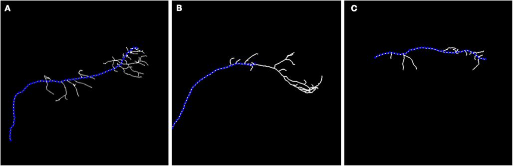
Figure 4. Maximum intensity projection image (MIP) of: olfactory projection fibers (A) OP1; (B) OP2; (C) OP3 with superimposed reconstruction. No multi-scaling was applied to obtain reconstructions.

Algorithm 1

INPUT: R, thr, STAB=[s0], itermax
while (STAB is non-empty)
  (1) s=the last element in table STAB
  remove s from STAB
  i=0
  (2) span the sphere of radius R around s
  build graph G(V, E)
  run Dijkstra algorithm
  select set of candidates Scan
  if (spread (Scan)(≤)thr)
   assign to each candidate a score
   choose $s=\arg {\min }_{s^{\prime }\in S_{can}}$ (score(s’))
   go to (2)
  else
   decompose Scan to a set of connected
   components {CC}
   if (∀i spread (CCi)<thr)
   STAB=STAB ∪ c1 ∪ c2 ∪ … ∪ cK
   go to (1)
   elseif (i ≤ itermax)
   R = R+1
   i = i+1
   go to (2)


Finally, we estimated the proximity between reconstructed and manual traces by computing the average and variance of the distance between the reconstructed points and their closest ground truth points. However, the provided ground truth datasets were not consistent in terms of the density of reconstructed points, since, in some cases, manually reconstructed points were densely located on the tree but in others there were significant sections without reconstruction points.

Results

We used synthetic data sets obtained from manual reconstructions from four different types of neurons: olfactory projection fibers (3 datasets), neocortical layer 6 axons (14 datasets), cerebellar climbing fibers (1 dataset), and hippocampal CA3 interneuron (14 datasets). The value of σ for the data generation was chosen to be the average radius of the structure computed from ground truth provided in .SWC files, and set it to 1 if the average was 0. Next we ran our algorithm on the data, with added salt and pepper noise of different density d where d represents the fraction of voxels corrupted with noise. We examined 10 different levels of noise [0, 0:01, 0:03, 0:05, 0:07, 0:09, 0:1, 0:15, 0:2, 0:22] and averaged the results over topologies obtained with noise levels: 0, 0.01, 0.03, 0.05, 0.07, 0.09, 0.1, and 0.15. Finally we tested our data on two “real” data sets, olfactory projection fibers: OP1 and OP3, that were slightly preprocessed. We employed several measures of the quality of obtained reconstructions: similarity factors, number of end points, length of automatic and manual reconstruction and precision, recall, and accuracy of the branching region detection. We additionally report the reconstruction time.

Similarity Factor

We generated two volumes: V_m, obtained from the ground truth .SWC file, and V_r, obtained from .SWC file with the tree reconstructed by our algorithm, using the following procedure. We reconstructed tree skeletons using linear interpolation between tree nodes (saved in .SWC files) and then blurred the obtained results using averaging filter of size 2σ + 1. The similarity factors are defined as:

$\begin{array}{rcll}& S_{\text{type}1}=\frac{\sum _{x,y,z}{V}_m\left(x,y,z\right)*V_r\left(x,y,z\right)}{\sum _{x,y,z}{V}_r\left(x,y,z\right)*V_r\left(x,y,z\right)}& & \\ & S_{\text{type}2}=\frac{\sum _{x,y,z}{V}_m\left(x,y,z\right)*V_r\left(x,y,z\right)}{\sum _{x,y,z}{V}_m\left(x,y,z\right)*V_m\left(x,y,z\right)}& & \end{array}$

Type 1 similarity measures how well reconstructed topology matches the ground truth topology and type 2 similarity measures how well ground truth topology matches the reconstructed one. Figure 5 shows the simple example of the planar behavior of similarity factors. The closer to 1 both factors are simultaneously, the more the reconstruction resembles the ground truth (notice however that factors can be either higher or lower than 1 but the perfect reconstruction achieves value 1 for both factors). Figure 6 shows the values of similarity factors for all data sets. On average the values of similarity factor type 1 was equal to 0.86 and the similarity factor type 2 was equal to 0.87. We noticed that both factors together capture well the level of consistency between ground truth topology and reconstructed topology. We empirically verified that the source of the majority of differences come from the fact that our algorithm occasionally misses very short branches or branch tips (of length less than R) as well as short branches located in the very close vicinity of much longer branches, due to the fact that the multi-scaling is performed until all branches are well separated. This limitation could be solved by terminating the multi-scaling process as soon as at least one branch is separated from others.

FIGURE 5

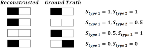
Figure 5. An example of the behavior of similarity factors (similarity factor type 1 S_{type 1} and similarity factor type 2 S_{type 2}) on simple planar example.

FIGURE 6

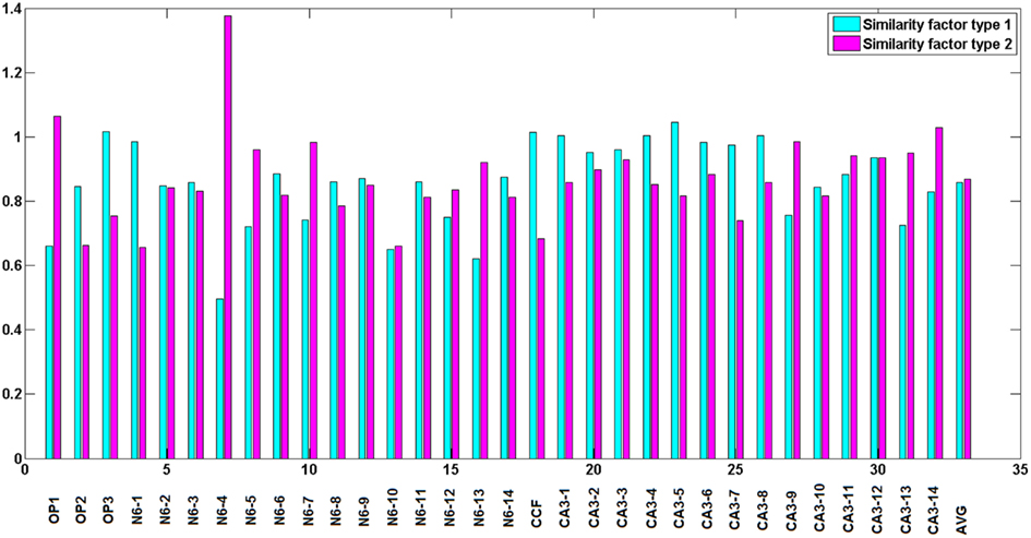
Figure 6. Similarity factors for all data sets, from left to right respectively: olfactory projection fibers: OP1, OP2, OP3, neocortical layer 6 axons, cerebellar climbing fibers, and hippocampal CA3 interneuron. The results are averaged over the topologies obtained with noise levels: 0, 0.01, 0.03, 0.05, 0.07, 0.09, 0.1, and 0.15. Last two bars show average similarity factors over all datasets.

Number of End Points and Trace Length

Since we observed that our algorithm occasionally misses very short branches (of length less than R) as well as those located in the very close vicinity of much longer branches, we wanted to verify how this in practice affects the quality of reconstruction. We therefore compared the number of end points and the length of reconstructed and ground truth topology (Figure 7, following the approach in Vasilkoski and Stepanyants, 2009). In both cases we found very high correlation, 0.9355 and 0.9996, respectively. However, in some cases the difference between the number of endpoints was significant, as it is seen on Figure 7. Particularly for cerebellar climbing fibers, the data set containing the largest tree with 92 end points, the difference was as high as 40, although, surprisingly, the lengths differ slightly. We verified that the main reason of differences between the number of end points was that the synthetic trees contain loops. The algorithm usually split them into two that contributes by a factor of 2 to the total number of end points. We conjecture that this issue can be partly alleviated by loop elimination processes. But in any case, the reconstruction error such as loop splitting affects the tree topology only slightly as can be seen by high similarity factors (type 1: 1 and type 2: 0.7) or directly in Figure 8 showing the detected and ground truth reconstruction.

FIGURE 7

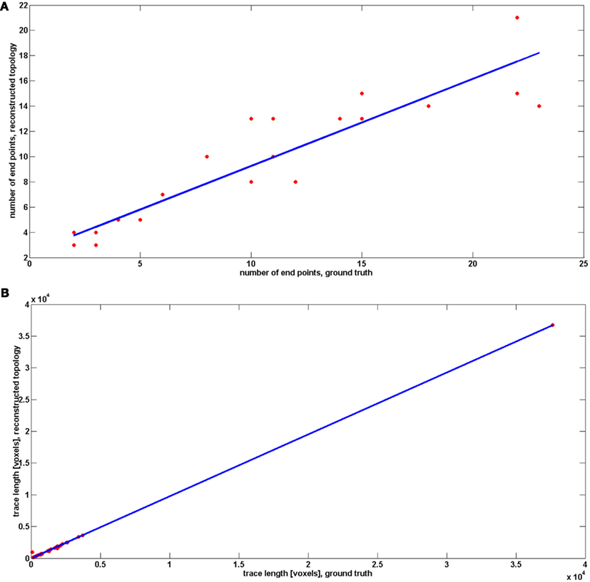
Figure 7. Comparison between number of end points (A) and traces length (B) between reconstructed topology and ground truth. The results for reconstructed topology are averaged over the topologies obtained with noise levels: 0, 0.01, 0.03, 0.05, 0.07, 0.09, 0.1, and 0.15.

FIGURE 8

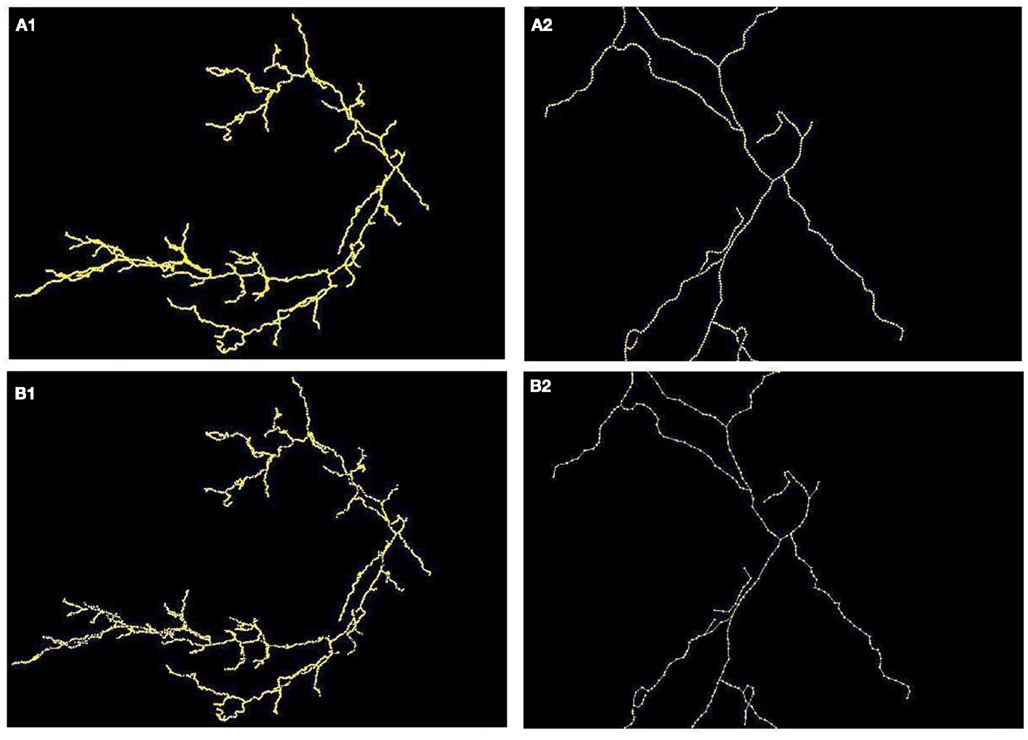
Figure 8. (A) Maximum intensity projection of cerebellar climbing fibers with superimposed reconstruction (A1) and zoomed fragment (A2). (B) Ground truth (B1) and (B2).

Precision, Recall, and Accuracy

To judge the quality of the detection of branching regions, we measured precision: $p=\frac{t_p}{t_p+f_p}$, recall: $r=\frac{t_p}{t_p+f_n},$ and accuracy: $a=\frac{t_p+t_n}{t_p+t_n+f_p+f_n}$, where t_p is the number of true positives or the number of correctly detected branching regions (the ones that contain true branching points; Figures 9A–C), t_n the number of true negatives (correct detection of non-branching regions), f_p the number of false positives (the ones that do not contain true branching points: Figure 9D), f_n the number of false negatives (missed branchings), and t_n the number or true negatives (correction detection of non-branching regions). t_p and f_p were computed by counting the number of seed points of the reconstructed topology for which the multi-scaling procedure was initialized, whose Euclidean distance to the closest true branching point is respectively no more than R (for t_p) or more than R (for f_p). t_n was set to 0 since we have no fair measure of proximity between our traces and the ground truth as it was mentioned in the end of section 2.5. f_n was computed by counting the number of branching points of the true topology, whose Euclidean distance to the closest seed point of reconstructed topology for which the multi-scaling procedure was initialized was more than R. Figure 10 shows the values of precision, recall, and accuracy for all data sets. The average precision obtained by our algorithm is 0.9, the average recall is 0.81 and the average accuracy is 0.75.

FIGURE 9

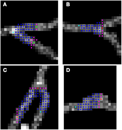
Figure 9. Possible situations when algorithm initialize multi-scaling: (A–C) true positives; (D) false positive (false alarm).

FIGURE 10

Figure 10. Precision, recall, and accuracy for all data sets, from left to right respectively: Olfactory projection fibers: OP1, OP2, OP3, neocortical layer 6 axons, cerebellar climbing fibers, and hippocampal CA3 interneuron. The results for reconstructed topology are averaged over the topologies obtained with noise levels: 0, 0.01, 0.03, 0.05, 0.07, 0.09, 0.1, and 0.15. Last two bars show average similarity factors.

In Figures 8, 11, and 12 we show the results of our tracking algorithm on most of the synthetic data sets we used in the study with noise level d = 0 (up to the level d = 0.15 the reconstructions were highly similar) and the ground truth for comparison. For neocortical layer 6 axons and hippocampal CA3 interneuron we show all trees on one MIP image, though each was reconstructed separately. We however also did tracked all trees in the same volume together. We followed the simple heuristics that no tree can split into more than two branches (detecting three branches indicates that two trees must have intersected and the algorithm chooses the middle branch since it is most probably the tree continuation). Finally, the performance of our algorithm measured using similarity factor, number of end points, trace length, precision, recall, or accuracy was still consistently satisfactory for noise level as high as d = 0.15, which represents a fairly noisy condition as shown in Figure 1.

FIGURE 11

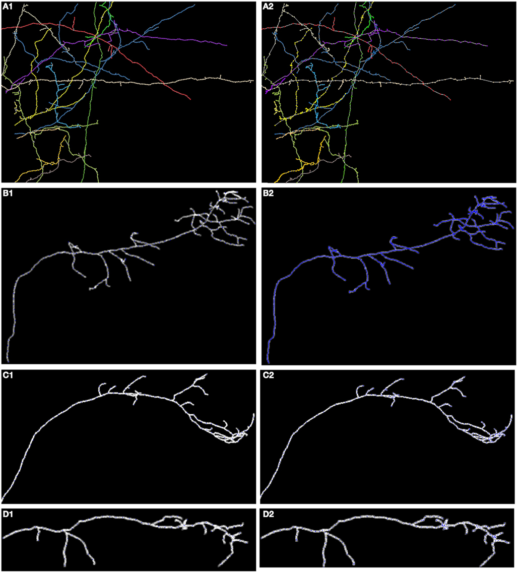
Figure 11. Maximum intensity projection of: (A) neocortical layer 6 axons; (B) olfactory projection fibers OP1; (C) OP2; (D) OP3; with superimposed reconstruction (A1–D1) and ground truth (A2–D2). Each color represents a different tree.

FIGURE 12

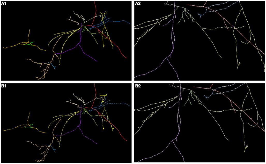
Figure 12. (A) Maximum intensity projection of hippocampal CA3 (each color represents a different tree; each tree was reconstructed separately) with superimposed reconstruction (A1) and zoomed fragment (A2). (B) Ground truth (B1) and (B2).

Reconstruction Time

Figure 13 shows the reconstruction time (CPU time in seconds) with respect to total length of neural topology (noise level 0) and number of end points (noise level also 0). We report the number of end points instead of the number of branches in order to be consistent with the analysis in Vasilkoski and Stepanyants (2009). Both the number of end points and trace length affect the tracking time, but the more end points, or the longer the structure is, does not necessarily requires more time to track the structure. In fact, we found that the most time-consuming step was the scaling, so all branching points that required multiple scaling contribute to the significant increase of the tracking time. The average reconstruction time for all data sets was 5 min, excluding cerebellar climbing fibers for which the reconstruction time was as high as 3.22 h. The program speed could be dramatically improved by optimizing the software implementation (for example, in a C/C++ environment). Finally, tracking time increased with noise level (Figure 13).

FIGURE 13

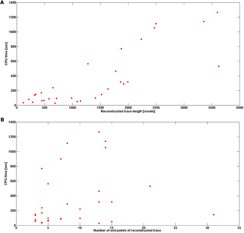
Figure 13. (A) Reconstruction time in seconds with respect to the length of reconstructed trace. (B) Reconstruction time in seconds with respect to the number of end points of reconstructed trace. The results are averaged over the topologies obtained with noise levels: 0, 0.01, 0.03, 0.05, 0.07, 0.09, 0.1, and 0.15.

Performance on Real Data Sets

We also performed experiments on real data sets (Figure 14). We chose olfactory projection fibers OP1 and OP3, fluorescence images that were de-noised using simple preprocessing tool, although we preserved the structure blurring. For each volume, we constructed a binary mask by thresholding each frame with an empirically determined threshold (0:035) and filtering it with median filter of size 5. We multiplied the original volume by the obtained 3D mask and applied a local thresholding step, dividing the volume into blocks of size 10 × 10 × 5 (in x, y, z respectively) and computing the mean m intensity in each of those blocks. We next set to 0 all voxels in each block whose intensity was lower than 0.8 * m. Next we applied our tracking algorithm (Table 1). The quality of reconstruction was worse than those for synthetic images, especially for OP1. For this data set the main challenge was the presence of many regions of densely packed branches due to poor preprocessing. For OP3, on the other hand, the overall performance is quite satisfactory. More advanced preprocessing could enable the algorithm to achieve higher performance for real data sets.

FIGURE 14

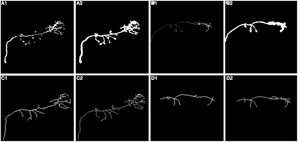
Figure 14. (A1,B1) Maximum intensity projection image (MIP) of olfactory projection fibers OP1 and OP3 respectively after preprocessing, (A2,B2) binarized MIP of OP1, OP3 respectively (C1,D1) Maximum Intensity Projection Image (MIP) of reconstructed topology of OP1, OP3, (C2,D2) Ground truth.

TABLE 1

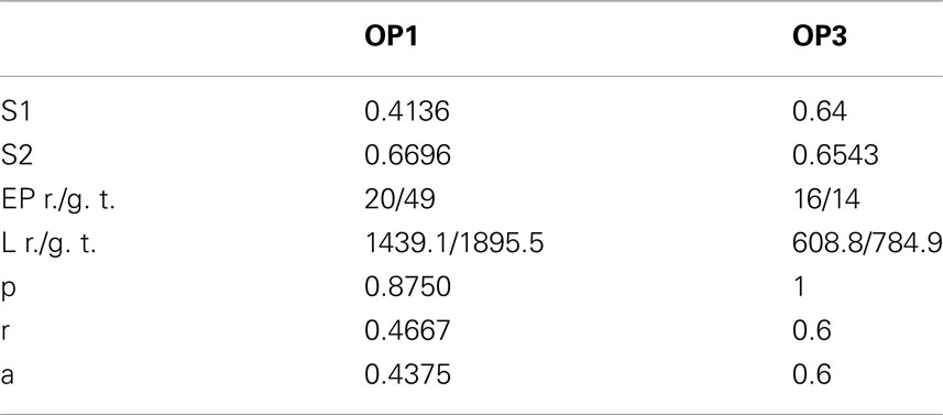
Table 1. Values of similarity factor type 1 (S1) and 2 (S2), number of end points for reconstructed topology/ground truth (EP), length in voxels of reconstructed topology/ground truth (L), precision (p), recall (r), and accuracy (a) in detecting branches for olfactory projection fibers OP1 and OP3.

Discussion

High-throughput, automatic 3D reconstructions of neuronal structures could enable a quantitative description of the structure of neural circuits. The use of image stacks has enabled the development of many novel methods for automatic reconstructions, some of which focus on image preprocessing to improve image quality, whereas others use tracking procedures to reveal the neurite topology. Most tracking algorithms either rely on ridge information (not suitable for blurred images) or on simplified assumptions, ignoring noise. Also, most tracking procedures do not explicitly address branch detection, but focus instead on relatively simple neural segments.

As an alternative, here we present a new algorithm for tracking the neural structure in 3D with simultaneous detection of branching regions that does not rely on edge information and is robust to the presence of noise in the image. Our method tolerates a noise level up to 15%, a level beyond which even trained human subjects may have difficulty performing manual reconstruction. Our algorithm achieved a promising performance (80–90% precision/recall) in detecting branching regions. The method combines some of the techniques previously used for 3D neural tracking with multi-scaling, a technique that originated in computer vision, that enables combination of both global and local image information. The obtained results indicate that our reconstructions are very similar to ground truth reconstruction generated by the human experts. Even though most reconstructions were performed on synthetic data, preliminary experiments suggest that it is possible to use the algorithm also for real data sets that are first preprocessed to remove the blurriness. It is also worth mentioning that it is not necessary to force the neuronal structure to be continuous after preprocessing since our method can be easily extended to handle small gaps in the structured to be traced, by modifying the local graph construction step.

In addition to the new algorithm, we have presented a comprehensive performance evaluation of synthetic data sets with controlled levels of noise based on a few well-defined metrics. Although there is no single best metric that can replace human judgments, some of our metrics are novel, such as similarity factors and sensitivity to noise.

One limitation of our algorithm is its poor results on highly overlapping neural processes, a general problem when using highly blurred images where processes that are very close or touch each other, seem to intersect. Distinguishing between bifurcations or crossings in such cases is confusing even for the experienced human operator (Senft, 2011) and, in fact, this is believed to be the hardest challenge in automated tracing (Lu et al., 2009; Ropireddy et al., 2011). To the best of our knowledge, existing reconstruction systems use manual feedback provided by a human expert to assist the computer algorithm in these ambiguity situations. Furthermore, in these cases, tracking is often preceded by several preprocessing steps (i.e., Luisi et al., 2011; Narayanaswamy et al., 2011; Ropireddy et al., 2011). The reason why tracking procedures performs poorly in these situations is because, on blurred images, close processes look like intersecting ones and blurred branches of a same process lying close tend to form loops. One solution could be to develop a preprocessing platform to reduce the amount of image blurriness and the number of loops. Finally, the lack of the determination of the precise branching location can be perceived as the second limitation of the algorithm. In future extension of this work, this problem could be solved by downscaling the sphere after the initial process of scaling to separate the branches.

In summary, our results indicate that multi-scaling is a promising approach for the automation and improvement of the quality of reconstruction of neural morphologies and should be investigated in more depth.

Conflict of Interest Statement

The authors declare that the research was conducted in the absence of any commercial or financial relationships that could be construed as a potential conflict of interest.

Acknowledgments

We thank Laura McGarry and anonymous reviewers for their valuable input.

References

Al-Kofahi, K. A., Lasek, S., Szarowski, D. H., Pace, C. J., Nagy, G., Turner, J. N., and Roysam, B. (2002). Rapid automated three-dimensional tracing of neurons from confocal image stacks. IEEE Trans. Inf. Technol. Biomed. 6, 171–187.

Pubmed Abstract | Pubmed Full Text | CrossRef Full Text

Al-Kofahi, Y., Dowell-Mesfin, N., Pace, C., Shain, W., Turner, J. N., and Roysam, B. (2008). Improved detection of branching points in algorithms for automated neuron tracing from 3D confocal images. Cytometry A 73A, 36–43.

CrossRef Full Text

Brown, K. M., Barrionuevo, G., Canty, A. J., De Paola, V., Hirsch, J. A., Jefferis, G. S. X. E., Lu, J., Snippe, M., Sugihara, I., and Ascoli, G. A. (2011). The DIADEM data sets: representative light microscopy images of neuronal morphology to advance automation of digital reconstructions. Neuroinformatics 9, 143–157.

Pubmed Abstract | Pubmed Full Text | CrossRef Full Text

Can, A., Shen, H., Turner, J. N., Tanenbaum, H. L., and Roysam, B. (1999). Rapid automated tracing and feature extraction from retinal fundus images using direct exploratory algorithms. IEEE Trans. Inf. Technol. Biomed. 3, 125–138.

Pubmed Abstract | Pubmed Full Text | CrossRef Full Text

Cesar, R. M., Da, L., and Costa, F. (1997). “Semi-automated dendrogram generation for neural shape analysis,” in Proceedings of the 10th Brazilian Symposium on Computer Graphics and Image Processing, Campos do Jordão, 147–154.

Dijkstra, E. W. (1959). A note on two problems in connexion with graphs. Numerische Mathematik 1, 269–271.

CrossRef Full Text

Donohue, D. E., and Ascoli, G. A. (2011). Automated reconstruction of neuronal morphology: an overview. Brain Res. Rev. 67, 94–102.

Pubmed Abstract | Pubmed Full Text | CrossRef Full Text

Falco, A. X., da Fontoura Costa, L., and da Cunha, B. S. (2002). Multiscale skeletons by image foresting transform and its application to neuromorphometry. Pattern Recognit. 35, 1571–1582.

CrossRef Full Text

Gillette, T. A., Brown, K. M., Svoboda, K., Liu, Y., and Ascoli, G. A. (2011). DIADEMchallenge.Org: a compendium of resources fostering the continuous development of automated neuronal reconstruction. Neuroinformatics 9, 303–304.

CrossRef Full Text

Gonzalez, G., Turetken, E., Fleuret, F., and Fua, P. (2010). “Delineating trees in noisy 2D images and 3D image stacks,” in Proceedings of the IEEE international conference on Computer Vision and Pattern Recognition, 2010, San Francisco.

Janoos, F., Nouansengsy, B., Xu, X., Machiraju, R., and Wong, S. T. C. (2008). Classification and uncertainty visualization of dendritic spines from optical microscopy imaging. Comput. Grap. Forum 27, 879–886.

CrossRef Full Text

Lichtman, J. W., and Denk, W. (2011). The big and the small: challenges of imaging the brain’s circuits. Science 334, 618–623.

Pubmed Abstract | Pubmed Full Text | CrossRef Full Text

Lu, J. (2011). Neuronal tracing for connectomic studies. Neuroinformatics 9, 159–166.

Pubmed Abstract | Pubmed Full Text | CrossRef Full Text

Lu, J., Fiala, J. C., and Lichtman, J. W. (2009). Semi-automated reconstruction of neural processes from large number of fluorescence images. PLoS ONE 4, e5655. doi:10.1371/journal.pone.0005655

CrossRef Full Text

Luisi, J., Narayanaswamy, A., Galbreath, Z., and Roysam, B. (2011). The FARSIGHT trace editor: an open source tool for 3-D inspection and efficient pattern analysis aided editing of automated neuronal reconstructions. Neuroinformatics 9, 305–315.

Pubmed Abstract | Pubmed Full Text | CrossRef Full Text

Narayanaswamy, A., Wang, Y., and Roysam, B. (2011). 3-D image pre-processing algorithms for improved automated tracing of neuronal arbors. Neuroinformatics 9, 247–261.

Pubmed Abstract | Pubmed Full Text | CrossRef Full Text

Peng, H., Ruan, Z., Long, F., Simpson, J. H., and Myers, E. W. (2010). V3D enables real-time 3D visualization and quantitative analysis of large-scale biological image data sets. Nat. Biotechnol. 28, 348–353.

Pubmed Abstract | Pubmed Full Text | CrossRef Full Text

Ropireddy, D., Scorcioni, R., Lasher, B., Buzsaki, G., and Ascoli, G. A. (2011). Axonal morphometry of hippocampal pyramidal neurons semi-automatically reconstructed after in vivo labeling in different CA2 locations. Brain Struct. Funct. 216, 1–15.

Pubmed Abstract | Pubmed Full Text | CrossRef Full Text

Schmitt, S., Evers, J. F., Duch, C., Scholz, M., and Obermayer, K. (2004). New methods for the computer-assisted 3-d reconstruction of neurons from confocal image stacks. Neuroimage 23, 1283–1298.

Pubmed Abstract | Pubmed Full Text | CrossRef Full Text

Senft, S. L. (2011). A brief history of neuronal reconstruction. Neuroinformatics 9, 119–128.

Pubmed Abstract | Pubmed Full Text | CrossRef Full Text

Srinivasan, R., Li, Q., Zhou, X., Lu, J., Lichtman, J., and Wong, S. T. C. (2010). Reconstruction of the neuromuscular junction connectome. Bioinformatics 26, 64–70.

CrossRef Full Text

Svoboda, K. (2011). The past, present, and future of single neuron reconstruction. Neuroinformatics 9, 97–98.

Pubmed Abstract | Pubmed Full Text | CrossRef Full Text

Vasilkoski, Z., and Stepanyants, A. (2009). Detection of the optimal neuron traces in confocal microscopy images. J. Neurosci. Methods 178, 197–204.

Pubmed Abstract | Pubmed Full Text | CrossRef Full Text

Wang, J., Zhou, X., Lu, J., Lichtman, J., Chang, S. F., and Wong, S. T. C. (2007). “Dynamic local tracing for 3d axon curvilinear structure detection from microscopic image stack,” in ISBI’07, Washington, 81–84.

Wang, Y., Narayanaswamy, A., Tsai, C.-L., and Roysam, B. (2011). A broadly applicable 3-D neuron tracing method based on open-curve snake. Neuroinformatics 9, 193–217.

Pubmed Abstract | Pubmed Full Text | CrossRef Full Text

Yuan, X., Trachtenberg, J., Potter, S., and Roysam, B. (2009). MDL constrained 3-D grayscale skeletonization algorithm for automated extraction of dendrites and spines from fluorescence confocal images. Neuroinformatics 7, 213–232.

Pubmed Abstract | Pubmed Full Text | CrossRef Full Text