Bayesian inference for generalized linear models for spiking neurons

Introduction

A common problem in system neuroscience is to understand how information about the sensory stimulus is encoded in sequences of action potentials (spikes) of sensory neurons. Given any stimulus, the goal is to predict the neural response as well as possible, as this can give insights into the computations carried out by the neural ensemble. To this end, we want to have flexible generative models of the neural responses which can still be fit to observed data. The difficulty in choosing a model is to find the right trade-off between flexibility and tractability. Adding more parameters or features to the model makes it more flexible but also harder to fit, as it is more prone to overfitting. The Bayesian framework allows one to control for the model complexity even if the model parameters are underconstrained by the data, as imposing a prior distribution over the parameters allows regularizing the fitting procedure (Lewicki and Olshausen, 1999 ; Ng, 2004 ; Steinke et al., 2007 ; Mineault et al., 2009 ).

From a statistical point of view, building a predictive model for neural responses constitutes a regression problem. Linear least squares regression is the simplest and most commonly used regression technique. It provides a unique set of regression parameters, but one that is derived under the assumption that neural responses in a time bin are Gaussian distributed. This assumption, however, is clearly not appropriate for the spiking nature of neural responses. Generalized Linear Models (GLMs) provide a flexible extension of ordinary least squares regression which allows one to describe the neural response as a point process (Brillinger, 1988 ; Chornoboy et al., 1988 ) without losing the possibility of finding a unique best fit to the data (McCullagh and Nelder, 1989 ; Paninski, 2004 ).

The simplest example of the generalized linear spiking neuron model is the linear-nonlinear Poisson (LNP) cascade model (Chichilnisky, 2001 ; Simoncelli et al., 2004 ). In this model, one first convolves the stimulus with a linear filter, subsequently transforms the resulting one-dimensional signal by a pointwise nonlinearity into a non-negative time-varying firing rate, and finally generates spikes according to an inhomogeneous Poisson process. Importantly, the GLM model is not limited to noisy Poisson spike generation: analogous to the stimulus signal, one can also convolve the recent history of the spike train with a feedback filter and transform the superposition of both stimulus and spike history filter outputs through the pointwise nonlinearity into an instantaneous firing rate in order to generate the spike output. In this way one can mimic dynamical properties such as bursts, refractory periods and rate adaptation. Finally, it is possible to add further input signals originating from the convolution of a filter kernel with spike trains generated by other neurons (Borisyuk et al., 1985 ; Brillinger, 1988 ; Chornoboy et al., 1988 ). This makes it possible to account for couplings between neurons, and to model data which exhibit so called noise correlations, i.e., correlations which can not be explained by shared stimulus selectivity. Although the GLM only gives a phenomenological description of the neurons’ properties, it has been shown to perform well for the prediction of spike trains in the retina (Pillow et al., 2005 , 2008 ), in the hippocampus (Harris et al., 2003 ) and in the motor cortex (Truccolo et al., 2010 ).

In this paper we seek to explore the potential uses and limitations of the framework for approximate Bayesian inference for GLMs based on the Expectation Propagation algorithm (Minka, 2001 ). With this framework, we can not only approximate the posterior mean but also the posterior covariance and hence compute confidence intervals for the inferred parameter values. Furthermore, the posterior mean is an alternative to the commonly used point estimators, maximum a posteriori (MAP) or maximum likelihood. Like the MAP also the posterior mean can be used with a Gaussian or a Laplacian prior leading to an L2 or an L1-norm regularization. To establish the approximate inference framework, we compare these point estimates on the basis of two different quality measures: prediction performance and filter reconstruction error. In addition, we investigate different binning schemes and their impact on the different inference procedures. Along with the paper we publish a MATLAB (the code is available at http://www.kyb.tuebingen.mpg.de/bethge/code/glmtoolbox/ ) toolbox in order to support researchers in the field to do Bayesian inference over the parameters of the GLM spiking neuron model.

The paper is organized as follows. In Section “Generalized Linear Modeling for Spiking Neurons”, we review the definition of the Generalized Linear Model and present the expansion into a high-dimensional feature space. We explain how a Laplace prior can improve the prediction performance in this setting and how different loss functions can be used to rate different quality aspects. In Section “Approximating the Posterior Distribution Using EP”, we present how the posterior distribution for observed data in the GLM setting can be approximated via the Expectation Propagation algorithm. Finally in Section “Potential Uses and Limitations” we systematically compare the MAP estimator to the posterior mean assuming Gaussian versus a Laplacian prior. In addition we apply the GLM framework to multi-electrode recordings from a population of retinal ganglion cells and discuss the potential differences of discretizing time directly or discretizing the features.

Generalized Linear Modeling for Spiking Neurons

Specifying the Likelihood

The Generalized Linear Model (GLM) of spiking neurons describes how a stimulus s(t) is encoded into a set of spike trains generated by neurons i = 1,…,N, j = 1,…,N_i (Brillinger, 1988 ; Chornoboy et al., 1988 ; Paninski, 2004 ; Okatan et al., 2005 ; Truccolo et al., 2005 ) (See Stevenson et al., 2008 for a recent review). More precisely, s(t) is a vector of dimensionality n, which describes the history of the stimulus signal up to time t according to a suitable parametrization. For example, in Section “Potential Uses and Limitations” where we apply the GLM to retinal ganglion cell data, the vector s(t) contains the light intensities of the full-field flicker stimulus for the last n frames up to time t. The GLM assumes that an observed spike train {t_j} is generated by a Poisson process with a time-varying rate λ(t). In its simplest form the rate λ(t) depends only on the stimulus vector s(t). This special case of the GLM is also known as the LNP model (Simoncelli et al., 2004 ). Specifically, the rate can be written as a Linear-Nonlinear cascade:

First, the stimulus is filtered with a linear filter w_s which is referred to as the receptive field of the neuron. Subsequently, the pointwise monotonic nonlinearity f transforms the real-valued output of the linear filtering into a non-negative instantaneous firing rate. If the current stimulus has a strong overlap with the receptive field, that is if s(t)^Tw_s is large, this will yield a large probability of firing. If it is strongly negative, the probability of firing will be zero or close to zero.

In the classical GLM framework (McCullagh and Nelder, 1989 ), f⁻¹ is also called “link function”. For the Poisson process noise model, the link function must be both convex and log-concave in order to preserve concavity of the log-posterior (Paninski, 2004 ). Thus it must grow at least linearly and at most exponentially. Typical choices of this nonlinearity are the exponential or a threshold linear function,

As the spikes are assumed to be generated by a Poisson process, the log-likelihood of observing a spike train {t_j} is given by

In this simple form, the GLM ignores some commonly observed properties of spike trains, such as refractory periods or bursting effects. In order to address this problem, we want to make the firing rate λ(t) dependent not only on the stimulus but also on the history of spikes generated by the neuron. To this purpose, an additional linear filtering term can be added into Eq. 1. For example, by convolving the spikes generated in the past with a negative-valued kernel, we can account for the refractory period. The instantaneous firing rate of the GLM then results from a superposition of two terms, a stimulus and a spike feedback term:

The m-dimensional vector ψ_h(t) describes the spiking history of the neuron up to time t according to a suitable parametrization. A simple parametrization is a spike histogram vector whose components contain the number of spikes in a set of preceding time windows. That is, the k-th component (ψ_h(t))_k contains the number of spikes in the time window (t − Δ_k+1, t − Δ_k] with The linear weights w_h can then be fit empirically to model the specific dynamic properties of the neuron such as its refractory period or bursting behavior. The encoding scheme is illustrated in Figure 1 .

FIGURE 1

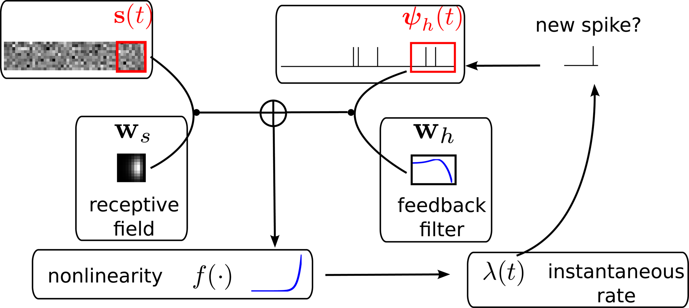
Figure 1. Illustration of the generative encoding model associated with a GLM: the stimulus s(t) as well as the spiking history ψ_h(t) are filtered with their corresponding receptive fields w_s and w_h. A nonlinearity f is applied to the sum of the outputs to produce an instantaneous rate, which then is used to generate new spikes.

Analogous to the spike feedback just described, the encoding can readily be extended to the population case, if the vector ψ_h(t) for each neuron not only describes its own spiking history, but includes the spiking history of all other neurons as well. Taken together, the log-likelihood of observing the spike times for a population of i = 1,…,N neurons is given by

Although the likelihood factorizes over different neurons i, this does not imply that the neurons fire independently. In fact, every neuron can affect any other neuron i via the spiking history term ψ_h(t). Thus, by fitting the weighting term to the data we can also infer effective couplings between the neurons.

In order to evaluate Eq. 4 we have to calculate the integral numerically. In terms of computation time, this easily becomes a dominating factor when the recording time T is large. Many artificial stimuli used for probing sensory neurons such as white noise can be described as piecewise constant functions. For example, the stimulus used for the retinal ganglion cells in Section “Population of Retinal Ganglion Cells” had a refresh rate of 180 Hz. In this case, the stimulus s(t) only changes at particular points in time. Further, if we use the spike histogram vector mentioned above to describe the spiking history of the neurons, then also ψ_h(τ) is a piecewise constant function. Thus, we can find time points τ₁,…,τ_z between which neither the stimulus nor the vector describing the spiking history changes. We call the τ_i “discretization-points”. Also in cases in which the features are not piecewise constant such a discretization can be approximately obtained in a data-dependent manner, which we show in Section “Data-Dependent Discretization of the Time-Axis”. By decomposing the integral over (0, T) into a sum of integrals over the intervals [τ_k, τ_k+1) within which the integrand stays constant, the log-likelihood can be simplified to:

Note that ψ_h(τ_k) and ψ_s(τ_k) are constant, since the features do not change in the interval [τ_k, τ_k+1).

Extending the Computational Power of GLMs

To increase the flexibility of a GLM, several extensions are possible. For example, one can add hidden variables (Kulkarni and Paninski, 2007 ; Nykamp, 2008 ) or weaken the Poisson assumption to a more general renewal process (Pillow, 2009 ). By adding only a few extra parameters to the model these extensions can be very effective in increasing the computational power of the neural response model. The downside of this approach is that most of these extensions do not yield a log-concave and hence unimodal posterior anymore. Another option for increasing the flexibility of the GLM which preserves the desirable property of concave log-posterior is to add more and more linearly independent parameters for the description of the stimulus and spike history that are promising candidates for improving the prediction of spike generation. For example, in addition to the original stimulus components s(t)_i we can also include their quadratic interactions s(t)_is(t)_j. In this way, we can obtain an estimate of the computations of nonlinear neurons such as complex cells. This is similar to the spike-triggered covariance method (Van Steveninck and Bialek, 1988 ; Rieke et al., 1997 ; Rust et al., 2005 ; Pillow and Simoncelli, 2006 ) but more general, as we can still include the effect of the spike history. In principle, one can add arbitrary features to the description of both the stimulus as well as the spiking history. As a consequence, it is possible to approximate any arbitrary point process under mild regularity assumptions (see Daley and Vere-Jones, 2008 ). Like in standard least squares regression the actual merit of the Bayesian fitting procedure described in this paper is to have mechanisms for finding linear combinations of these features that provide a good description of the data. Therefore, it often makes sense to use a set of basis functions whose span defines the space of candidate functions (Pillow et al., 2005 ). We should choose a sufficiently rich ensemble of basis functions such that any plausible kind of stimulus or history dependence can be realized within this ensemble. We denote the feature space for the spiking history by ψ_h and the feature space for the stimulus by ψ_s. The concatenation of both feature vectors is denoted by ψ_s,h. Together we can write down the log-likelihood of observing a spike train

Data-Dependent Discretization of the Time Axis

If we choose the features ψ_h, ψ_s such that they do not change between distinct discretization-points τ_k, i.e., ψ_s,h is constant in the interval [τ_k, τ_k+1) the likelihood can be simplified to:

When approximating the features by describing the spike history dependence with a piecewise constant function, this yields a finite number of discretization-points in time between which, the resulting conditional rate, given the spiking history, does not change. In order to illustrate this process, consider the following simple scenario illustrated in Figure 2 . Suppose there is only one neuron, which receives a constant input. Accordingly, the feature describing the stimulus is constant ψ_s(t) ≡ 1, which appear as the last entry in the combined feature vectors ψ_h,s(t) in the figure. The spiking history H_t up to time t is represented by two dimensions, which are approximated by piecewise constant functions, changing only at 2 and 10 ms. Note, that the time axis, labeled with time-parameter s in Figure 2 is pointing into the past and centered at the current time point t. As long as we did not observe a spike, the feature values of the two basis functions are zero, i.e., ψ_h(t)₁ = ψ_h(t)₂ = 0 for t < t₁. Once we have observed a spike, this enters in both features via the first constant value. Hence in this example ψ_h(t)₁ = 5, ψ_h(t)₂ = 1 for τ₁ = t₁ ≤ t < τ₂ = τ₁ + 2 ms. When the observed spike leaves the 2 ms window and enters the second time window of the basis functions the feature values change to ψ_h(t)₁ = 1, ψ_h(t)₂ = 2 for τ₂ ≤ t < τ₃ = τ₂ + 8 ms. In order to calculate the conditional rate, we have to evaluate f(ψ_h(t)^Tw_h + ψ_s(t)^Tw_s). For the weights in Figure 2 , this gives the qualitative time course of the conditional rate λ(t|H_t, s(t)) as depicted in Figure 2 .

FIGURE 2

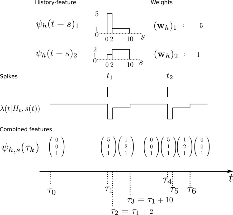
Figure 2. Illustration of the data-dependent time discretization. Two spikes from one neuron have been observed at time points t₁ and t₂. Since we assume a constant input (s(t) ≡ 1) the last entry in the combined feature vector ψ_h,s(t) is always 1. The spiking history up to time t, denoted with H_t is described with two basis functions, (ψ_h(t))₁, (ψ_h(t))₂. Each of these could have its own discretization, but here both have the same, namely at 0, 2 and 10 ms. That is, the basis functions are approximated with a piecewise constant function with jumps at 0, 2 and 10 ms. Each spiking history feature has its own weight, as has the stimulus. Thus, the feature vector describing both, the stimulus as well as the spiking history ψ_s,h(t) is a three-dimensional vector, changing its value at discretization-points τ_k. In each interval [τ_k,τ_k+1) the rate λ(τ_k | H_t, s(τ_k)) can be calculated. In this specific case, it only assumes three different values, exp(ψ_s,h(t)^Tw_h,s) = exp( − 27), exp( − 2), exp(1), assuming that the weight for the stimulus is w_s = 1.

Using Laplace Priors for Better Regularization

The expansion of the stimulus and the spiking history in high-dimensional feature spaces comes at the cost of having a large number of parameters to deal with. As we only have access to a limited amount of data, regularization is necessary to avoid overfitting. In the Bayesian framework, this can be done by choosing a prior distribution p(w) = p((w_s, w_h)) over the linear weights w_s and w_h. As these parameters enter the log-likelihood linearly, the prior distribution can be interpreted as specifying how likely we think that a particular feature is active, or necessary for explaining a typical data set. The prior distribution becomes more important as we increase the number of parameters.

Two commonly used priors are the Gaussian,

and the Laplace prior,

Given a prior distribution, one can write down the posterior distribution,

which specifies how likely a set of weights w is, given the observed data D and the prior belief over the weights. The data D contains both, observed spike trains as well as stimuli.

To obtain a particular choice of parameter values a popular point estimate is MAP estimate, that is the point of maximal posterior density argmax_w p(w | D). The MAP estimate is equivalent to the maximum likelihood estimate regularized with the log-prior. As mentioned above, the use of Laplace priors can yield advantageous regularization properties (Tibshirani, 1996 ; Lewicki and Olshausen, 1999 ; Ng, 2004 ; Steinke et al., 2007 ; Mineault et al., 2009 ). For a sparse prior, most of the features are likely to have zero weight, but if they have a non-zero weight, the amplitude is less constrained. In order to favor sparse solutions, the direct approach would be to penalize the number of non-zero parameter entries. The number of non-zero entries is sometimes referred to as the “L0-norm” of the parameter vector (despite the fact that it is not a proper norm). Unfortunately, finding the L0-norm regularized weights is a hard problem. Using the L1-norm however, is a useful relaxation which in some cases even gives an equivalent solution (Donoho and Stodden, 2006 ). The log of the Laplace prior-probability (see Eq. 10) of a given parameter vector is proportional to the L1-norm of this vector. Therefore, using a Laplace prior is equivalent to penalizing the L1-norm of the parameters. Finally using a Gaussian prior is equivalent to penalizing the L2-norm of the parameter vector (see Eq. 9).

From a practical point of view, log-concavity is another desirable property of the prior distribution as it here ensures that the posterior p(w|D) ∝ p(w)p(D|w) is also log-concave and therefore finding the maximum of the posterior (i.e., computing the MAP estimator) is a convex optimization problem (Paninski et al., 2004 ). For the GLM, log-concavity and convexity of the link function f is also required to guarantee log-concavity of the posterior. Both priors, the Gaussian as well as the Laplacian are log-concave. Although the posterior is log-concave when a Laplace prior is used, calculating the MAP is still a non-trivial problem. As the Laplace prior is non-differentiable at zero, the gradient at any point containing a zero in at least one component cannot be calculated. Thus standard techniques like conjugate gradient or iterative reweighted least squares fail. For the case of a Gaussian likelihood and Laplace prior the LASSO algorithm (Tibshirani, 1996 ) can be used. For the case of a likelihood originating from a GLM, the posterior is differentiable in each orthant, and hence subgradients can be calculated. In our implementation, we use the algorithm of Andrew and Gao (2007) .

Performance Measures

After we have obtained an estimate of the parameters of a GLM, we would like to evaluate the quality of the estimate.

Prediction performance

To measure the performance of an estimate, we calculated the difference between the estimated model and the ground truth model with respect to the log-likelihoods on a test set. The test set was generated with the same weights for each trial. In this way we can assess how likely a previously unseen spike train sampled from the ground truth model is under the estimated model. The difference between the average log-likelihoods can be seen as an approximation to the Kullback–Leibler distance of the estimated model from ground truth.

Here D_i is a spike train in the i-th of N trials generated with the true weights w whereas the estimated weights are The more likely the spike trains are, the better is the weight estimate, which specifies the estimated model. Therefore, the difference in log-likelihood of the different models measures how well the estimated model does at predicting spike times from the ground truth model.

Mean squared error reconstruction

A different way of quantifying the performance of an estimation algorithm for synthetic data would be to check how closely the estimated parameters match those that were put into the model as ground truth (w). In particular for judging the quality of the reconstructed filter shapes a popular choice is to look at the mean square error between the true and estimated parameters:

Approximating the Posterior Distribution Using EP

It has been shown that the MAP yield a good prediction performance (Pillow et al., 2008 ) but there are a couple of reasons why one would like to know more about the posterior than just its maximum. For example the posterior mean is known to be the optimal point estimate with respect to the mean squared error (Eq. 12). Furthermore, in many cases we are not only interested in a point estimate of the parameters, but we also want to know the dispersion of the posterior. In other words, we want to have confidence intervals indicating how strongly the parameters of a model are constrained by the observed data.

The resulting uncertainty estimate in turn can be used for optimal design (Lewi et al., 2008 ; Seeger, 2008 ), that is we can decide which stimulus to present next, in order to maximally reduce our uncertainty about the parameters. Furthermore, a distribution of the full posterior distribution gives rise to the marginal likelihood, which is the likelihood of the data under the model, without assuming specific linear filters. The marginal likelihood can be used to optimize the parameters of the prior without performing a crossvalidation (Chib, 1995 ; Seeger, 2008 ). Mathematically, the uncertainty is encoded in the dispersion of the posterior distribution over parameters w given observed data D :

where

Taken together there are strong arguments why it is useful to investigate the information conveyed by the posterior other than just the location of its maximum. The posterior is really the summary of all we can learn from the data about the given model.

Unfortunately, exact Bayesian inference (calculation of the normalization constant Z) is intractable in our case. Therefore, we are interested in finding a good approximation to the full posterior. If we can determine the posterior mean and covariance, this naturally leads to a Gaussian approximation of the posterior. Furthermore, we note that the true posterior in our case is unimodal, as both likelihood and prior are log-concave (Paninski, 2004 ). We employ the Expectation Propagation (EP) algorithm in order to compute a Gaussian approximation to the full posterior (Opper and Winther, 2000 , 2005 ; Minka, 2001 ; Seeger, 2005 ) (see Nickisch and Rasmussen, 2008 for alternative approximations schemes). The key observation is that the likelihood as well as the Laplace prior factorizes over simple terms, each of which is intrinsically one-dimensional. We have three types of factors:

where, u_i : = ψ_s,h(τ_i)^Tw_s,h defines the one-dimensional direction for each of these factors. ψ_s,h and w_s,h denote the concatenation of the feature vectors describing the spiking history and the stimulus history respectively. Equation 14 corresponds to a factor or individual term in the sum of the log-likelihood (Chichilnisky, 2001 ) if there was a spike at τ_i+1 and no spike in the interval (τ_i, τ_i+1) of length Δτ_i : = (τ_i+1 − τ_i). Equation 15 corresponds to a factor if there was no spike at time τ_i+1. Finally, Eq. 16 represents the Laplace terms for the prior in the product for the posterior distribution. The Expectation Propagation algorithm approximates each of those factors with a Gaussian factor:

Thus, if we multiply all of these approximating factors, we obtain a Gaussian distribution, which is straightforward to normalize:

with

The task now is to update the parameters π_i, b_i for the approximating factors such that the moments of the resulting approximation are as close to the true moments as possible. The crucial consistency equation which the EP algorithm tries to attain is given by Opper and Winther (2005) :

where D_KL denotes the Kullback–Leibler divergence or relative entropy. Q(u_i) is the marginal Gaussian distribution in the direction of ψ_s,h(τ_i). It is the Gaussian distribution one obtains, when taking the complete approximation Q(w) and projects it on ψ_s,h(τ_i). In other words, we require the approximation to be consistent in the sense that, if we replace the approximating factor with the true factor f_i(u_i), the marginal moments in the direction of ψ_s,h(τ_i) should not change. To achieve this consistency, EP cycles through the factors and updates the parameters of each approximating factor such that Eq. 23 holds. For Eq. 23 to hold, only moments of a one-dimensional distributions have to be calculated. This can efficiently be done using numerical integration (Piessens et al., 1983 ). We omit the details of this updating scheme here and refer to the Appendix. The interested reader is referred to our MATLAb code and to further literature (Heskes et al., 2002 ; Qi et al., 2004 ; Seeger et al., 2007 ). The computational cost of EP is quadratic in the number of parameters (as the posterior covariance has to be estimated) and linear in the number of factors (in the GLM setting this is the same as the number of discretization-points) per cycle through the factors. In our simulations 30 iterations through all factors were sufficient for convergence.

Another frequently used way of approximating the posterior distribution with a Gaussian, is the so called Laplace approximation or Laplace’s method (MacKay, 2003 ; Rasmussen and Williams, 2006 ; Lewi et al., 2008 ). A second-order Taylor expansion is calculated around the MAP. As the posterior is unimodal, the MAP can be found efficiently. Calculating the Hessian at a particular point can also be obtained analytically, given the posterior is differentiable at that point. The Laplace prior we use, however, is non-differentiable at zero. Therefore, the posterior is not differentiable at any point which contains at least one zero in one component. As we expect the MAP to assign many components zero weight, we cannot calculate the Hessian at that point. Furthermore, in a different setting it has been shown that the quality of the Laplace approximation is inferior to the one achieved by the EP approximation (Kuss and Rasmussen, 2005 ; Koyama and Paninski, 2009 ). The Laplace approximation is only sensitive to the local curvature at the point of maximal posterior density. As the EP approximation is based on moment matching it is influenced by the shape of the full posterior distribution.

Potential Uses and Limitations

In the following, we systematically compare the different point estimates, posterior mean and MAP. We vary the assumed prior distribution as well as the loss function in terms of which the performance is measured. In particular, we also investigate cases in which the assumed prior distribution differs from the “true” distribution used to generate the parameters. Finally, we also look at the possible effects of data discretization.

MAP Versus Posterior Mean

Tibshirani (1996) showed that for Gaussian likelihood and Laplace priors, the MAP gives sparse solutions and performs best, given the true underlying weights are sparse. If the data is assumed to be distributed according to a logistic likelihood, a similar result has been found by Ng (2004) . Here, for the case of data generated by a GLM, we would like to see whether the same holds true, and also compare the MAP to the posterior mean.

To illustrate the effect of a Laplace prior when increasing the number of features in the GLM of spiking neurons, we considered the following examples. We made a series of simulations with GLM neurons for which the space of possible features was successively increased from 10 to 230 dimensions. The stimulus was Gaussian white noise discretized into 10 ms bins. The stimulus history s(t) was set to contain the stimulus values of the last 20 bins describing the stimulus history for a period of 200 ms. From the 20 dimensional stimulus history s(t) we constructed the full 230 dimensional quadratic feature space:

with Δ = 10 ms, similar as in Rust et al. (2005) . From this basis of the 230 dimensional feature space a subset of increasing size was selected. That is, the dimensionality of the weight vector increased from 10 to 230, too. For all simulations, a GLM neuron was simulated until the likelihood consisted of 400 factors, i.e., 400 τ_k in the sum in Eq. 8 (alternatively one could also fix the time-duration of a trial or the number of spikes per trial).

We compared three different choices of priors, and use models which either had matching priors, or different ones:

1. Gaussian weights: Each weight was sampled independently from a Gaussian distribution. The variance was set to 20/dim(ψ_s).

2. Laplacian weights: Each weight was sampled independently from a Laplace distribution. The variance was set to 20/dim(ψ_s).

3. Sparse weights: A subset of only 10 dimensions was assigned with non-zero weights. For the assignment of the 10 weights, we draw 10 samples from a Laplace distribution with variance 2 and zero mean.

In Figure 3 the Kullback–Leibler distance is plotted as a function of the dimensionality of the feature space for each of the generating distributions. In Figure 3 A the weights of the ground truth model are sampled from a Gaussian distribution. Analogously, Figure 3 B shows the results for the Laplace distribution and Figure 3 C for the strongly sparse weights. We plot the average KL-divergence over 5000 trials ± 1 SD. As can be seen, the EP estimate for the Laplace (L1) prior performs best, if the true underlying weights are sparse. If the weights are sampled from a Laplace or a Gaussian distributions, the parameter vector of the true model is non-sparse and the L2 regularized MAP performs best. Interestingly, even for the case in which the weights are sampled from a Laplace distribution, the MAP performs best when using an L2-penalty term. Since we know the prior variance that was used to generate the weights, we did not perform a crossvalidation to set the regularization parameter, neither for the MAP estimates, nor for the posterior mean estimates (EPL1, EPL2). (Note that, in cases where the true distribution of weights is different to the prior used, it is possible that the prediction performance could be increased by picking a variance which is different to the “true” one).

FIGURE 3

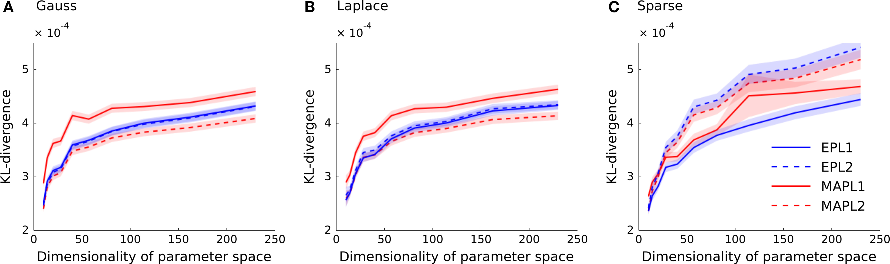
Figure 3. Prediction performance in high-dimensional feature spaces of increasing size. The mean across 5000 trials of the differences in the log-likelihoods is plotted as a function of increasing stimulus dimension. The different point estimates are MAP with Laplace regularization (MAPL1, solid red), MAP with a Gaussian prior (MAPL2, dashed red) and the posterior mean approximated with EP for the Laplace (solid blue) as well as for the Gaussian prior (dashed blue). Confidence intervals indicate standard error of the mean difference. Panel (A) shows the performance when a Gaussian distribution is used for sampling the weights and (B) for a Laplace distribution. (C) Shows the prediction performance if the weights are actually sparse, that is the true dimensionality is constantly 10. The overall variance for the generation of weights in panels (A) and (B) were kept fix to the same value as in (C).

In cases, in which the parameters are really drawn from the prior distribution, the posterior mean estimate can be shown to be the optimal parameter estimate, as it will minimize the mean squared error. Thus, in the two cases, in which we sampled the weights according to a Gaussian and a Laplacian distribution respectively, we expect the EP approximation to be superior to the MAP estimate in terms of the mean squared error. In the situation where the weights are actually sparse the performance is less clear, as the EP estimates assume a prior which is different to the one used to generate the weights. Therefore, it is not guaranteed in this case, that the posterior mean will be the optimal parameter estimate with respect to the mean squared error.

In general, we expect the MAP estimate to give a sparser solution than the posterior mean. If we have not seen much data, we expect the prior to dominate the posterior. In this case the maximum of the posterior will be at zero, resulting in a zero weight for the MAP. However, as the likelihood factors are not symmetric, the posterior is also not symmetric in general. Thus, even for weights for which the MAP is at zero, the probability mass is not symmetrically distributed around that maximum. Hence, the posterior mean in this case will be non-zero and the solution less sparse. In Figure 4 we plotted the mean squared reconstruction error for the different estimators. As can be seen the EP approximation to the posterior mean performs better than the MAP. This is also true for the sparse setting, however the effect gets less prominent if the dimensionality of the parameter space is increased.

FIGURE 4

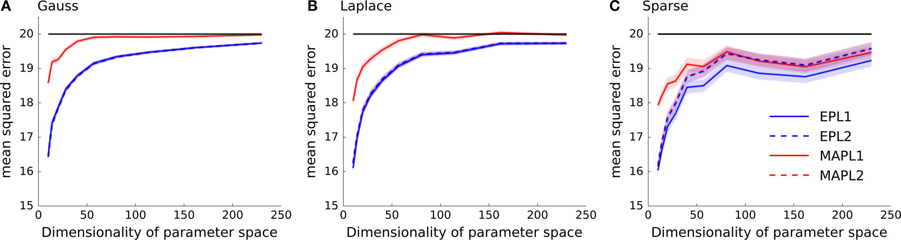
Figure 4. Mean squared error as a function of increasing dimensionality of the parameter space. The same data as in Figure 3 is plotted, but instead the performance is measured in mean squared error between the estimated weights and the true underlying weights as opposed to the differences in log-likelihoods shown in Figure 3 . (A) Shows the performance if the underlying weights are sparse, in panel (B) a Laplace distribution is used to sample the weights and in (C) a Gaussian distribution is used. In each panel the mean across 5000 trials is plotted ± standard error of mean. In solid black the prior variance is plotted, which is the expected mean squared error of the constant estimator.

The quality of the different point estimates, quantified by the mean squared error and by the prediction performance are summarized in Table 1 . To obtain a single number for the overall performance, we summed the errors for each individual dimension of parameter space (integral over each curve in Figures 3 and 4 ). The posterior mean gives a good estimate in all settings when a Laplacian prior is used. For the prediction performance the MAP with the L2 prior can lead to better results if the true prior is Gaussian or Laplacian.

TABLE 1

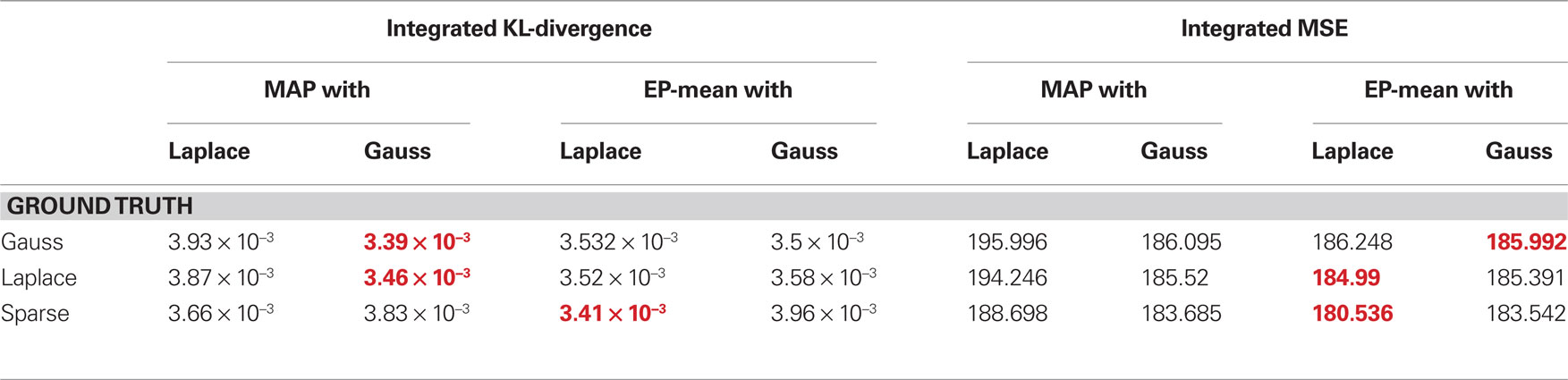
Table 1. Comparison of different quality measures and point estimates. In the left table integrated KL-divergence is shown for the MAP and the posterior mean point estimates when either a Laplace or a Gaussian prior is assumed. Each row corresponds to a ground truth prior which was used to sample the weights. Each number corresponds to an integral of a curve in Figure 3 . The right table reports the same when the mean squared error is used as a loss function. Thus, each number is the integral over one curve in Figure 4 and therefore reports the overall performance of the different estimators. For each ground truth model and loss function the best overall estimator is colored in red.

Binning and Identifiability

In Section “Generalized Linear Modeling for Spiking Neurons” we specified the log-likelihood in terms of time-discretized features. This results in a binning with not necessarily equidistant discretization-points τ_j. Another popular way to simplify the log-likelihood is to bin the time axis directly. In this section we would like to illustrate the possible effects of the two discretizations by means of a simple example. For some areas, for example in the auditory cortex, the precise timing of spikes is important (Carr and Konishi, 1990 ; Wightman and Kistler, 1992 ). By binning spikes into a discrete set of bins, one might lose this precise timing. If one discretizes the time axis directly and wants to keep the precise timing, one needs to specify very small time bins. This leads to a large number of discretization-points and hence very many factors for the likelihood. Alternatively, if one discretizes the features, the discretization is adapted to the spike times and thus could lead to possibly fewer discretization-points while still achieving a high temporal resolution. However, if a lot of spike times have been observed, discretization of the basis functions for the features could lead to a time discretization which is too fine for optimization purposes. A compromise would be to adaptively add discretization-points when needed, but constrain the minimal inter discretization-point interval. In general, the discretization of the features allows one to specify the resolution and (given that resolution) produces then the minimal number of discretization-points.

To illustrate possible differences between a discretization of features versus a discretization of the time axis, we considered the following example: two GLM neurons were simulated. One of them had a stimulus filter, while the other one was only dependent on the spikes from the first neuron. The filters for the stimulus as well as the spiking history filters are illustrated in Figure 5 (black lines). Because the second neuron was positively coupled to the first one with a small latency, we expect it to produce spikes which have a small temporal offset with respect to the spikes of the first neuron. Intuitively, the observed spikes trains could be explained by two different settings:

FIGURE 5

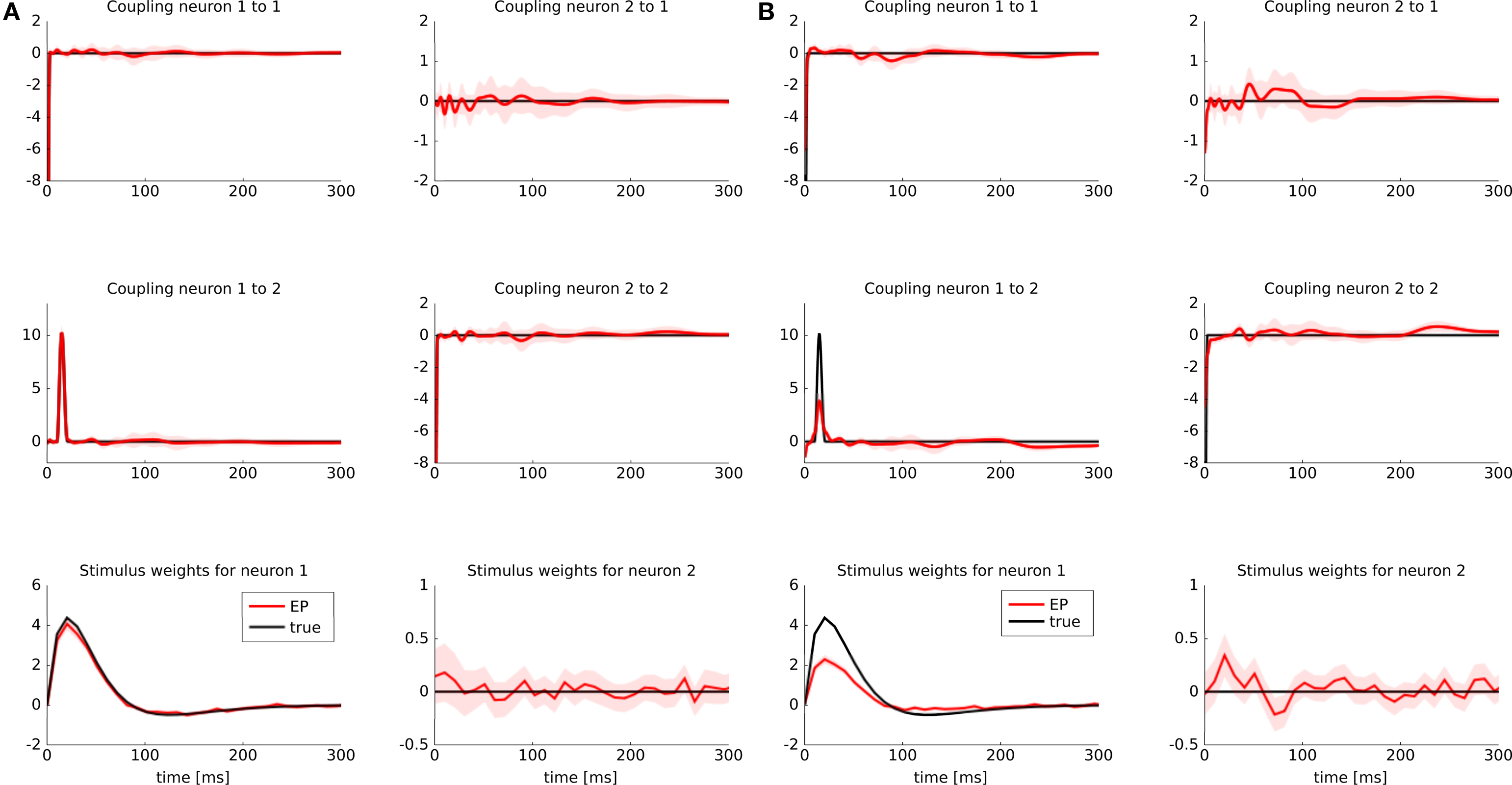
Figure 5. Identifyability in the presence of binning noise. (A) Estimated filters, when the features are discretized (approximated with a piecewise constant function, see Figure 2 ). (B) Estimated filters when the spike times are binned. The binning was performed such that at most one spike fell into one bin. All spikes were aligned to the right hand side of their corresponding bins. When the time axis is binned directly and hence the precise timing of a spike is lost, the estimated filter for the spiking history are slightly weaker than the true ones (black), whereas the stimulus filters are slightly positive at a small latency. For the sake of readability we only plotted the approximated posterior mean (±2σ).

1. The weights are exactly as the ones used for simulating the spike trains.

2. The second neuron is not coupled to the first neuron at all, but has the same stimulus filter as the first one, however, with a small latency. Therefore it responds to the same stimulus but at later times.

If spikes were generated deterministically, these two setting cannot be distinguished. In the noisy case, however, given a sufficient amount of data, one should be able to disentangle the two scenarios, as finding the maximum likelihood point is a convex problem. However, for finite amount of training data and in the presence of binning noise, the situation is less clear. Therefore, we sampled 3 s of spike trains and estimated the parameters from the data, once when the features are discretized and once when the time axis is discretized. The time bins were chosen such that at most one spike fell into a bin.

The estimate for the approximated posterior mean are plotted in Figure 5 . If the features are discretized the filter could be recovered. If we discretize the time directly, we see indeed a slight shift toward the second scenario. That is, the stimulus filter for the second neuron in that case is slightly elevated, whereas the strength of the coupling filter is diminished.

Population of Retinal Ganglion Cells

To compare the different methods for the analysis of real data, we applied the algorithms to multi-electrode recordings of seven salamander retinal ganglion cells. Our goal was to describe the stimulus selectivity of the population by fitting a GLM with history terms and cross-neuron terms to the recorded data. We used multi-electrode recordings of salamander retinal ganglion cells generously provided by Michael J Berry II. The dataset has been published in Fairhall et al. (2006) , where all recording details are described. We selected a recording of seven neurons, which had an average firing rate of 1.1 spikes per second and a minimal interspike-interval of 2.8 ms. The stimulus used in the experiments consisted of 20 min white noise full-field flicker with a refresh rate of 180 Hz. To illustrate the ability of the model to also infer population models from small data sets, we fitted the population recording to the first 2 min of the recording.

For the features describing the spiking history, we used the density function of the Γ-distribution with different parameters as basis functions:

where the means α_i/β_i as well as the variances were logarithmically spaced between 1 and 700 ms and 1 and 1000 respectively (A similar basis consisting of raised cosines was also used in Pillow et al. (2005 , 2008) . Due to the logarithmic spacing, we have a finer resolution for small time-lags and coarser resolution for long time-lags. For example, we expect the first basis function, which has a sharp peak at zero to be mainly active or associated with the refractory period. As we discretize the basis functions rather than directly the time axis, each spike generates as many discretization-points τ_j as there are discretization-points for the basis functions (see Section “Generalized Linear Modeling for Spiking Neurons”). For the stimulus we used the same basis function set. As for the spike history dependence these functions were approximated with a piecewise constant function. The discretization for the basis-function time axis in this case was the same as for the original stimulus and therefore slightly coarser than the one for the spike history features. The basis functions are plotted in Figure 6 .

FIGURE 6

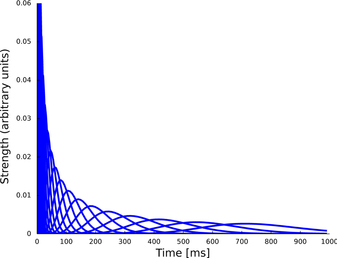
Figure 6. Set of 23 basis functions to span the spiking history as well as the stimulus dependence. Each function is a density function of a Γ-distribution with different means and variances, see Eq. 24. The time axis for the features describing the spiking history was logarithmically discretized up to 1000 ms.

For this setup we computed the different point estimates and posterior approximations for the weights corresponding to the features describing the spike history dependence (Figure 7 ) as well as for the weights corresponding to the stimulus filters (Figure 8 ).

FIGURE 7

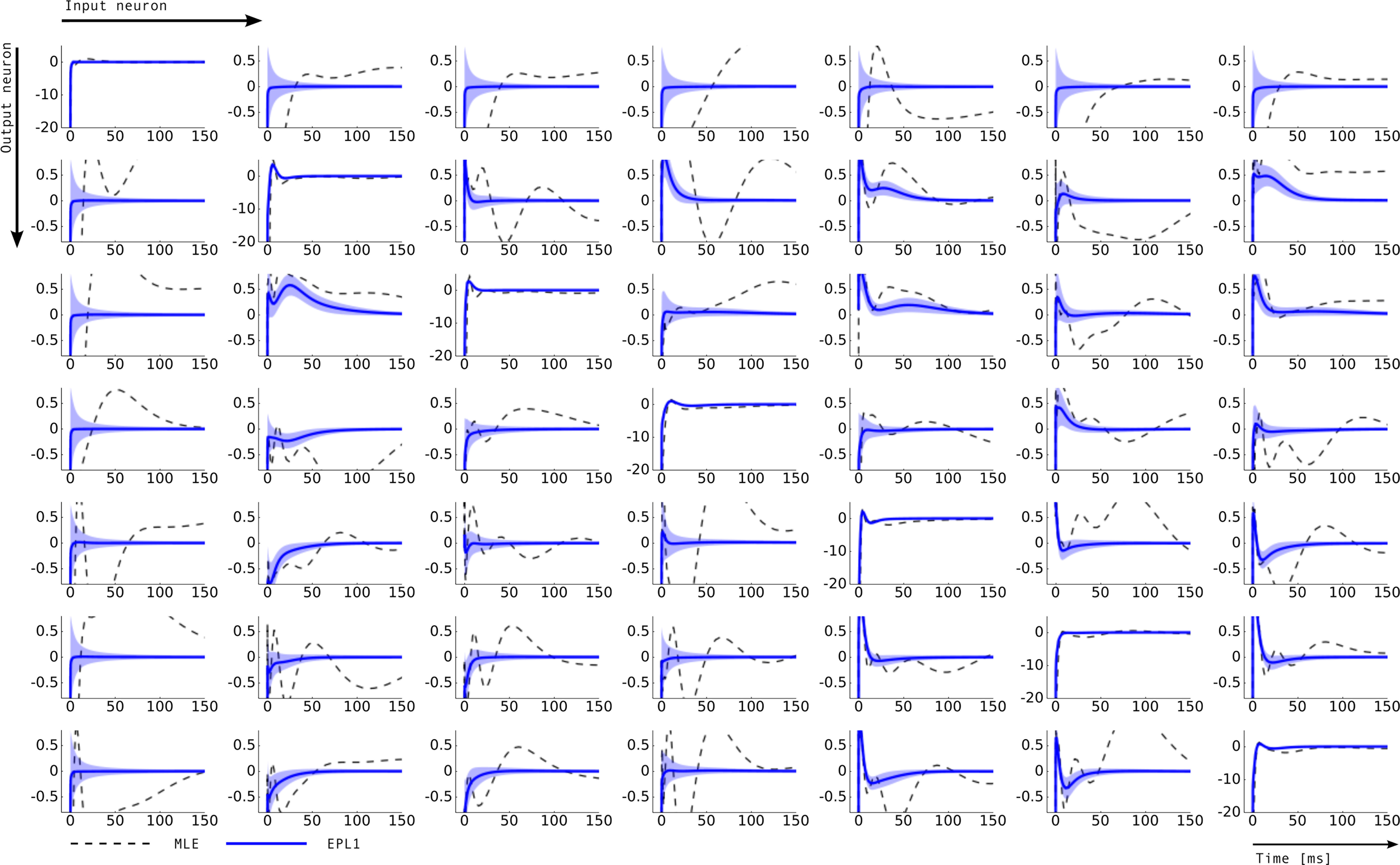
Figure 7. Inferred connectivity in the network of seven retinal ganglion cells. Plotted are the induced dependencies by the weights, that is the superposition of basis functions, weighted by the inferred weights from two different estimators: maximum likelihood (MLE) and approximated posterior when a Laplace prior is used (EPL1). For the EP approximation the posterior mean together with 2 SD is plotted. Each row corresponds to one output neuron and each column corresponds to a input neuron. Thus, the entry (i, j) describes the influence of a spike of neuron j on the firing rate of neuron i. For example on the diagonal a strong negative coupling on a short time-scale can be observed, representing the refractory period of a neuron. The maximum likelihood estimate as well as thee posterior mean agree on the self-feedback but exhibit a large difference on some couplings, e.g., neuron 1 → 4. In general, neuron 1 seems to be less constrained than other neurons, which is also indicated by the large uncertainty intervals for the connections from and to neuron 1.

FIGURE 8

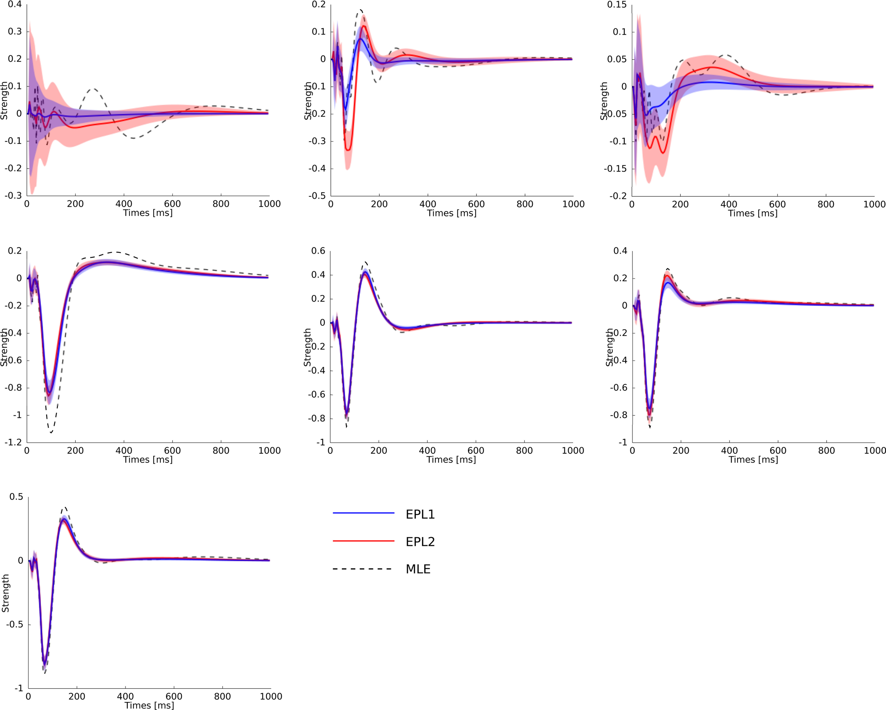
Figure 8. Statistical dependence of the neural activity of seven neurons on the stimulus specified by the superposition of the basis functions plotted in Figure 6 weighted by the estimated weights. The same colors for the different estimators as in Figure 7 are used. Additionally the posterior mean (±2σ confidence intervals) for the EP approximation with a Gaussian prior is plotted in red. Each plot corresponds to one neuron in the same order as in Figure 7 . As can be seen, the maximum likelihood estimator is overfitting. One sees, that the posterior uncertainty for neuron 1 and also for neuron 3 are much larger as for the other neurons analog to Figure 7 .

For training, only 2 min out of the 20 min of recording were used. Another 2 min were used for setting hyperparameters, i.e., prior variances. Given the posterior variances for each of the weights and the basis functions, we can calculate errorbars on the time course of the coupling and stimulus filters. The filters are defined as the weighted sum of the basis functions. For example, the gamma-functions f_i in Eq. 24 are weighted by the weights, corresponding to the entry in the feature vector ψ_h. Errorbars on the coupling filter f(t) can then be estimated using the marginal variances:

where f(t) is a vector of the corresponding basis functions f_i(t) and Cov[w|D] is part of the posterior covariance matrix corresponding to the weights for the features described by f_i(t). In the above equation D represents the dataset used for training, containing both, stimulus and spike trains. To illustrate this, we also plotted confidence regions of 2 SD for the coupling parameters of the population. The confidence intervals for the Gaussian approximation are plotted in red when a Laplacian prior is used and in gray when a Gaussian prior is used. Based on the confidence intervals for the coupling filters, only a few of the connections are actually significant, as can be seen in Figure 7 . This cannot be concluded from the couplings estimated via MAP or MLE. For example, we see that connections to neuron 1 (first column in Figure 7 ) as well as connections from neuron 1 to any other neuron (first row) are underconstrained by the data, indicated by the large uncertainty for those connections compared to those for others. Consequently, the connections are set to zero by the prior and hence effectively excluded from the model. The strong negative self-feedback coupling, indicating the refractory period can be estimated with a much higher degree of certainty. We also find some significant couplings between neurons, both negatively coupled (e.g., neuron 2 → 5) and positively coupled (e.g., 7 → 2). The maximum likelihood estimator assigns a non-zero filter to almost every coupling between neurons. The EP-mean, however, forces most of the filters to be zero. To quantify the difference in the estimated filters, we calculated the squared difference between the maximum likelihood and the EP-mean weights. This squared difference is 1.5 times larger than the average squared norm of the individual parameter vectors, which indicates that not only the absolute value of the maximum likelihood estimator is larger but also the qualitative shape is different. On the other hand the differences in prediction performance as measured by the likelihood is rather small (see Table 2 ). Thus, proximity in terms of one quality measure need not necessarily imply proximity in terms of the other as well. If the posterior uncertainty is small, the parameter vectors are much more constrained by the data and the filters estimated by the maximum likelihood estimator are closer w.r.t. the mean squared distance to the EP-mean. For example this is true for most of the stimulus filters (see Figure 8 ). In contrast, if the posterior uncertainty is rather large, for example for the stimulus filters of neuron 1 and neuron 3, the estimated weights differ more. This suggests, that we do not have sufficient information to estimate all parameters, but we are able to extract some weights from the given data.

TABLE 2

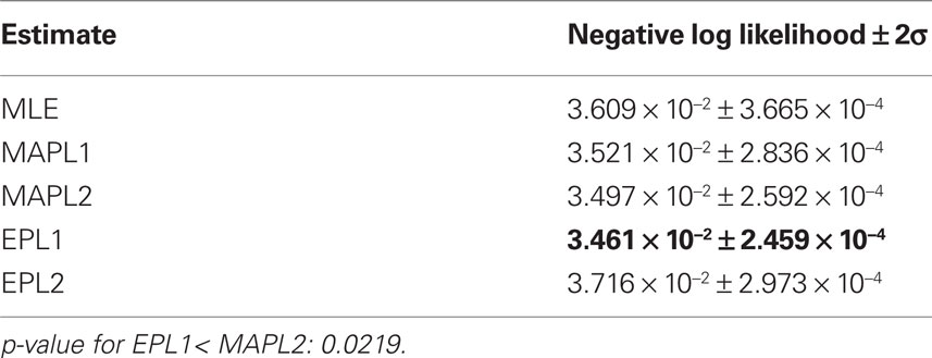
Table 2. Mean prediction performance of different point estimates averaged over 16 test sets of 1 min length. As we do not have access to the true underlying model, the prediction performance here is measured in negative log-likelihood score not in differences in likelihoods.

To compare the different estimators quantitatively, we used the same performance measure as for Figure 3 , namely the negative log-likelihood on a test set. To obtain confidence intervals on the performance measure we split the part of the dataset, neither used for training nor for validation into 16 different test sets (10%, i.e., 2 min for training, 10% for validation and 80% for testing, split into 16 sets of 1 min length). The performance values are summarized in Table 2 . By this performance measure the EP estimate with a Laplacian prior performs significantly better than the MAP estimate with the same prior. The performance difference to the maximum likelihood estimator is not huge, this indicates, that the weights are not sufficiently constrained by 1 min slices of the data. Especially the coupling terms not well constrained as can be seen by the difference in the estimated filter by the maximum likelihood and the posterior mean, see Figure 7 . By judging from the data, we do not know if the couplings are needed, hence excluding them from the model, i.e., setting the corresponding weights to zero, seems to be a safe choice. This can be achieved by using a strong prior distribution. The difference between a Gaussian and a Laplace prior is not large for the coupling terms (not shown), for the stimulus filters we see a small difference for the first three neurons, see Figure 8 . Note, that in cases where there is a significant coupling between neurons, the EP and the maximum likelihood fit agree.

Discussion

Bayesian inference methods are particularly useful for system identification tasks where a large number of parameters need to be estimated. By specifying a prior over the parameters a full probabilistic model is obtained that provides a principled framework for regularizing the model complexity. Furthermore, knowledge of the posterior distribution allows one both to derive point estimators that are optimized for loss functions that are suitable to the problem at hand and to quantify the uncertainty about such estimates.

A major hurdle for using a Bayesian approach is that computing the posterior distribution is often intractable. Even for numerical approximation techniques of the posterior distribution there is usually – a priori – no guarantee how well they work. Therefore, it is important to perform careful quality control studies if such methods are to be applied to a new estimation problem. In this paper, we presented such control studies for approximate Bayesian inference in the GLMs of spiking neurons using Expectation Propagation (EP) and compared it to standard methods like maximum likelihood and MAP estimates. Expectation Propagation provides both a posterior mean and a posterior covariance approximation. These first and second-order moments are sufficient to obtain a rough sketch of the location and dispersion of the posterior distribution. The posterior mean, in particular, can be used as a point estimator which is known to minimize the mean squared error loss. This loss function is an expedient choice if one aims at reconstructing the filter shapes. As we have shown in this work, the posterior mean estimate obtained with EP yields a smaller mean squared reconstruction error of the parameters than maximum likelihood or MAP estimation.

It should be noted, however, that the filter shapes represent statistical couplings only. Clearly, the existence of a statistical coupling does not necessarily imply the existence of a physical coupling as well. Statistical dependence could, for example, also be a consequence of common input, or other indirect couplings. In fact, it is known that noise correlations between retinal ganglion cells are mainly due to common input, and not direct synaptic couplings (Trong and Rieke, 2008 ). In the model an inferred coupling simply indicates that there is a dependence between the neurons which cannot be explained by the stimulus filters or the neural self-couplings.

Receptive field estimation aims at a functional characterization of neural response properties. Therefore, it is natural to compare different estimates by asking how well they can predict spike trains generated in response to new test data. Evaluating the performance of predicting a particular spike train is often based on the use of a spike train metric (Victor and Purpura, 1997 ), as the predicted spike trains have to be compared to the observed spike trains. In general, one wants to compare models, and not only particular spike trains, and therefore averages the prediction performance across very many samples from the two models one wants to compare.

The Bayesian framework offers a principled way to obtain an optimal point estimate which minimizes the loss function averaged across the posterior distribution. Although it is unlikely that this optimization problem can be solved analytically, one can sample weights from the posterior and then sample several spike trains for these given weights. In other words, we can generate samples from the predictive distribution. For the prediction performance measure specified by the loss in Eq. 11, for example, an optimal point estimate would be given by those weights which on average yield the largest likelihood for the ensemble of spike trains drawn from the predictive distribution. Neither the MAP nor the posterior mean is optimal with respect to this criterion. Theoretically, the MAP is optimized for the zero-one-loss, whereas the posterior mean is optimized for the squared error loss (Lehmann and Casella, 1998 ). In Appendix “Bayes-Optimal Point Estimate for Average Log-Loss”, we demonstrate on a simple, concrete example (estimation of the probability of a coin flip and log-loss as loss function) that an optimized predictor will perform better (on average) than the MAP estimate, irrespective of what data was observed. Clearly, this approach is only possible if one has at least an approximate model of the posterior, as we have presented here.

For a single GLM this will yield a set of parameters which are guaranteed to be optimal on average. The optimality of course only holds if the model is correct (i.e., the observed spike trains are indeed samples from a GLM), the prior is appropriately chosen, and the posterior distribution can be calculated precisely. In practice, it is not clear how justifiable each of the the three assumptions is going to be. Therefore, it is an interesting open question of how much better point estimates which are optimized using this approach will perform when compared to other optimization methods. Empirically, we observed that the posterior mean estimate obtained with EP is always better then the MAP with respect to squared error loss. With respect to the prediction error, the MAP performed slightly better than the EP posterior mean estimate if the weights were drawn from a Gaussian or Laplacian distribution, while the EP posterior mean was better than the MAP estimator if the weights were drawn from the truly sparse distribution. Of course, one could also directly use the predictive distribution as it will in general assign higher likelihood to unseen spikes than any point estimate. However, the predictive distribution cannot be described by a single GLM as it is an average over many models.

Our study also provides some insights about the effect of different kinds of prior distributions on the estimation performance. The choice of prior in the Bayesian framework offers a principled way of regularization. Here, we compared specifically a Gaussian and a Laplacian prior. While there was almost no difference in performance between the EP posterior mean estimator for the Laplacian and the Gaussian prior if the true prior was Gaussian or Laplace, the assumption of a Laplacian prior led to a substantial advantage when the true weight vectors had only a few non-zero components. This confirms the intuition that one can profit from using a Laplacian prior if one sets up a large number of candidate features of which only a few are likely to be useful in the end. Interestingly, for the MAP estimator, the use of a Laplacian prior almost always led to a substantial impairment and resulted in a relatively small improvement only w.r.t. the prediction performance if the weights were sampled from a sparse distribution for which almost all coefficients are zero.

While the posterior mean, and even more so the MAP estimator can strongly depend on the particular choice of prior distribution, this indeterminacy is a problem only if the dispersion of the posterior distribution is not taken into account appropriately. This is a strong case for the use of EP as the MAP estimator does not provide any control to what extent the result is actually constrained by the data. By also computing the posterior covariance rather than just a point estimator, we obtain confidence intervals which can serve exactly to this purpose. For the retinal ganglion cell data analyzed in Section “Population of Retinal Ganglion Cells”, for example, it allowed us to distinguish between neuronal couplings, that are significant and others which were not (see neuron 1 in Figure 7 ). One can also see that whenever the confidence intervals were large, the maximum likelihood estimator deviated substantially from the Bayesian point estimators.

Appendix

Expectation Propagation with Gaussians

Finding the posterior moments

In the following we will explain the essentials for approximating posterior distributions with a Gaussian distribution via the Expectation Propagation algorithm.

Suppose the joint distribution of a parameter vector of interest w and n independent observations D = {x₁,…,x_n} factors as:

where p(w) is a chosen prior distribution. Further we assume, that each of the likelihood factors depends on a linear projection of the parameters w only. That is, a likelihood factor can be written as:

Hence, each likelihood factor is intrinsically one-dimensional. Next, we choose an (un-normalized) Gaussian with which we would like to approximate each of those factors:

Plugging this into Eq. A1, we obtain for the approximation Q(w|D) to the posterior:

The prior distribution p(w) is allowed to have two different forms. It can either be a Gaussian in which case the inverse prior covariance has to be added to the outer products of the features ψ_i. Another option is, that the prior distribution also factorizes into intrinsic one-dimensional terms. This would be the case for example, if a Laplace prior is used.

with

In order to obtain the desired Gaussian approximation to the true posterior, the problem is now to find the parameters π_i, b_i. Once these parameters are found, we get the desired approximation via Eq. A1. If the posterior consists of a single factor, then the desired parameters π₁, b₁ are easily obtained via moment matching. The moments usually have to be calculated by a numerical one-dimensional integration along the direction ψ₁. To incorporate a new factor, we fix the parameters of the first one and try to find suitable b₂,π₂ for the second factor. More precisely, we want to minimize the Kullback–Leibler distance:

As both Q distributions are the same and all other factors vary only along one dimension ψ₂, the only degree of freedom we have are the moments in that direction (see Seeger, 2005 ). Technical speaking, we can split the integration of the Kullback–Leibler distance into two parts. One over the direction ψ₂ and one in the orthogonal direction. Now, for notational simplicity, we denote The moments of the Gaussian side in Eq. A8 can easily be computed by looking at the exponent. Let μ₁, σ₁ be the moments of the Q distribution in the direction of ψ₂:

Now, these moments have to be matched with the numerically obtained ones of Q(u₂|{x₁}) p(x₂|u₂) by adjusting π₂, b₂. This can be done, by choosing the parameters according to:

In this fashion we can incorporate one likelihood factor after another. This procedure is known as assumed density filtering (see Minka, 2001 ). The obtained approximation to the posterior depends on the order in which we incorporate the likelihood factors. The idea of Expectation Propagation is not to stop after one such sweep over the factors. EP rather tries to fulfill the consistency (Opper and Winther, 2005 ):

That is, we replace one of the approximating factors with the original one and require the moments not to change. To achieve this, one usually select an arbitrary factor i and divide it out of the current approximation. The resulting distribution is called the cavity distribution Q^\i(w). If we call the current moments of the approximation μ, Σ, the moments in the direction of ψ_i are given by:

Thus, we have for the cavity distribution:

Where we have abbreviated By using the same algebra as before, we have for the moments of the cavity distribution:

Now, we are in the same situation as before, because we want to update the parameters π_i, b_i in order to match the moments of the approximation to the ones of the cavity distribution times the original factor. These moments have to be calculated numerically, which can efficiently be computed as the involved integrals are only one-dimensional. We call these numerical moments

The moments have to match those of the complete approximation which gives:

Now we can plug in the definition of the moments of the cavity distribution to get an update for the parameters:

Together with Eq. A5 this results in a rank one update of the full distribution over the complete parameter vector w. More precisely we have a rank one update of the covariance matrix of the approximating Gaussian as well as an update of the mean:

Where we have used the Woodbury identity to obtain Eq. A30. To implement these equations in a numerically stable manner, one usually represents the covariance by it Cholesky decomposition:

where L is a lower triangular matrix. To calculate the moments for the Laplace factors, we used a technique by Seeger (2008) as numerical integration of Laplace factors can unstable.

Marginal likelihood

The marginal Likelihood for the hyperparameters θ is defined by:

When considering only the parameters π_i, b_i, EP gives us an un-normalized approximation to the likelihood factors As long as one is interested in the posterior only, this does not matter, because:

However, if we want to approximate the marginal likelihood we need the C_i explicitly:

The idea is to not only match the moments but the 0th moments as well. We require the expectation of P(x_i | w) and under Q^\i(w) to be the same for all i, from which we obtain:

For the we have:

Therefore, we have for the marginal likelihood:

One can also calculate gradients of the marginal likelihood with respect to hyperparameters (see Seeger, 2005 ).

MATLAB toolbox

Along with the paper we publish a MATLAB toolbox for inference in a generalized linear models http://www.kyb.tuebingen.mpg.de/bethge/code/glmtoolbox/ . The code provides routines for:

1. Sampling spike trains from a GLM

2. Calculation of different point estimators: maximum likelihood, MAP, posterior mean

3. Approximation of the posterior covariance via EP.

Either a Laplacian or a Gaussian prior can be specified. For the Gaussian prior an arbitrary covariance matrix is allowed.

Bayes-Optimal Point Estimate for Average Log-Loss

In the following we consider a simple example of a coin flip to illustrate the potential benefit of an optimized point estimate for the expected loss after having observed the data. Let x be Bernoulli distributed with unkown parameter θ ∈ [0, 1]. If we observe N data points x_i ∈ {0, 1} with k ones and assume a uniform prior over θ ∼ U[0, 1], we can compute the posterior distribution for θ:

which is a Beta-distribution with parameters α = k + 1, β = N + 1. The posterior mean is given by μ = (k + 1)/(N + 2). We define the average log-loss to be:

Then, we can calculate the expected average log-loss after having observed the data {x_i}:

F can now be minimized with respect to the point estimate The derivative with respect to is given by:

Therefore the posterior mean optimizes the expected prediction performance as measured by the average log-loss. We can also calculate the difference in expected performance between the posterior mean and the MAP, which is given by θ_MAP = k/N. The difference in expected performance is given by:

The difference in expected log-loss is the Kullback–Leibler divergence between the distribution corresponding to the optimized estimate (the posterior mean) and the distribution induced by the MAP estimate. As the Kullback–Leibler divergence is always non-negative, this shows that the loss incurred by the MAP estimate is greater than the optimized estimate, irrespective of the data (k) that was observed. In the extreme cases, i.e., k = 0 or k = N, the difference becomes infinite. This simple example shows that, in principle, an extra gain in performance can be achieved by optimizing the parameters for the expected performance over the posterior distribution.

Conflict of Interest Statement

The authors declare that the research was conducted in the absence of any commercial or financial relationships that could be construed as a potential conflict of interest.

Acknowledgments

This research was funded by the German Ministry of Education, Science, Research and Technology through the Bernstein award to Matthias Bethge (BMBF, FKZ:01GQ0601), and the Max Planck Society. We would like to thank Michael Berry for generously providing us with multi-electrode recording data to illustrate the method. Additionally, we thank Fabian Sinz and Philipp Berens for discussions and comments on the manuscript. A brief version of portions of this research were previously published as “Bayesian Inference for Spiking Neuron Models with a Sparsity Prior” in the proceedings “Advances in Neural Information Processing Systems 20 (2008)” (Gerwinn et al., 2008 ).

References

Andrew, G., and Gao, J. (2007). “Scalable training of L1-regularized log-linear models,” in ICML ‘07: Proceedings of the 24th International Conference on Machine Learning, Corvalis, OR (New York, NY: ACM), 33–40.

Borisyuk, G. N., Borisyuk, R. M., Kirillov, A. B., Kovalenko, E. I., and Kryukov, V. I. (1985). A new statistical method for identifying interconnections between neuronal network elements. Biol. Cybern. 52, 301–306.

Pubmed Abstract | Pubmed Full Text | CrossRef Full Text

Brillinger, D. R. (1988). Maximum likelihood analysis of spike trains of interacting nerve cells. Biol. Cybern. 59, 189–200.

Pubmed Abstract | Pubmed Full Text | CrossRef Full Text

Carr, C. E., and Konishi, M. (1990). A circuit for detection of interaural time differences in the brain stem of the barn owl. J. Neurosci. 10, 3227–3246.

Pubmed Abstract | Pubmed Full Text

Chib, S. (1995). Marginal Likelihood from the Gibbs Output. J. Am. Stat. Assoc. 90, 1313–1321.

CrossRef Full Text

Chichilnisky, E. J. (2001). A simple white noise analysis of neuronal light responses. Network 12, 199–213.

Pubmed Abstract | Pubmed Full Text

Chornoboy, E. S., Schramm, L. P., and Karr, A. F. (1988). Maximum likelihood identification of neural point process systems. Biol. Cybern. 59, 265–275.

Pubmed Abstract | Pubmed Full Text | CrossRef Full Text

Daley, D. J., and Vere-Jones, D. (2008). An Introduction to the Theory of Point Processes. Vol. II: General Theory and Structure. New York: Springer.

Donoho, D. L., and Stodden, V. (2006). “Breakdown point of model selection when the number of variables exceeds the number of observations,” in Proceedings of the International Joint Conference on Neural Networks (Piscataway: IEEE), 16–21.

Fairhall, A. L., Burlingame, C. A., Narasimhan, R., Harris, R. A., Puchalla, J. L., and Berry, M. J. (2006). Selectivity for multiple stimulus features in retinal ganglion cells. J. Neurophysiol. 96, 2724–2738.

Pubmed Abstract | Pubmed Full Text | CrossRef Full Text

Gerwinn, S., Macke, J., Seeger, M., and Bethge, M. (2008). “Bayesian inference for spiking neuron models with a sparsity prior,” in Advances in Neural Information Processing Systems 20, eds J. C. Platt, D. Koller, Y. Singer and S. Roweis (Cambridge, MA: MIT Press), 529–536.

Harris, K. D., Csicsvari, J., Hirase, H., Dragoi, G., and Buzsáki, G. (2003). Organization of cell assemblies in the hippocampus. Nature 424, 552–556.

Pubmed Abstract | Pubmed Full Text | CrossRef Full Text

Heskes, T., Zoeter, O., Darwiche, A., and Friedman, N. (2002). “Expectation propagation for approximate inference,” in Proceedings UAI-2002, eds A. Darwiche and N. Friedman (San Francisco: Morgan Kaufmann), 216–233.

Koyama, S., and Paninski, L. (2009). Efficient computation of the maximum a posteriori path and parameter estimation in integrate-and-fire and more general state-space models. J. Comput. Neurosci. doi: 10.1007/s10827-009-0150-x

CrossRef Full Text

Kulkarni, J. E., and Paninski, L. (2007). Common-input models for multiple neural spike-train data. Network 18, 375–407.

Pubmed Abstract | Pubmed Full Text | CrossRef Full Text

Kuss, M., and Rasmussen, C. E. (2005). Assessing approximate inference for binary Gaussian process classification. J. Mach. Learn. Res. 6, 1679–1704.

Lehmann, E. L., and Casella, G. (1998). Theory of Point Estimation. New York: Springer Verlag.

Lewi, J., Butera, R., and Paninski, L. (2008). Sequential optimal design of neurophysiology experiments. Neural. Comput. 21, 619–687.

CrossRef Full Text

Lewicki, M. S., and Olshausen, B. A. (1999). Probabilistic framework for the adaptation and comparison of image codes. J. Opt. Soc. Am. 16, 1587–1601.

CrossRef Full Text

MacKay, D. J. C. (2003). Information Theory, Inference and Learning Algorithms. Cambridge: Cambridge University Press.

McCullagh, P., and Nelder, J. A. (1989). Generalized Linear Models. New York: Chapman and Hall/CRC.

Mineault, P. J., Barthelmé, S., and Pack, C. C. (2009). Improved classification images with sparse priors in a smooth basis. J. Vis. 9, 10–17.

CrossRef Full Text

Minka, T. P. (2001). A Family of Algorithms for Approximate Bayesian Inference. PhD thesis, Massachusetts Institute of Technology, Cambridge.

Ng, A. Y. (2004). “Feature selection, L1 vs. L2 regularization, and rotational invariance,” in Proceedings of the Twenty-first International Conference on Machine Learning (New York, NY: ACM), 78–85.

Nickisch, H., and Rasmussen, C. E. (2008). Approximations for binary gaussian process classification. J. Mach. Learn. Res. 9, 2035–2078.

Nykamp, D. Q. (2008). Pinpointing connectivity despite hidden nodes within stimulus-driven networks. Phys. Rev. E Stat. Nonlin. Soft Matter Phys. 78, 021902.

Pubmed Abstract | Pubmed Full Text | CrossRef Full Text

Okatan, M., Wilson, M. A., and Brown, E. N. (2005). Analyzing functional connectivity using a network likelihood model of ensemble neural spiking activity. Neural. Comput. 17, 1927–1961.

Pubmed Abstract | Pubmed Full Text | CrossRef Full Text

Opper, M., and Winther, O. (2000). Gaussian processes for classification: mean-field algorithms. Neural. Comput. 12, 2655–2684.

Pubmed Abstract | Pubmed Full Text | CrossRef Full Text

Opper, M., and Winther, O. (2005). Expectation consistent approximate inference. J. Mach. Learn. Res. 6, 2177–2204.

Paninski, L. (2004). Maximum likelihood estimation of cascade point-process neural encoding models. Network 15, 243–262.

Pubmed Abstract | Pubmed Full Text | CrossRef Full Text

Paninski, L., Pillow, J., and Simoncelli, E. P. (2004). Maximum likelihood estimation of a stochastic integrate-and-fire neural encoding model. Neural. Comput. 16, 2533–2561.

Pubmed Abstract | Pubmed Full Text | CrossRef Full Text

Piessens, R., de Doncker-Kapenga, E., Uberhuber, C. W., and Kahaner, D. K. (1983). QUADPACK: A Subroutine Package for Automatic Integration. Berlin: Springer.

Pillow, J. (2009). “Time-rescaling methods for the estimation and assessment of non-Poisson neural encoding models,” in Advances in Neural Information Processing Systems 22, eds Y. Bengio, D. Schuurmans, J. Lafferty, C. K. I. Williams and A. Culotta (Cambridge, MA: MIT Press), 1473–1481.

Pillow, J., Paninski, L., Uzzell, V. J., Simoncelli, E. P., and Chichilnisky, E. J. (2005). Prediction and decoding of retinal ganglion cell responses with a probabilistic spiking model. J. Neurosci. 25, 11003–11013.

Pubmed Abstract | Pubmed Full Text | CrossRef Full Text

Pillow, J., Shlens, J., Paninski, L., Sher, A., Litke, A. M., Chichilnisky, E. J., and Simoncelli, E. P. (2008). Spatio-temporal correlations and visual signalling in a complete neuronal population. Nature 454, 995–999.

Pubmed Abstract | Pubmed Full Text | CrossRef Full Text

Pillow, J., and Simoncelli, E. P. (2006). Dimensionality reduction in neural models: an information-theoretic generalization of spike-triggered average and covariance analysis. J. Vis. 6, 414–428.

Pubmed Abstract | Pubmed Full Text | CrossRef Full Text

Qi, Y. A., Minka, T. P., Picard, R. W., and Ghahramani, Z. (2004). “Predictive automatic relevance determination by expectation propagation,” in Proceedings of the Twenty-first International Conference on Machine Learning. New York, NY: ACM.

Rasmussen, C. E., and Williams, C. K. I. (2006). Gaussian Processes for Machine Learning. Cambridge, MA: MIT Press.

Rieke, F., Warland, D., van Steveninck, R. R., and Bialek, W. (1997). Spikes: Exploring the Neural Code. Cambridge, MA: MIT Press.

Rust, N. C., Schwartz, O., Movshon, J. A., and Simoncelli, E. P. (2005). Spatiotemporal elements of macaque v1 receptive fields. Neuron 46, 945–956.

Pubmed Abstract | Pubmed Full Text | CrossRef Full Text

Seeger, M. (2005). Expectation Propagation for Exponential Families. Technical Report, University of California at Berkeley.

Seeger, M. (2008). Bayesian inference and optimal design for the sparse linear model. J. Mach. Learn. Res. 9, 759–813.

Seeger, M., Gerwinn, S., and Bethge, M. (2007). Bayesian inference for sparse generalized linear models. Lect. Notes Comput. Sci. 4701, 298.

CrossRef Full Text

Simoncelli, E., Paninski, L., and Pillow, J. (2004). The Cognitive Neurosciences, Chapter 23. Cambridge, MA: MIT Press, 327–338.

Steinke, F., Seeger, M., and Tsuda, K. (2007). Experimental design for efficient identification of gene regulatory networks using sparse Bayesian models. BMC Syst. Biol. 1, 51.

Pubmed Abstract | Pubmed Full Text | CrossRef Full Text

Stevenson, I. H., Rebesco, J. M., Miller, L. E., and Körding, K. P. (2008). Inferring functional connections between neurons. Curr. Opin. Neurobiol. 18, 582–588.

Pubmed Abstract | Pubmed Full Text | CrossRef Full Text

Tibshirani, R. (1996). Regression shrinkage and selection via the lasso. J. R. Stat. Soc. Series B Stat. Methodol. 58, 267–288.

Trong, P. K., and Rieke, F. (2008). Origin of correlated activity between parasol retinal ganglion cells. Nat. Neurosci. 11, 1343–1351.

Pubmed Abstract | Pubmed Full Text | CrossRef Full Text

Truccolo, W., Eden, U. T., Fellows, M. R., Donoghue, J. P., and Brown, E. N. (2005). A point process framework for relating neural spiking activity to spiking history, neural ensemble, and extrinsic covariate effects. J. Neurophysiol. 93, 1074–1089.

Pubmed Abstract | Pubmed Full Text | CrossRef Full Text

Truccolo, W., Hochberg, L. R., and Donoghue, J. P. (2010). Collective dynamics in human and monkey sensorimotor cortex: predicting single neuron spikes. Nat. Neurosci. 13, 105–111.

Pubmed Abstract | Pubmed Full Text | CrossRef Full Text

Van Steveninck, R. D. R., and Bialek, W. (1988). Real-time performance of a movement-sensitive neuron in the blowfly visual system: coding and information transfer in short spike sequences. Proc. R. Soc. Lond., B, Biol. Sci. 234, 379–414.

CrossRef Full Text

Victor, J. D., and Purpura, K. P. (1997). Metric-space analysis of spike trains: theory, algorithms and application. Network 8, 127–164.

CrossRef Full Text

Wightman, F. L., and Kistler, D. J. (1992). The dominant role of low-frequency interaural time differences in sound localization. J. Acoust. Soc. Am. 91, 1648–1661.

Pubmed Abstract | Pubmed Full Text | CrossRef Full Text