A personal view of the early development of computational neuroscience in the USA
- Department of Neurobiology, Duke University, Durham, NC, USA
In the half-century since the seminal Hodgkin–Huxley papers were published, computational neuroscience has become an established discipline, evolving from computer modeling of neurons to attempts to understand the computational functions of the brain. Here, I narrate my experience of the early steps and sense of excitement in this field, with its promise of rapid development, paralleling that of computers.
Introduction
In 1949, when Kenneth S. (Kacy) Cole was the Scientific Director of the Naval Medical Research Institute (NMRI) in Bethesda, MD, he invited me to become the manager of his lab there. Two years later, I had an extraordinary experience: Alan Hodgkin had sent the galley proofs of his ground-breaking papers with Andrew Huxley to Cole for his comments – and Cole showed the galleys to me. In retrospect I realize that I witnessed, intimately, the beginning of the field of computational neuroscience.
Kacy Cole’s breakthrough idea of the voltage clamp technique, in 1947, made possible Hodgkin and Huxley’s numerical integration of the action potential, the first simulation of computational neuroscience. Hodgkin had learned about the voltage clamp from Cole at the Marine Biological Lab in the summer of 1948. Immediately realizing the power of the technique, but also the limitations of Cole’s clamp, Hodgkin returned to England and joined forces with Huxley and Bernard Katz to apply a more precise clamp to the squid axon at Plymouth. Most neurobiologists now know the story of the Hodgkin–Huxley papers: the experiments done in only 3 weeks in the summer of 1949, the papers written with so much careful thought over the next 2 years, and the final integration of the action potential by Huxley using a hand-cranked calculator because the Cambridge computer was to be off line for 6 months.
Kacy gave me the proofs not only to read but to digest. Indeed, he asked me to carry out calculations for one of his projects using these new equations – the equations that would come to be known as the “Hodgkin–Huxley (HH) equations” and that still, 58 years later, are the gold standard for simulations of the action potential. Awed by these equations, I had an epiphany: I saw that simulations using these equations could guide me in understanding the roles of conductances and morphology in nerve functioning. But after some feeble attempts at numerical integration, I reported to Kacy that “I was no Huxley” – neither in my mathematical abilities nor in my desire to spend many weeks at a hand-cranked or even an electrically powered calculator! Clearly, solving additional problems using these equations would require an automatic, digital, stored-program computer that would store the data just computed and use it to calculate the next step.
Fortunately the Standard Eastern Automatic Computer (SEAC), built by the U.S. National Bureau of Standards (NBS) in 1950, was located in Washington DC, on Connecticut Ave, near the NIMH. (In 1998 it moved to Gaithersburg, MD, under a new name, the National Institutes of Standards and Technology.) The SEAC was the first truly functional electronic computer in the USA. Kacy heeded my advice and arranged to have the HH equations calculated on the SEAC: a programmer wrote them in machine code.
Digital (Seac) Simulations of the Action Potential
The SEAC took about 30 min to calculate the 5 ms duration of the full “membrane” (non-propagating) action potential. (Comparing these 30 min with Huxley’s 8 h spent at hand calculations to do the same job, Kacy quipped that the SEAC could be rated at 16 “Huxley power”!) What should we do with the SEAC’s calculations? Intrigued by a book about dynamical systems by Nicolai Minorsky, a Russian, Kacy asked me to plot the printed output of the SEAC in the phase-plane – a plot of the voltage (V) versus its rate of change (dV/dt) – hoping to find a voltage value for threshold that would vindicate his long-term prejudice that such a value must exist. Indeed, extrapolations of the plots of subthreshold and suprathreshold paths indicated a possible “saddle point” toward which a unique threshold separatrix trajectory would converge. Kacy was delighted and considered that this value must be the “threshold voltage” for a patch of HH membrane (Cole et al., 1955 ). Nevertheless, he related that this interpretation “aroused a firm skepticism” in Huxley (Cole, 1968 ).
The concept of threshold was so fundamental to an understanding of the action potential that we pursued it further when Richard (Dick) FitzHugh joined the Cole lab. Dick arrived just after Kacy and I had left the NMRI for the National Institutes of Health (NIH) across the street where Kacy had accepted a position of Chief of the Laboratory of Biophysics (with less responsibility, lower salary, and more time at the bench). Because Dick was familiar with phase-plane analysis, he knew that the threshold for the action potential, as calculated from the HH equations, could not possibly be a precise voltage value. Dick’s challenge of the validity of a fixed-voltage saddle point caused a standoff between the computer results and his analysis. Attempting to resolve the matter, Dick and I plotted the HH rate constants versus voltage for the SEAC computation. We uncovered the flaw in the SEAC calculations when we found, for one rate constant, wild deviations in the vicinity of the specific voltage at which its value was indeterminate. It turned out that the SEAC programmer, who had described the HH equations as the “most damnable he had ever seen,” had assigned arbitrary values for the rate constants only at the indeterminate points (the two voltages at which divisions by zero were called for) but not in their voltage neighborhoods.
FitzHugh, vindicated, later carried out accurate calculations on an IBM computer (FitzHugh and Antosiewicz, 1959 ). His calculations showed clearly that the peak in a voltage versus time plot (their Figure 2) is graded with current strength in a continuous, not discontinuous, manner – there is not a saddle-point threshold phenomena in the equations (their Figure 4). Although FitzHugh and Antosiewicz thus conclusively demonstrated that there was no precise voltage threshold, sadly this erroneous misconception continues to this day. I look forward to seeing general acceptance of the following definition of threshold: an impulse will be generated if the rate of depolarization (slope of the voltage versus time) exceeds certain value.
Analog Simulations of the Action Potential
Simulations at the National Institutes of Health
One day an engineer from California named George Bekey (of the Berkeley Instrument Company) appeared in the Cole lab and showed us his solutions of the HH equations for a membrane action potential on his analog computer, done in only a few seconds (Bekey and Paxson, 1957 )! With such a dramatic increase in the speed of the calculations, the possibility of running a variety of simulations suddenly opened up. Of course Dick FitzHugh and I immediately badgered Kacy – successfully – to buy one of these machines. The Berkeley analog computer used line-segment function generators (for the voltage-sensitive rate constants), multiple servo-driven potentiometer multipliers, and the highest quality capacitors for integration. The computer consisted of four floor-to-ceiling relay racks full of vacuum tubes. (These tubes were prone to failure and generated an enormous amount of heat.) A plotter could be connected to any variable for rapid recording of its value with time, or for plotting it against any other variable. Thus the analog computer enormously reduced not only the time for the simulation itself but also the time for plotting the data. While the analog computer was not as accurate as the digital computer, it could represent the action potential accurately to a few parts in a thousand, which was sufficient for our purposes. Indeed, Dick Fitzhugh continued to use this machine for his mathematical explorations of excitable systems (FitzHugh, 1961 ).
Simulations at Duke University Medical Center
When I moved to Duke University in 1961, I purchased an Electronic Associates TR48 analog computer to continue my simulations. This much smaller computer used solid-state components rather than the Berkeley computer’s host of vacuum tubes and electromechanical devices. Without the vacuum tubes it was much cooler, and without the motors moving potentiometers to do multiplication it was also much faster. The key component was a “time-division” multiplier (designed by Art Vance at the RCA Lab in Princeton, NJ) that allowed the computer to display its output so rapidly on an oscilloscope – at a repetition rate in excess of 30/s – that the eye was not aware of flicker! Because this computer was so fast, I could run through many simulations that were then useful in guiding my biological experiments on the squid axon. It also allowed me to demonstrate quickly the fallacy in a fashionable idea of the time, the “ramp clamp” (Fishman, 1970 ) where the voltage was increased linearly with time; this method had been promoted as a simpler way to gather current and conductance information than the conventional family of voltage steps. The TR48’s accuracy, however, was limited by the precision of its components. We needed a more accurate computer, one that could be in the lab so that we could work back and forth between experiments and simulations.
Fortran on Mainframes and Focal on Minicomputers
In the early 1960s, digital computers were undergoing enormous increases in accuracy, speed of computation and ease of plotting. Mainframe computers were far more expensive than analog computers, however, and were inappropriate for laboratory use: in 1961 at Duke there was only one digital computer, an IBM 7072, and it was guarded like a sacred object by a faculty committee from the departments of math and physics. This committee had complete power not only over who used the computer but over all proposed computer purchases on campus! Faculty who wanted computations done were required to write out a program of instructions and then travel to the computer facility where they used a keypunch to make a package of punched cards to execute the program. With such hassles, I was sticking with my analog computer for the time being!
Consequently I was startled when one morning Frank Starmer, an undergraduate student in my course in excitable membranes (taught with Paul Horowicz), showed up with a pile of digital computer printout paper. The output was plotted as usual along the length of the paper where the length, the abscissa, was the time axis and the width, the ordinate, was voltage – like a chart recorder. Starmer’s printout showed action potentials! That Monday morning followed the week in which we had discussed the HH equations; over the weekend Frank had used FORTRAN to program these equations, had punched the cards, and had calculated not only one but two action potentials in succession! We then learned that because he was a very talented student in Electrical Engineering, Frank had access to the heavily guarded 7072.
Soon, however, the era of the single, carefully guarded mainframe computer passed as much smaller digital computers designed for lab use became available. As well, clever naming by the computer companies allowed purchasers to circumvent unsuspecting university purchasing offices (agents of computer committees who wanted to keep control over campus computing). These computer companies had figured out that campus researchers could easily order an instrument called a PDP (Precision Data Processors from DEC, the Digital Equipment Company) because this name was not recognized by purchasing offices as being a computer! NIH support allowed me to make these “stealth purchases” of PDP8s, and LINC8s as well, during the 1960s. DEC, and other computer manufacturers, clearly helped us faculty bypass university computer committees who were road-blocking access to research tools.
Along with these fast and accurate digital computers in the lab came a need for highly skilled programmers and mathematicians. During the 1960s, I was extremely fortunate to recruit three spectacular students and post-docs to my lab in Duke’s Physiology Department: Ronald Joyner, Fidel Ramon, and Monte Westerfield. We used the DEC machines for computer-controlled voltage clamping during experiments on squid giant axons (Joyner and Moore, 1973 ). We also employed them to evaluate the accuracy of various numerical integration methods for simulations of HH membrane action potentials using DEC’s proprietary language, FOCAL (Moore and Ramon, 1974 ).
Still later we obtained a DEC PDP15, whose18-bit words offered considerably higher resolution than the 12-bit words in the PDP8. My students now were able to tackle impulse propagation. Using a Crank-Nicolson implicit integration method in FORTRAN, they were able to solve the partial differential equation for propagation in a uniform cable (Moore et al., 1975 ).
We then extended these methods to analyze propagation in a variety of axons: in myelinated axons (Moore et al., 1978 ); in unmyelinated axons with non-uniform morphologies, for example in axons that changed diameter abruptly, as happens at a hillock (Ramon et al., 1975 ); and in axons that split into smaller diameter processes at branch points (Joyner et al., 1978 ). It seemed that the optimal way to visualize the dynamic temporal and spatial voltage distributions would be to make a movie to show them.
A full decade earlier, Dick FitzHugh had published a paper (FitzHugh, 1968 ) about his instructional motion picture of a nerve impulse traveling along an axon. He used the NIH computer for simulations of his BvP model (now called the FitzHugh–Nagumo equations, a simplification of the HH equations); it can be viewed at http://www.scholarpedia.org/wiki/images/ftp/FitzHugh_movie.mov ). Following Dick’s lead, my lab, using the HH equations, made a movie of impulses propagating through regions of changed diameter or of changed densities of the HH channels. Both of us had to employ similar techniques: using a movie camera with a single frame advance, we photographed the action potential that had been captured on the storage oscilloscope, erased the display, advanced the time by a small step, then took another picture. It took hours to make a movie of a few milliseconds of axon time! Nevertheless, this new way of viewing propagation seemed well worth the time; our original movie may be viewed at http://neuron.duke.edu/movies/Propagation/ .
The Leaders of Computational Neuroscience in the Usa in the 1960s
Triggered by the HH equations, the 1960s was a heady decade for those of us with a background in the physical sciences and a computational bent. Fred Dodge was one of the early leaders of the field. He had trained at the Rockefeller University with H. K. Hartline (who possessed the only computer at the Rockefeller at the time). Early in his graduate training, Fred joined the lab of Bernard Frankenhaeuser, who had just developed a reliable voltage clamp for the nodes of Ranvier in myelinated nerve fibers. Dodge and Frankenhaeuser (1958) showed that the early sodium current of the node behaved very much like that in the squid. In his thesis at Rockefeller Institute (1963), Fred analyzed more voltage-clamp data in the framework of the HH equations and carried out simulations of nodal action potentials.
Fred joined the Mathematical Sciences Department at IBM where he and Cooley published digital computer solutions of the partial differential equations for a propagating impulse in an axon (Cooley and Dodge, 1966 ). His co-author at IBM was famous for his publication with Tukey of the Cooley–Tukey Fast Fourier Transform Algorithm, considered a major advance in the development of digital processing. Dodge and Cooley continued to collaborate, producing the first simulations of the generation and propagation of impulses in a motoneuron with an active soma and axon but passive dendrites (Dodge and Cooley, 1973 ).
While Dodge focused on axons and propagation, Wilfrid Rall at the NIH was hard at work on modeling a neuron with a dendritic tree. Trained in physics at Yale, Rall was introduced to the new discipline of neurobiology through graduate education, first in Cole’s lab at the University of Chicago where he received an MS degree, then in New Zealand where he worked with J. C. Eccles, completing his PhD in 1953 with A. K. Mcintyre after Eccles moved to Australia. He was appointed to a faculty position in New Zealand but, after an intellectually stimulating sabbatical at University College London and at the Rockefeller, decided to move to the NMRI in 1956. Lacking support for theoretical work at the NMRI, he moved to John Hearon’s group at the NIH a year later. There Rall began his extraordinary career with intensive mathematical analysis of the cable properties of dendrites (Rall, 1957 ). He introduced the compartmental method for computations; it is now standard for all software for neural computation. Wilfrid heavily influenced the thinking in the field of neuronal integration by showing that a dendritic arbor could be collapsed into a cylinder for purposes of simulation (Rall, 1962 ). In this paper he also presented the first computations of the extracellular voltage transient generated by a simple mathematical model of an action potential in a single motoneuron (using Honeywell’s version of FORTRAN for its 800 computer); these transients agreed with experimental recordings published later.
Rall, with Gordon Shepherd, achieved a computational neuroscience breakthrough: the prediction of the possibility of dendrodendritic synapses (Rall and Shepherd, 1968 ). Throughout his remarkable career, Wilfrid continued to publish seminal calculations on the electrophysiology of dendrites and spread of synaptic inputs (Rall, 1959 , 1967 ). Furthermore, he examined the ways in which action potentials propagate through regions of tapering and step changes in diameter as well as at branch points (Goldstein and Rall, 1974 ). To honor the enormity of Rall’s contributions, his friends published a book of his collected papers, including some hard-to-obtain articles (Segev et al., 1995 ).
On the west coast in the 1960s, Donald Perkel, at the Rand Corporation in Santa Monica, was taking a different approach by developing a computer program to simulate nerve networks (JOROBA) in addition to his program to simulate the functioning of single nerve cells (PEPITO). These simulations ran on Rand’s time-sharing computer called the JONIAC, one of several machines designed by “Johnny” von Neumann (and clearly named after him). His special computers sought to “imitate some of the known operations of the live brain” (von Neumann, 1958 ). This book, where he compares computers and the brain, describes the brain’s functioning in terms of how neurons can act as either “And” or “Or” logic gates but also as analog devices. Indeed, in it von Neumann demonstrates an astonishing grasp of what was know about neurophysiology at the time; in particular, within only a few years of the publication of the Hodgkin–Huxley papers he clearly understood how action potentials are generated. “Johnny’s” fundamental contributions to computer design, and his insight into brain functioning, certainly establishes him as one of the founders of computational neuroscience.
While on sabbatical with Perkel at Rand in 1968, I used the JONIAC but I also had the privilege of using Perkel’s PEPITO program on the new, renowned IBM 360-50 at Cal Tech. Whereas the JONIAC was used by many researchers simultaneously at Rand, the 360-50 at Cal Tech, perhaps a more powerful machine, was a single user machine. I was able to go to Cal Tech on a few days that the 360-50 was free to try my simulations of a simple, two-neuron network. Unfortunately, however, the software for this machine had not been completely debugged so it would often crash; a crash would require re-starting and then laboriously informing the machine about all of its peripherals. Consequently, although it was exciting to use this state-of-the-art computer the experience was not very productive.
Hybrid Computation
In the late 1940s, a superb engineer named Arthur W. Vance, working at the RCA Labs, had proposed that by coupling the speed of analog integration with the accuracy of digital arithmetic operations one could achieve a very fast, yet accurate, simulation. Vance had been the brains behind many RCA advances: negative feedback, operational amplifiers, and fast, nonlinear analog computing elements. I had worked under Vance’s guidance at RCA after graduate school and had been spellbound by his brilliance combined with common sense. Remembering his idea about hybrids, in the early 1970s I purchased a hybrid computer: a DEC PDP15 digital computer and an Electronic Associates 580 analog computer (digitally controlled) interfaced with analog-to-digital and digital-to-analog devices (Figure 1 ). This sophisticated machine now needed a programmer with exceptional capabilities.
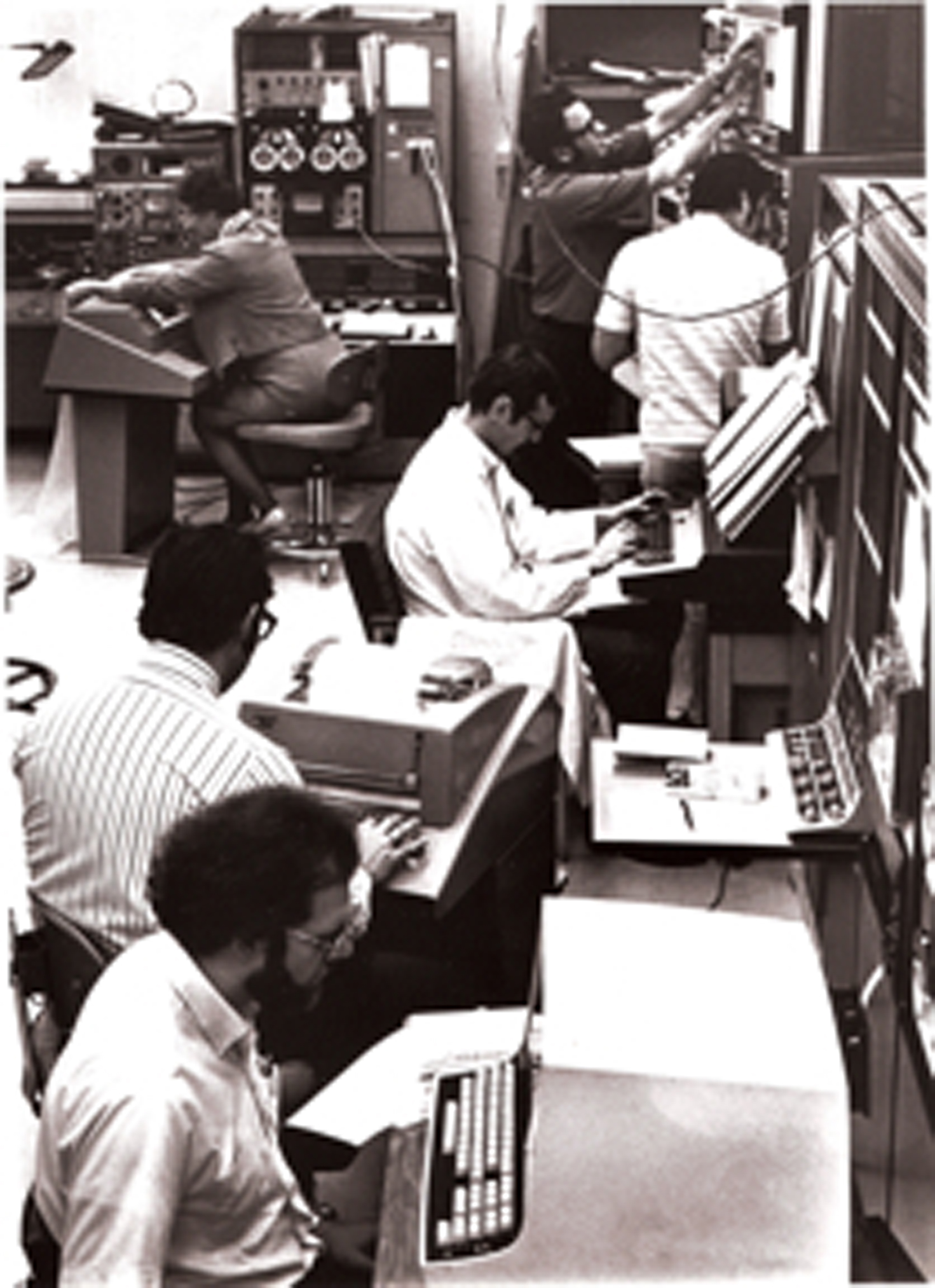
Figure 1. The Moore computer lab and personnel using the hybrid computer system. Foreground to background: the DEC PDP15, the analog–digital interface, and the analog computer. A LINC-8 computer is at the back.
Fortunately, Michael (Mike) Hines, who had joined my lab, was such a programmer; his background in physics gave him extensive knowledge of applied mathematics. Mike was able to program the hybrid system to produce HH impulses propagating at blinding speeds not only in an axon but also in branched cables. Once Fred Dodge, on a site visit, said that the computer’s display was too fast for him to follow – could we please slow the thing down?
The analog computer solved the HH equation for voltage, as well as for the HH variables “m,” “h,” and “n,” in a single compartment while the digital computer stored the results of each run, then switched (every 25 μs) to the next compartment, specifying new parameters and supplying the time-varying voltages of adjacent compartments using a modified Euler method. The hybrid’s speed was limited by the necessity of multiple iterations for complex morphologies. Fortunately the speed of digital machines was beginning to increase rapidly and they were also getting smaller. Therefore the lifetime of our enormous hybrid was short in our lab. Mike switched to a DEC PDP11 minicomputer where he could use much faster implicit integration along with variable time steps.
Computational Neuroscience Software
Two programmers, Mike Hines in my lab in the 1970s and James Bower at Cal Tech in the late 1980s, independently began developing software to run more sophisticated simulations. Hines’ software was developed to run in parallel with our lab’s experimental observations on the giant axon of the squid. Comparison of the simulations with experimental results guided experimental design and reassured us in our interpretation of observations. The first version of Mike’s software was called CABLE because it was limited to simulations of the squid giant axon. CABLE was then expanded to encompass the full morphology of a nerve cell and at that point was named NEURON 1 (Carnevale and Hines, 2006 ). Over some 30 years now, Mike has continued to develop this software into a widely used professional simulation environment. Although Mike developed NEURON in UNIX, he has ported it to run on Macintosh and Windows machines.
GENESIS 2 is also widely used simulation software from James Bower’s lab; it is UNIX-based, with a strong focus on neuronal networks. By the early 1990s some nine more simulation tools had become available.
Conclusion
One useful benchmark for computational neuroscience has been the ratio of the computer simulation time to the squid axon membrane’s time (5 ms) to generate and recover from an action potential. For the SEAC computer time of 1800 s in the 1950s, this ratio was 360,000. Now, in the first decade of the 21st century, notebook computers have dual processors running at about 3 GHz clock rates. Using the NEURON simulation environment, such machines can easily calculate the action potential about 10 times faster than the membrane does, over a million-fold increase in speed.
Even taking plotting into account, the time of calculation plus plotting is now in the neighborhood of the time interval between frames in a movie. Consequently, the human’s time to observe and interpret a simulation becomes the overall rate limiting step, obviating any need for further increases in computational speed for simulations of single neurons. The challenge now becomes one of making realistic simulations of neural networks.
In order to meet this challenge, simulation software must first of all be able to be ported to parallel machines (for example NEURON is now on the IBM Blue Gene). It is also imperative that the simulator be able to import detailed morphological descriptions of individual neurons. Beyond such importing, which can be done at present, exploitation of parallel computational power for realistic simulations of networks will require extensive, quantitative descriptions of neuronal properties: (1) the ion channel types, their densities and their distributions throughout each neuron; (2) the types and properties of intracellular calcium ion buffers, and their effect on intracellular spatial and temporal profiles of calcium concentration; (3) neurotransmitters, their release mechanisms, and modulation of release by activity; (4) neurotransmitter receptor types, properties, and sensitivity to modulation by other transmitters, hormones or activity; and (5) intracellular chemical reactions and signaling pathways which may, in turn, affect the release of transmitters and the sensitivity of receptors. It is a big order. Where will computational neuroscience be a decade from now, even as this information accrues? Predictions are impossible. Because the past decades of computational neuroscience have been such a thrilling ride, I can only suggest that, going forward, we should enjoy the show!
Conflict of Interest Statement
The author declares that the research was conducted in the absence of any commercial or financial relationships that could be construed as a potential conflict of interest.
Acknowledgments
I thank my former colleagues at Duke for their comments and suggestions for this article: Michael Hines, Ronald Joyner, Frank Starmer, Fidel Ramon, and Monte Westerfield. I also am most appreciative that other friends, Fred Dodge and Wilfrid Rall, helped me verify statements about their contributions to the field. I am sorry that I could not ask Dick FitzHugh and Don Perkel, now deceased, for their comments. I am deeply indebted to my wife and collaborator, Ann Stuart, for her invaluable help in preparing this article.
Footnotes
References
Bekey, G. A., and Paxson, B. (1957). “Analog simulation of nerve excitation,” in The 2nd National Simulation Conference, Houston, Texas, April 11–13.
Carnevale, N. T., and Hines, M. L. (2006). The NEURON Book. Cambridge, UK: Cambridge University Press.
Cole, K. S. (1968). Membranes, Ions, and Impulses. Berkeley, Los Angeles, CA: University of California Press.
Cole, K. S., Antosiewicz, H. A., and Rabinowitz, P. (1955). Automatic Computation of Nerve Excitation. National Bureau Standards Report 4238. Gaithersburg, MD: National Institute of Standards and Technology.
Cooley, J. W., and Dodge, F. A. (1966). Digital computer solutions for excitation and propagation of the nerve impulse. Biophys. J. 5, 583–599.
Dodge, F. A., and Cooley, J. W. (1973). Action potential of the motoneuron. IBM J. Res. Dev. 17, 219.
Dodge, F. A., and Frankenhaeuser, B. (1958). Membrane currents in isolated frog nerve fibre under voltage clamp conditions. J. Physiol. 143, 76–90.
Fishman, H. M. (1970). Direct and rapid description of the individual ionic currents of squid axon membrane by ramp potential control. Biophys. J. 9, 799–817.
FitzHugh, R. (1961). Impulses and physiological states in theoretical models of nerve membrane. Biophys. J. 1, 445–466.
FitzHugh, R. (1968). Motion picture of nerve impulse propagation using computer animation. J. Appl. Physiol. 25, 628–630.
FitzHugh, R., and Antosiewicz, H. A. (1959). Automatic computation of nerve excitation – detailed corrections and additions. J. Soc. Ind. Appl. Math. 7, 447–458.
Goldstein, S., and Rall, W. (1974). Changes of action potential shape and velocity for changing core conductor geometry. Biophys. J. 14, 731–757.
Joyner, R. W., and Moore, J. W. (1973). Computer controlled voltage clamp experiments. Ann. Biomed. Eng. 1, 368–380.
Joyner, R. W., Westerfield, M., Moore, J. W., and Stockbridge, N. (1978). A numerical method to model excitable cells. Biophys. J. 22, 155–170.
Moore, J. W., Joyner, R. W., Brill, M. H., and Waxman, S. G. (1978). Simulations of conduction in uniform myelinated fibers: relative sensitivity to changes in nodal and internodal parameters. Biophys. J. 21, 147–160.
Moore, J. W., and Ramon, F. (1974). On numerical integration of the Hodgkin and Huxley equations for a membrane action potential. J. Theor. Biol. 45, 249–273.
Moore, J. W., Ramon, F., and Joyner, R. (1975). Axon voltage-clamp simulations. I. Methods and tests. Biophys. J. 15, 11–24.
Rall, W. (1959). Branching dendritic trees and motoneuron membrane resistivity. Exp. Neurol. 1, 491–527.
Rall, W. (1967). Distinguishing theoretical synaptic potentials computed for different soma-dendritic distributions of synaptic input. J. Neurophysiol. 30, 1138–1168.
Rall, W., and Shepherd, G. (1968). Theoretical reconstruction of field potentials and dendrodendritic synaptic interactions in olfactory bulb. J. Neurophysiol. 31, 884–915.
Ramon, F., Joyner, R. W., and Moore, J. W. (1975). Propagation of action potentials in inhomogeneous axon regions. Fed. Proc. 34, 1357–1363.
Keywords: computational, neuroscience, simulations, Hodgkin–Huxley equations
Citation: Moore JW (2010) A personal view of the early development of computational neuroscience in the USA. Front. Comput. Neurosci. 4:20. doi: 10.3389/fncom.2010.00020
Received: 22 February 2010;
Paper pending published: 10 March 2010;
Accepted: 13 June 2010;
Published online: 07 July 2010
Edited by:
Nicolas Brunel, Centre National de la Recherche Scientifique, FranceReviewed by:
John Rinzel, New York University, USAIdan Segev, Hebrew University, Israel
Copyright: © 2010 Moore. This is an open-access article subject to an exclusive license agreement between the authors and the Frontiers Research Foundation, which permits unrestricted use, distribution, and reproduction in any medium, provided the original authors and source are credited.
*Correspondence: John W. Moore, Department of Neurobiology, Duke University Medical Center, Box 3209, Durham, NC 27710, USA. e-mail: moore@neuro.duke.edu