STDP in oscillatory recurrent networks: theoretical conditions for desynchronization and applications to deep brain stimulation

Introduction

High level of synchrony in neural tissue can be the cause of several diseases. For example, Parkinson’s disease is characterized by high level of neuronal synchrony in the thalamus and in the basal ganglia. In opposition, the same neural tissues in healthy conditions have been shown to fire in an asynchronous way (Nini et al., 1995). The Parkinsonian resting tremor (3–6 Hz) is not only related to the subcortical oscillations (Pare et al., 1990), but has been recently shown to be driven by those oscillations (Smirnov et al., 2008; Tass et al., 2010). In addition, the extent of akinesia and rigidity is closely related to synchronized neuronal activity in the beta band (8–30 Hz) (Kuhn et al., 2006).

A standard treatment for patients with Parkinson’s disease is to chronically implant an electrode typically in the sub-thalamic nucleus (STN) and perform a high-frequency (>100 Hz) deep brain stimulation (HF-DBS) (Benabid et al., 1991, 2009). Although HF-DBS delivered to the STN is able to reduce tremor, akinesia, and rigidity, this type of stimulation, which was found empirically, does not cure the cause of the tremor. It merely silences the targeted neurons during the stimulation but as soon as the stimulation is turned off, the tremor restarts instantaneously, whereas akinesia and rigidity revert back within minutes to half an hour (Temperli et al., 2003).

Recently, other types of stimulation (Tass, 1999, 2003; Tass and Majtanik, 2006; Hauptmann and Tass, 2007, 2009; Tass and Hauptmann, 2007) have been proposed which are not designed to ‘silence’ the neurons during the stimulation but rather reshape the network architecture in a way that long-lasting desynchronizing effects occur which outlast the offset of stimulation. This approach relies on two properties or requirements of the neural tissue. First, the network dynamics must elicit bistability such that both the synchronized and the desynchronized state are stable (see Figure 1A). Second, there must exist a stimulation that (momentarily) destroys the stability of the synchronous state such that the network is driven into the desynchronized stable state (see Figure 1B).

FIGURE 1

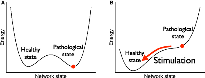
Figure 1. Bistability for therapeutical stimulation. (A) Before stimulation, both the pathological state (strong weights, high neuronal synchrony) and the healthy state (weak weights, low neuronal synchrony) are stable, i.e., they are local minima of an abstract energy function. (B) During stimulation, the pathological state becomes unstable and the network is driven towards the healthy state. After stimulation has stopped, the network stays in the healthy state.

Unfortunately, most of the work that follows this idea of therapeutical stimulation is based on numerical simulations ( Tass and Majtanik, 2006; Hauptmann and Tass, 2007, 2009; Tass and Hauptmann, 2007) and only very little has been done analytically (Maistrenko et al., 2007) in order to understand what are the crucial parameters that lead to the two above requirements. Here we consider a recurrent network model that is sufficiently simple to be treated analytically but still captures the desired properties.

Concretely, we consider in this paper a network dynamics that acts on two different time scales. On a short-time scale, neurons integrate the inputs from neighboring neurons and fire periodically. On a longer time scale, synapses can change their strength and hence influence the overall level of synchrony. In principle the above mentioned requirement on bistability can be present in either the neuronal dynamics (short-time scale) or the synaptic dynamics (longer time scale). Since we are aiming for long-lasting effects, we focus on the bistability in the synaptic dynamics. More precisely, we consider a synaptic plasticity learning rule that depends on the precise timing of the action potentials of the pre- and postsynaptic neurons. This form of plasticity called spike-timing dependent plasticity (STDP) (Gerstner et al., 1996b; Markram et al., 1997; Bi and Poo, 1998) enhances synapses for which the presynaptic spike precedes the postsynaptic one and decreases the synaptic strength when the timing is reversed (see Figure 3A).

Regarding the stimulation itself, several candidates have been proposed. For example, it has been shown that a patterned, multi-site and timed-delayed stimulation termed as coordinated reset (CR) stimulation (Tass, 2003) which forces sub-populations to fire in a precise sequence generates transiently a nearly uniform phase distribution. In fact, long-lasting desynchronizing effects of CR stimulation have been verified in rat hippocampal slice rendered epileptic by magnesium withdrawal (Tass et al., 2009).

In the present study, we do not focus on a precise stimulation but rather assume that there exists a stimulation that desynchronizes transiently a given population. Furthermore a given stimulation rarely affects the whole population which fires in a pathological way but only part of it. So we consider two populations. An input population which is affected by the stimulation (see Figure 2A) and a recurrent population with plastic synapses which is driven by the input population.

FIGURE 2

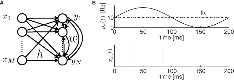
Figure 2. (A) Network architecture. (B) The input spike train x_k(t) (bottom) of neuron k has an instantaneous firing rate ρ_k(t) (top) which is oscillating around an averaged firing rate

In order to calculate the expected weight change in the recurrent network, we need to get an expression for the spiking covariance of this recurrent population. This technical step has been achieved by Hawkes (1971) and used by Gilson et al. (2009a,b) in the context of recurrent network with STDP. The present study extends the work of Gilson et al. (2009b) to the case of oscillatory inputs and highlights the conditions for which the network elicits bistability.

Materials and Methods

Neuronal Dynamics

Let us consider an input population consisting of M neurons and a recurrent population containing N neurons (see Figure 2A). Let x(t) = (x₁(t),…,x_M(t)) denote the input spike trains at time t with being the Dirac delta spike train of the j^th input neuron. Let x^t = {x(s), 0 ≤ s < t} describe the whole input spike pattern from 0 to t. Similarly, let y(t) = (y₁(t),…,y_N(t)) denote the spike trains of the recurrent (or output) population, i.e., denotes the Dirac delta spike train of the i^th neuron in the recurrent population at time t. y^t = {y(s), 0 ≤ s < t} represents the output spike train from 0 to t.

Let us assume that the input spike trains x(t) have instantaneous firing rates ρ(t) = (ρ₁(t),…,ρ_M(t)) = 〈x(t)〉_x(t) which are assumed to be periodic (i.e., ρ(t) = ρ(t + T), see Figure 2B) and a spatio-temporal covariance matrix ΔC(τ) given by

where is the mean firing rate averaged over one period T. Note that the input covariance matrix ΔC(τ) has an atomic discontinuity at τ = 0, i.e., Let denote the membrane potential of all the neurons in the recurrent population (see the Spike-Response Model in Gerstner and Kistler, 2002):

where the superscript є denotes a convolution¹ with the EPSP kernel є(s), i.e., and Without loss of generality, we will assume that the EPSP kernel is such that More precisely, we take є(s) = (τ − τ_s)⁻¹ (exp(−s/τ) − exp(−s/τ_s))Θ(s), where Θ(s) is the Heaviside step function. The N × M matrix h denotes the weight matrix between the input and the recurrent population. w is a N × N matrix denoting the recurrent weights (see Figure 2A).

In this model, output spikes are generated stochastically, i.e., the higher the membrane potential the more likely a spike will be emitted. Formally a spike is generated in neuron i at time t with an instantaneous probability density given by

where with denoting the expected membrane potential of neuron i averaged over a period T, and its vectorial representation. The expected output firing rates at time t is therefore given by

where D′ = diag(g′(ū)). Note that from Eq. 2, the averaged expected membrane potential ū can be expressed as where is the averaged output firing rate. Combining those two expressions, we get a self-consistent equation for the averaged output firing rate

Note that if the transfer function g(u) is linear, i.e., g(u) = u, we have . Let denote the amplitude of the oscillation in the recurrent population:

where denotes the amplitude of the input oscillation and Since Δν(t) appears on the l.h.s of Eq. 6 and in a convolved form on the r.h.s, we can Fourier transform this equation in order to express explicitly the amplitude of the oscillation in the recurrent population as a function of the angular frequency ω:

where 𝟙 denotes the N×N identity matrix, The tilde symbol denotes the Fourier transform, i.e., The recurrent population is said to be highly synchronous if is large where ω₀ = 2π/T. It is well known that coupled Kuramoto oscillators do synchronize if the coupling exceeds a certain threshold (Kuramoto, 1984)². Here, because we do not consider phase oscillators (such as the Kuramoto oscillators) as neuronal models, this result does not apply directly. However, as we can see in Eq. 7 the stronger the recurrent weights w, the bigger the amplitude of the output oscillation Let ΔQ(τ) be the spiking covariance matrix of the recurrent population:

Note that ΔQ(τ) contains an atomic discontinuity at τ = 0, i.e., ΔQ(0) = Dδ(0) with As can be seen in “Spiking Covariance Matrices” in Appendix, it is easier to calculate this covariance matrix in the frequency domain, i.e., rather than in the time domain. So the Fourier transform of this output covariance matrix yields

where denotes the Fourier transform of the input covariance matrix.

Synaptic Dynamics

In the previous section, we assumed that all the weights were constant in order to calculate the output covariance matrix. Let us now allow the recurrent weights w to change very slowly (w.r.t. the neuronal dynamics) and keep the input weights h fixed. Because of this separation of time scales, we can still use the results derived so far.

In the same spirit as Kempter et al. (1999), Gerstner and Kistler (2002), Gilson et al. (2009b), we can express the weight change as a Volterra expansion of both the pre- and postsynaptic spike trains. If we keep terms up to second order we get for all i ≠ j:

Since we do not allow for self-coupling, we will set a^pre(w) (and a^post(w)) denote the weight change induced by a single presynaptic (resp. postsynaptic) spike. W(s,w) denotes the STDP learning window (see Figure 3A) and its Fourier transform (see Figure 3B):

FIGURE 3

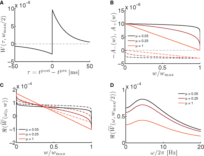
Figure 3. Properties of the STP learning window. (A) STDP learning window evaluated at w = w_max/2. τ₊ = 17 ms, τ₋ = 34 ms. (B) LTP factor A₊(w) (solid lines) and LTD factor A₋(w) (dot-dashed lines) as a function of the weight. See Eqs 12 and 13. (C) Real part of the Fourier transformed learning window (solid lines) as a function of the weight w at the angular frequency ω₀ = 2π/T, with T = 200 ms. Dot-dashed lines: integral of the learning window as a function of the weight w. (D) Real part of the Fourier transformed learning window as a function of the oscillation frequency f = ω/2π.

Consistently with the modeling literature on STDP (van Rossum et al., 2000; Gütig et al., 2003; Morrison et al., 2007, 2008) both the potentiation factor and the depression factor are assumed to depend on the weight. Here, the precise dependence on the weights corresponds to the one used by Gütig et al. (2003):

where the parameter controls the dependence upon the weight. If μ → 0, the rule is additive and therefore independent on the weight w. Conversely, if μ → 1, the rule becomes multiplicative. Unless specified otherwise, we set μ = 0.05. In addition to this learning rule, hard bounds for the weights (0 ≤ w_ij ≤ w_max, ∀i ≠ j) are required if the factors a^pre(w) and a^post(w) are independent of the weights (which we will assume here) or if they do not contain implicit soft bounds. Because of the separation of time scales assumption, we can replace the recurrent weights by their expected value averaged over one period T, i.e., and get:

where denotes the area under the STDP curve for a given weight w_ij. Since it is easier to express this covariance matrix in the frequency domain we can rewrite Eq. 14 (in matrix form) as³:

where is given by Eq. 9 and the ‘◦’ operator denotes the pointwise matrix multiplication (also known as the Hadamard product). The operator φ sets to zero the diagonal elements and keep the off-diagonal elements unchanged. This implements the fact that we are not allowing autapses. 1 = (1,…,1) is a vector containing N ones.

Sinusoidal Inputs

Let us now assume that the input population is exciting the recurrent population with independent Poisson spike trains of sinusoidal intensity where ω₀ = 2π/T is the angular frequency. Because of the independence assumption, the input correlation matrix yields

and its Fourier transform yields

By using this expression of the input correlation, we get an explicit expression for the output covariance matrix (see Eq. 9) which can be approximated as:

with see Eq. 7. This approximation is valid in the limit of large networks (M >> 1, N >> 1) where the terms involving diagonal matrices can be neglected. Indeed the term which depends on scales as M⁻¹ and the term which depends on scales as N⁻¹ if the output firing rate is kept constant. For a detailed discussion, see Kempter et al. (1999), Gilson et al. (2009b). By inserting Eq. 18 into Eq. 15, we get:

where ℜ(x) takes the real part of x. Here, we assumed that both a^pre and a^post are independent of the recurrent weights w. Furthermore, if g(u) = u, then the diagonal matrix D′ = 𝟙 (which is present in and ) is independent of the recurrent weights w.

Results

So far, we derived analytically the neuronal dynamics of a recurrent population that is stimulated by an oscillatory input. Furthermore we calculated the synaptic dynamics of such a recurrent network when synapses are governed by STDP. This rich synaptic dynamics has several interesting properties that are relevant for therapeutical stimulation and that we describe below.

Firstly, under some conditions that will be detailed below, the synaptic dynamics can elicit bistability (see Figures 4A,B). Concretely, if synapses are initialized above a critical value w*, they will grow and reach the upper bound w_max. Conversely, if they are initialized below w*, they will decrease down to their minimal value. As a consequence, because the amplitudes of the oscillations in the recurrent population depend on the strength of the recurrent weights (see Eqs 7 and 22), then this bistability at the level of the weights implies a similar bistability at the level of the oscillation amplitude of the recurrent population (see Figure 4C).

FIGURE 4

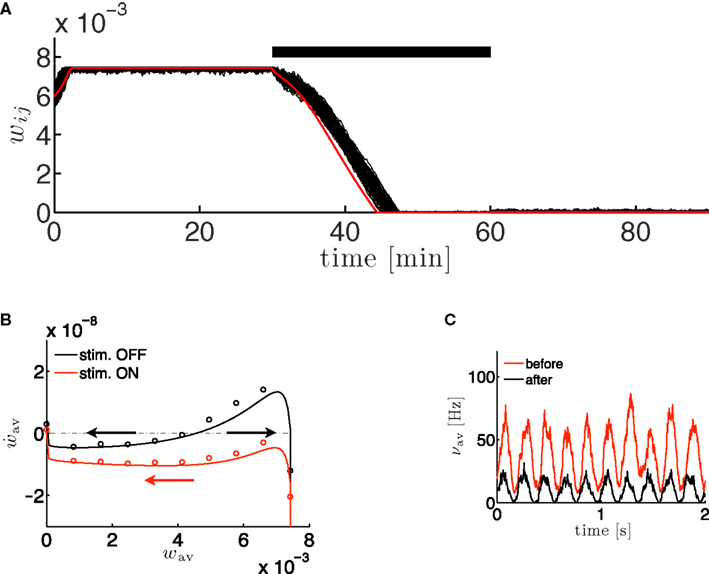
Figure 4. The bistability of the recurrent network with STDP can be exploited for therapeutical stimulation. (A) Evolution of the recurrent weights w_ij as a function of time for M = N = 100. Black lines: individual weights in a numerical simulation. Red line: Evolution of the averaged recurrent weight obtained analytically (see Eq. 20) Thick black line: extent of stimulation. (B) Phase plane analysis of the averaged weight w_av. In the presence of a stimulation that annihilates the oscillations in the input (red: stim. ON, Δρ₀ = 0 Hz) the averaged recurrent weight tends towards the lower bound w_min = 0. In the absence of the stimulation (black: stim. OFF, Δσ₀ = 10 Hz), w increases up to the upper bound if it is bigger than a critical value w* ≃ 4.5 · 10⁻³. Black and red lines: analytical result, black and red circles: numerical simulation. (C) Evolution of the averaged output firing rate before (red) and after (black) stimulation. The parameters are: τ = 10 ms, τ_s = 0 ms, a^pre = 0, a^post = − 1.7·10⁻⁶, h = 1/N, . Parameters of the learning window same as in Figure 3.

Secondly, the presence of the desynchronizing stimulation, which is modeled by setting the amplitude of the oscillatory input Δρ₀ to 0, removes the bistability and pushes all the weights to their minimal value (see Figures 4A,B). Once the stimulation is removed the recurrent weights stay at their minimum value because it is a fixed point of the dynamics.

Homogeneous Case

Because the analysis of the non-linear dynamical system given by Eq. 19 can be challenging, let us consider the dynamics of the averaged recurrent weight in the homogeneous case.

More precisely, we assume here that all the mean input firing rates are close to their averaged value and that the input weights h_ij are close to their averaged value If we further assume that the initial values of the recurrent weights w_ij(0) are close to w_av, then, as long as the individual weights do not diverge too much, the dynamics of the averaged recurrent weight can be approximated as⁴:

If the transfer function is linear, i.e., g(u) = u, the averaged output firing rate and the oscillation amplitude of the recurrent population can be approximated as:

with The dynamics of the averaged recurrent weight w_av given by Eq. 20 is remarkably consistent with numerical simulations performed with spiking neurons (see Figures 4A,B). The small discrepancy between the numerics and analytics can be attributed to two factors. First, Eq. 20 assumes the limit of large networks, i.e., N, M → ∞ whereas in the numerical simulations, we used N = M = 100. Secondly, Eq. 20 is valid in the limit of small recurrent weights, i.e., w_av << 1/N (here we used Nw_max = 0.75). As we can see on Figure 4B, the smaller averaged weights w_av, the better the correspondence between the numerical simulation and the analytical calculations. Even, for large recurrent weights (w_av ≃ w_max), the discrepancy between numerics and analytics is remarkably small.

Conditions for Bistability

So far, we discussed a scenario in which the stimulation effectively acted as a therapeutical stimulation because it shifted the network state from the highly synchronous (and therefore pathological) state to the low synchronous state. In order to have this property, the network must satisfy two conditions:

• C1. Bistability condition. In the absence of stimulation, the network must elicit bistability such that both the synchronized and the desynchronized state are stable. Formally this gives

• C2. Desynchronizing stimulation condition. In the presence of a desynchronizing stimulation, the highly synchronous state looses its stability and the network is driven to the low synchronous state. This can be expressed as:

In order to keep the discussion reasonably simple, let us make several assumptions. First, let us consider the near-additive learning rule i.e., μ ≃ 0. Indeed in the case of a multiplicative learning rule (i.e., μ ≫ 0), the potentiation factor A₊(w) and the depressing factor A₋(w) have a strong stabilization effect and therefore no bistability can be expected; see Figure 5A with μ = 0.5. This is consistent with the findings of Gütig et al. (2003) who showed that there is a symmetry breaking in feedforward networks with weight-dependent STDP for μ bigger than a critical value.

FIGURE 5

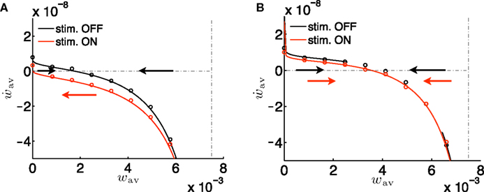
Figure 5. Conditions for the absence of bistability. (A) Phase plane analysis similar to the one in Figure 4B, but for μ = 0.5. There is no bistability because the weight-dependent factors A₋(w) and A₊(w) play here a dominant role. (B) Same as in Figure 4B, but with an overall negative learning window, i.e., all parameters identical except and a^post = 0.1·10⁻⁵.

With this additivity assumption and the linear transfer function assumption (g(u) = u), the averaged recurrent weight dynamics can be simply expressed from Eq. 20 combined with Eqs 21 and 22:

where and are constant and do not depend on the averaged recurrent weight w_av.

Another greatly simplifying assumption is to consider the low oscillatory frequency regime, i.e., ω₀τ << 1 which gives . 1.

Bistability condition C1

With these assumptions, the fixed point expressed in the bistability condition C1 yields

Because this fixed point has to be between 0 and w_max, we have or equivalently

If we push the low-frequency assumption further such that ω₀τ₊ << 1 and τ₋ << 1, we have (see Figure 3C). In this case, Eq. 25 yields a simple necessary condition: a^pre + a^post and the integral of the learning window must be of opposite sign:

Finally, the fact that the fixed point must be unstable (see condition C1), we have which gives By using the expression of given in Eq. 24 we have α₂ + α₃ > 0 and therefore with Eq. 26, we get:

which is consistent with the parameters used in Figures 3 and 4. Note that in Figure 5B, we violated this condition and as a consequence the bistability property is lost.

Desynchronization stimulation condition C2

In the presence of the desynchronization stimulation (i.e., Δρ_av = 0), the condition C2 implies that α₁(1 − Nw_av) + α₂ < 0. Because α₁ < 0 (see Eq. 27), this condition is satisfied for all w_av if α₁(1 − Nw_max) + α₂ < 0. By introducing the values for α₁ and α₂, we get:

By combining the conditions C1 and C2, α₁ has to obey

In summary, in order to satisfy both conditions C1 and C2, the learning rule must be nearly additive (μ ≃ 0), the learning window must be overall positive and the sum of the coefficients tuning the effect of single spikes (a^pre and a^post) must be negative with upper and lower bounds set by Eq. 29.

Note that the bistability conditions derived above are valid for the averaged recurrent weight and do not apply for the individual weights of the recurrent population. As a consequence, this bistability condition does not necessarily imply a bimodal weight distribution. Indeed, if we consider the same set-up as in Figure 4, but draw the initial weights from a uniform distribution, between 0 and w_max, then all the weights will eventually settle into a unimodal distribution, around w = 0 (data not shown).

A bimodal weight distribution has been shown to occur in recurrent networks with additive STDP learning rule (Gilson et al., 2009b) favoring neurons that receive correlated inputs. For the sake of simplicity we considered in the simulations identical (and uncorrelated) inputs but the recurrent weight dynamics described by Eq. 15 remains valid for any type of inputs.

Discussion

In this paper, we developed a model of a recurrent network with plastic synapses that is sufficiently simple to be treated analytically but that still yields the desired properties. In particular, we showed that when (a) the STDP learning rule is near additive and (b) the learning window is overall positive and (c) the terms in the learning rule involving single spikes (a^pre + a^post) have a depressing effect (within some bounds), then a desynchronizing stimulation favors long-term depression in the recurrent synapses and therefore drives the network from a highly synchronous state to a desynchronous state. In this way, our study confirms previously performed simulation studies (Tass and Majtanik, 2006; Hauptmann and Tass, 2007, 2009; Tass and Hauptmann, 2007) and, in particular, contributes to a theoretically sound foundation for the development of desynchronizing and, especially, anti-kindling brain stimulation techniques.

The concept of anti-kindling, i.e., of an unlearning of pathological synchrony and connectivity by desynchronizing stimulation, has been introduced by Tass and Majtanik (2006). For this, STDP was incorporated into a generic network of phase oscillators, and both kindling and anti-kindling processes were studied numerically. To approach a more microscopic level of description, a network of bursting neurons has been introduced as a simple model for an oscillatory population in the STN (Tass and Hauptmann, 2006, 2007; Hauptmann and Tass, 2007). With this model different aspects of kindling and anti-kindling processes have been studied numerically, such as the effect of inhibition vs. excitation (Hauptmann and Tass, 2007), the impact of weak and particularly short stimuli (Tass and Hauptmann, 2006), post-stimulus transients and cumulative stimulation effects (Hauptmann and Tass, 2009) as well as the differential effects of different sorts of desynchronizing stimulation protocols (Tass and Hauptmann, 2009). These questions are highly relevant for the clinical application of desynchronizing stimulation to the therapy of diseases with abnormal synchrony, e.g., Parkinson’s disease. In forthcoming studies, more microscopic models will be studied. However, apart from this type of numerical simulation analysis, we aim at establishing a thorough, analytical framework for the anti-kindling concept. As a first step into that direction, we presented here an analytical analysis of a simple network model which we validated by numerical analysis.

Different types of neurons and, hence, different target areas in the brain may be associated with different types of STDP learning rules. Accordingly, brain stimulation approaches might be optimized with respect to a particular type of STDP learning rule in order to achieve superior therapeutic effects.

This work is not the first one to treat STDP in oscillatory recurrent network. Karbowski and Ermentrout (2002) consider neurons as formal phase oscillators and therefore do not consider spiking neurons as such. Furthermore Karbowski and Ermentrout (2002) consider a learning window with identical potentiation and depression time constants which limits the potential output of the study. Maistrenko et al. (2007) describe as well neurons as phase oscillators, but they allow potentiation and depression time constants to be different. Interestingly they find multistability depending on those time constants and on the weight upper bound. Morrison et al. (2007) consider a STDP learning rule with multiplicative depression and power-law dependence for potentiation and showed numerically that this STDP rule decouples synchronous inputs from the rest of the network.

Our present model can be seen as an extension of the work of Gilson et al. (2009a,b) in several aspects. First, and most importantly, we consider here oscillatory input whereas Gilson et al. (2009b) assume stationary inputs. In this way we are able to discuss the conditions on the learning parameters to get a bistable regime with high and low synchrony. Secondly, our approach does not require to calculate the inverse Fourier transform of the spiking covariance matrix. In this way we do not need to make the (unrealistic) assumption that the EPSP time constant is much smaller than potentiation time constant in the learning window. Finally, we consider a larger class of neuronal model since we do not restrict ourself to linear neurons, but consider instead (locally linearized) non-linear neurons.

There are several ways in which we can extend the present model. It is known that propagation delays play an important role in the neuronal synchrony (Gerstner et al., 1996a; Cassenaer and Laurent, 2007; Lubenov and Siapas, 2008). Our framework can be easily extended to incorporate those propagation delays. A systematic analysis of the influence of those delays is out of the scope of the current study but would be definitely relevant. According to the arguments of Lubenov and Siapas (2008), one could expect that the bigger the synaptic delays, the stronger the effective amount of depression. This can potentially change the stability of highly synchronous states.

Another way to extend the current model is to consider learning rules that depend on high order statistics of the pre- and postsynaptic neuron. For example, it is known that a triplet learning rule which considers 1 pre- and 2 postsynaptic spikes (Pfister and Gerstner, 2006a,b; Clopath et al., 2010) is more realistic in terms a reproducing experimental data than the pair-based STDP considered here. Another extension would be to consider second order terms in the Taylor expansion of the transfer function. Both of those extensions would require a substantial amount of work since the results of Hawkes (1971) could not be used anymore.

Appendix

Spiking Covariance Matrices

Input–Output Covariance Matrix

In order to express the output spiking covariance matrix ΔQ as a function of the input spiking covariance matrix ΔC, we need first to define the input–output covariance matrix ΔP:

By rewriting the average involved here and by using Eqs 1, 2, and 3, the input–output covariance matrix can be expressed in a self-consistent way as:

where D′ = diag(g′(ū)) is a diagonal matrix with Here the є superscript denotes as before the convolution with є(s), i.e., and In order to get an explicit expression of this input–output covariance matrix, we can Fourier transform Eq. 31 and therefore turn the convolution into a product in the angular frequency domain ω:

where 𝟙 denotes the N × N identity matrix, As before the tilde symbol denotes the Fourier transform, i.e.,

Output Covariance Matrix

We recall here for convenience the definition of the output covariance matrix (see Eq. 8):

For τ ≥ 0, we have:

with D = diag(g(ū)). Since the above identity is only valid for τ ≥ 0, we can not simply Fourier transform this expression and extract the output covariance matrix in frequency domain. We will use here the same method as proposed by Hawkes (1971). Let B(τ) be a supplementary matrix defined as:

Because this supplementary matrix is defined ∀τ, we can Fourier transform it and express the output covariance matrix in frequency domain:

From the definition of the output covariance matrix ΔQ(τ) in Eq. 33, we have ΔQ(−τ) = ΔQ^T(τ) and hence By using this property and the fact that , we have

or, equivalently

In order to express Hawkes (1971) used a regularity argument which goes as follows. Let us assume є(t) and |B(t)| are bounded as follows:

We can show that both (and hence ) is regular for ℑ(ω) < η and is regular for ℑ(ω) > −η. Let H(ω) be defined as the l.h.s. of Eq. 38 for ℑ(ω) < η and the r.h.s of Eq. 38 when ℑ(ω) > −η. In this way H(ω) is regular everywhere and since we have H(ω) → 0 when |ω| → ∞, we know from Liouville’s theorem that H(ω) = 0. In particular, from the r.h.s of Eq. 38, we can express the supplementary matrix as:

If we insert this expression back into Eq. 36, we get:

Conflict of Interest Statement

The authors declare that the research was conducted in the absence of any commercial or financial relationships that could be construed as a potential conflict of interest.

Acknowledgments

We thank Oleksandr Popovych for fruitful discussions. Jean-Pascal Pfister has been supported by the Wellcome Trust.

Footnots

1. ^Each component of x^є(t) is convoluted with є(s), i.e., k = 1,…,M.
2. ^Other types of coupled oscillators have the property that strong coupling may destroy synchronization under particular conditions, e.g., in a population of identical diffusively coupled Rössler oscillators (Heagy et al., 1995) or in a system of two coupled chaotic non-invertible maps (Maistrenko et al., 1998). However, such models do not apply to the pathophysiology considered here. Furthermore, these models do not contain STDP, and it remains to be shown whether such phenom-ena persist in the presence of STDP.
3. ^The last term in Eq. 15 is obtained by defining then taking the Fourier transform and finally taking the inverse Fourier transform and evaluate it at t = 0.
4. ^Note that from the definition of the Fourier transform we have

References

Benabid, A., Chabardes, S., Mitrofanis, J., and Pollak, P. (2009). Deep brain stimulation of the subthalamic nucleus for the treatment of Parkinson’s disease. Lancet Neurol. 8, 67–81.

Pubmed Abstract | Pubmed Full Text | CrossRef Full Text

Benabid, A., Pollak, P., Gervason, C., Hoffmann, D., Gao, D., Hommel, M., Perret, J., and De Rougemont, J. (1991). Long-term suppression of tremor by chronic stimulation of the ventral intermediate thalamic nucleus. Lancet 337, 403.

Pubmed Abstract | Pubmed Full Text | CrossRef Full Text

Bi, G., and Poo, M. (1998). Synaptic modifications in cultured hippocampal neurons: dependence on spike timing, synaptic strength, and postsynaptic cell type. J. Neurosci. 18, 10464–10472.

Pubmed Abstract | Pubmed Full Text

Cassenaer, S., and Laurent, G. (2007). Hebbian STDP in mushroom bodies facilitates the synchronous flow of olfactory information in locusts. Nature 448, 709–713.

Pubmed Abstract | Pubmed Full Text | CrossRef Full Text

Clopath, C., Büsing, L., Vasilaki, E., and Gerstner, W. (2010). Connectivity reflects coding: a model of voltage-based STDP with homeostasis. Nat. Neurosci. 13, 344–352.

Pubmed Abstract | Pubmed Full Text | CrossRef Full Text

Gerstner, W., Kempter, R., van Hemmen, J., and Wagner, H. (1996a). A neuronal learning rule for sub-millisecond temporal coding. Nature 383, 76–78.

Pubmed Abstract | Pubmed Full Text | CrossRef Full Text

Gerstner, W., and Kistler, W. K. (2002). Spiking Neuron Models. Cambridge UK: Cambridge University Press.

Gerstner, W., van Hemmen, J. L., and Cowan, J. D. (1996b). What matters in neuronal locking. Neural. Comput. 8, 1653–1676.

Pubmed Abstract | Pubmed Full Text | CrossRef Full Text

Gilson, M., Burkitt, A., Grayden, D., Thomas, D., and van Hemmen, J. (2009a). Emergence of network structure due to spike-timing-dependent plasticity in recurrent neuronal networks iii: partially connected neurons driven by spontaneous activity. Biol. Cybern. 101, 411–426.

CrossRef Full Text

Gilson, M., Burkitt, A., Grayden, D., Thomas, D., and van Hemmen, J. (2009b). Emergence of network structure due to spike-timing-dependent plasticity in recurrent neuronal networks iv: structuring synaptic pathways among recurrent connections. Biol. Cybern. 101, 427–444.

CrossRef Full Text

Gütig, R., Aharonov, R., Rotter, S., and Sompolinsky, H. (2003). Learning input correlations through non-linear temporally asymmetric hebbian plasticity. J. Neurosci. 23, 3697–3714.

Pubmed Abstract | Pubmed Full Text

Hauptmann, C., and Tass, P. A. (2007). Therapeutic rewiring by means of desynchronizing brain stimulation. Biosystems 89, 173–181.

Pubmed Abstract | Pubmed Full Text | CrossRef Full Text

Hauptmann, C., and Tass, P. A. (2009). Cumulative and after-effects of short and weak coordinated reset stimulation: a modeling study. J. Neural Eng. 6, 016004.

Pubmed Abstract | Pubmed Full Text | CrossRef Full Text

Hawkes, A. G. (1971). Spectra of some self-exciting and mutually exciting processes. Biometrika 58, 83–90.

CrossRef Full Text

Heagy, J., Pecora, L., and Carroll, T. (1995). Short wavelength bifurcations and size instabilities in coupled oscillator systems. Phys. Rev. Lett. 74, 4185–4188.

Pubmed Abstract | Pubmed Full Text | CrossRef Full Text

Karbowski, J., and Ermentrout, G. (2002). Synchrony arising from a balanced synaptic plasticity in a network of heterogeneous neural oscillators. Phys. Rev. E 65, 31902.

CrossRef Full Text

Kempter, R., Gerstner, W., and van Hemmen, J. L. (1999). Hebbian learning and spiking neurons. Phys. Rev. E 59, 4498–4514.

CrossRef Full Text

Kuhn, A., Kupsch, A., Schneider, G., and Brown, P. (2006). Reduction in subthalamic 8–35 Hz oscillatory activity correlates with clinical improvement in Parkinson’s disease. Eur. J. Neurosci. 23, 1956.

Pubmed Abstract | Pubmed Full Text | CrossRef Full Text

Kuramoto, Y. (1984). Chemical Oscillations, Waves, and Turbulence. Berlin, Heidelberg, New York: Springer, 68–77.

Lubenov, E., and Siapas, A. (2008). Decoupling through synchrony in neuronal circuits with propagation delays. Neuron 58, 118–131.

Pubmed Abstract | Pubmed Full Text | CrossRef Full Text

Maistrenko, Y., Maistrenko, V., Popovich, A., and Mosekilde, E. (1998). Transverse instability and riddled basins in a system of two coupled logistic maps. Phys. Rev. E 57, 2713–2724.

CrossRef Full Text

Maistrenko, Y. L., Lysyansky, B., Hauptmann, C., Burylko, O., and Tass, P. A. (2007). Multistability in the kuramoto model with synaptic plasticity. Phys. Rev. E 75, 66207.

CrossRef Full Text

Markram, H., Lübke, J., Frotscher, M., and Sakmann, B. (1997). Regulation of synaptic efficacy by coincidence of postysnaptic AP and EPSP. Science 275, 213–215.

Pubmed Abstract | Pubmed Full Text | CrossRef Full Text

Morrison, A., Aertsen, A., and Diesmann, M. (2007). Spike-timing dependent plasticity in balanced random networks. Neural. Comput. 19, 1437–1467.

Pubmed Abstract | Pubmed Full Text | CrossRef Full Text

Morrison, A., Diesmann, M., and Gerstner, W. (2008). Phenomenological models of synaptic plasticity based on spike timing. Biol. Cybern. 98, 459–478.

Pubmed Abstract | Pubmed Full Text | CrossRef Full Text

Nini, A., Feingold, A., Slovin, H., and Bergman, H. (1995). Neurons in the globus pallidus do not show correlated activity in the normal monkey, but phase-locked oscillations appear in the MPTP model of Parkinsonism. J. Neurophysiol. 74, 1800.

Pubmed Abstract | Pubmed Full Text

Pare, D., Curro’Dossi, R., and Steriade, M. (1990). Neuronal basis of the Parkinsonian resting tremor: a hypothesis and its implications for treatment. Neuroscience 35, 217–226.

Pubmed Abstract | Pubmed Full Text | CrossRef Full Text

Pfister, J.-P., and Gerstner, W. (2006a). “Beyond pair-based STDP: a phenomenological rule for spike triplet and frequency effects,” in Advances in Neural Information Processing Systems 18, eds Y. Weiss, B. Schölkopf, and J. Platt (Cambridge: MIT Press), 1083–1090.

Pfister, J.-P., and Gerstner, W. (2006b). Triplets of spikes in a model of spike timing-dependent plasticity. J. Neurosci. 26, 9673–9682.

CrossRef Full Text

Smirnov, D., Barnikol, U., Barnikol, T., Bezruchko, B. P., Hauptmann, C., Bührle, C., Maarouf, M., Sturm, V., Freund, H. J., and Tass, P. A. (2008). The generation of Parkinsonian tremor as revealed by directional coupling analysis. Europhys. Lett. 83, 20003.

CrossRef Full Text

Tass, P. A. (1999). Phase Resetting in Medicine and Biology: Stochastic Modelling and Data Analysis. Berlin: Springer.

Tass, P. A. (2003). A model of desynchronizing deep brain stimulation with a demand-controlled coordinated reset of neural subpopulations. Biol. Cybern. 89, 81–88.

Pubmed Abstract | Pubmed Full Text | CrossRef Full Text

Tass, P. A., and Hauptmann, C. (2006). Long-term anti-kindling effects induced by short-term, weak desynchronizing stimulation. Nonlinear Phenomena Complex Syst. 9, 298.

Tass, P. A., and Hauptmann, C. (2007). Therapeutic modulation of synaptic connectivity with desynchronizing brain stimulation. Int. J. Psychophysiol. 64, 53–61.

Pubmed Abstract | Pubmed Full Text | CrossRef Full Text

Tass, P. A., and Hauptmann, C. (2009). Anti-kindling achieved by stimulation targeting slow synaptic dynamics. Restor. Neurol. Neurosci. 27, 589–609.

Pubmed Abstract | Pubmed Full Text

Tass, P. A., and Majtanik, M. (2006). Long-term anti-kindling effects of desynchronizing brain stimulation: a theoretical study. Biol. Cybern. 94, 58–66.

Pubmed Abstract | Pubmed Full Text | CrossRef Full Text

Tass, P. A., Silchenko, A. N., Hauptmann, C., Barnikol, U. B., and Speckmann, E. J. (2009). Long-lasting desynchronization in rat hippocampal slice induced by coordinated reset stimulation. Phys. Rev. E 80, 11902.

CrossRef Full Text

Tass, P. A., Smirnov, D., Karavaev, A., Barnikol, U., Barnikol, T., Adamchic, I., Hauptmann, C., Pawelcyzk, N., Maarouf, M., Sturm, V., Freund, H., and Bezruchko, B. (2010). The causal relationship between subcortical local field potential oscillations and Parkinsonian resting tremor. J. Neural Eng. 7, 1–16.

CrossRef Full Text

Temperli, P., Ghika, J., Villemure, J., Burkhard, P., Bogousslavsky, J., and Vingerhoets, F. (2003). How do Parkinsonian signs return after discontinuation of subthalamic DBS? Neurology 60, 78.

Pubmed Abstract | Pubmed Full Text

van Rossum, M. C. W., Bi, G. Q., and Turrigiano, G. G. (2000). Stable Hebbian learning from spike timing-dependent plasticity. J. Neurosci. 20, 8812–8821.

Pubmed Abstract | Pubmed Full Text