Wrestling model of the repertoire of activity propagation modes in quadruple neural networks

Introduction

Multielectrode Arrays and SBEs

The human brain is considered to be one of the most complex systems and thus understanding the principles which underlie its activity requires simpler models (Koch and Laurent, 1999). Cultured neural networks with engineered geometry provided simple model systems for studying important motives of mutual synchronization and activity propagation (Baruchi et al., 2008; Raichman and Ben-Jacob, 2008; Raichman et al., 2009). Multielectrode arrays (MEA) have provided simple, tractable and efficient model systems for studying important motives of cultured networks and also provide a useful framework to study general information processing properties and specific basic learning mechanisms in the nervous system (Potter, 2001; Baruchi and Ben-Jacob, 2007; Chiappalone et al., 2007).

The spontaneous activity of many types of cultured networks is characterized by rapid collective neuronal firings called synchronized bursting events (SBEs) or “network bursts.” These bursts last hundreds of milliseconds and are followed by longer (seconds) inter-burst-intervals (IBI) of sporadic firings (Segev et al., 2002; Raichman and Ben-Jacob, 2008) (Figures 1A1, 1A2). It was found that SBEs are important for the development of the nervous system, in the initiation of epileptic seizures, and in cortical integration of sensory information (Chiappalone et al., 2007).

FIGURE 1

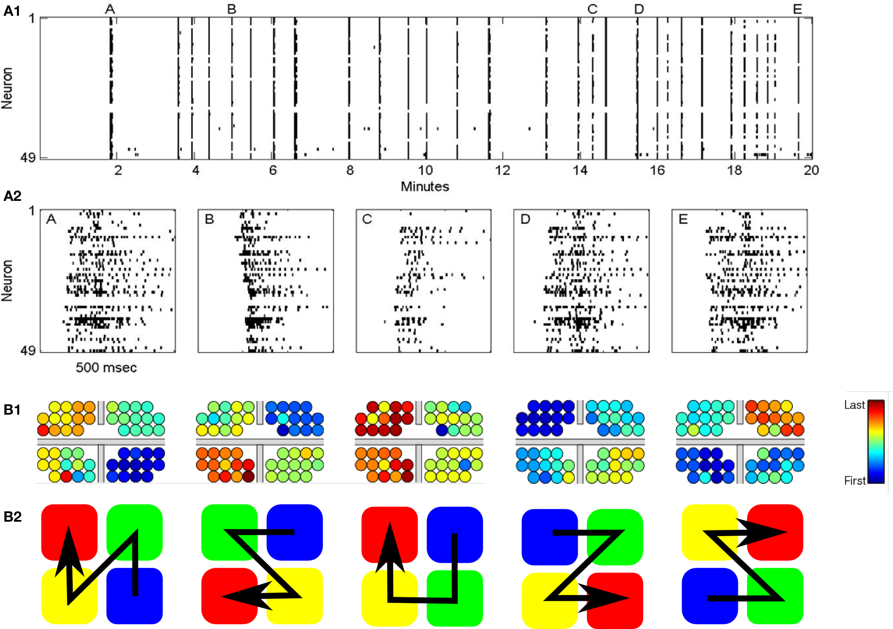
Figure 1. (A1) Typical raster plot of the recorded activity of for coupled neural network. Each line corresponds to the recorded activity from a specific electrodes. Bars indicated neuronal firing. The results show the formation of mutual SBEs. (A2) Zoom in on the raster plot showing five distinct SBEs. (B1) Color code of the order of individual neuron firings within the different APMs from the first firing neuron (blue) to the last (red). Location and size of the electrodes is not in scale. Gray bars mark PDMS lines used to separate between the sub-networks. The order of activity of the four sub-networks follows a wave-like pattern, where the first firing group first activates each of the two nearest clusters. (B2) The activity order of the five leading (most frequent) activity propagation modes (APMs). (A1), (A2), and (B1) are reproduced with permission (Raichman and Ben-Jacob, 2008).

There are a few suggested mechanisms for SBE activity, one of which is based on the hypothesized presence of localized initiation zones. These are characterized by high neuronal density and by recurrent and inhibitory network connections. This hypothesis is anchored on the fact that spontaneous activity is often observed to emanate from localized sources or burst- initiation zones (BIZ), propagating from them to excite large populations of neurons (Raichman and Ben-Jacob, 2008, reviews possible mecahnsimis).

Most of the firing activity is observed within a very short time window at the beginning of the SBE which is then followed by decay over longer period of time (Raichman et al., 2006). Moreover, each neuron in a SBE has its own temporal firing pattern which can greatly vary between different neurons but is usually consistent over days (Raichman and Ben-Jacob, 2008).

The capability of cultured neural networks to spontaneously generate repeating motifs on long time scales (hours) is highly significant for various applications. For example it affords neuronal networks in vitro to maintain long-term memory (Raichman and Ben-Jacob, 2008; Raichman et al., 2009). It was shown that printed (by local chemical stimulation) new activity motifs (activity propagation patterns) can also be maintained by the cultured networks for long times (Baruchi and Ben-Jacob, 2007). The number of motifs and the statistics of their appearance are connected with the architecture (topology, geometry and strengths of synaptic connections) of the network (Volman et al., 2005).

Large networks can generate few different SBEs, each with its own characteristic spatial-temporal pattern of activity propagation across the network (Hulata et al., 2004; Segev et al., 2004). Engineered coupled network, such as the quadruple networks studied here, exhibit different types of mutual SBE, each with its own order of activity propagation between the sub-networks (Baruchi et al., 2008; Raichman and Ben-Jacob, 2008).

SBE Sorting

Dimensionality reduction clustering algorithms (e.g., principle component analysis) are used to identify and sort the different SBE motifs (sometimes referred to as network repertoire). These algorithms enable to simplify the representation of the network activity. In evoked activity experiments where the states of the system are expected due to the controlled stimuli, supervised algorithms can be used (Marom and Shahaf, 2002). However, in the case of spontaneous activity, only un-supervised methods are applicable.

In previous studies, identifications of the distinct SBEs were based on a measure of burst similarity (correlation) metric space. This similarity was defined either by (i) the firing intensity of individual neurons, with disregard of the temporal delays between neurons (Mukai et al., 2003; Madhavan et al., 2006) or (ii) by the time-space correlation between neuronal spike-trains (Segev et al., 2004). The latter approach enables to distinguish between bursts in which the firing profiles of the individual neurons are conserved but with different time delays between the activity of the different neurons. More recently, a delay similarity method was proposed (Baruchi et al., 2008; Raichman and Ben-Jacob, 2008). The method identifies repeating motifs that strictly depend on the delays between initiations of neuronal activity, while disregard the burst intensity and burst duration.

Despite the importance of timing, it has been shown that the information about evoked stimulus position can be retrievable just from the recruitment order, regardless of precise timing (Shahaf et al., 2008). Motivated by these observations we characterize here the different activity propagation modes (APM) of the mutual SBEs in terms of the order of activity propagation between the sub-networks (Figure 1B1).

It is believed that a central property of a complex system is the possible occurrence of coherent large scale collective behaviors with a very rich structure, resulting from the repeated non-linear interactions among its constituents.

Given such a complex system as neuronal network, a first standard attempt in order to quantify and classify the characteristics and the possible different dynamics consists in (i) identifying discrete events, (ii) measuring their features, and (iii) constructing their probability distribution (Sornette, 2007).

In our analysis, these discrete events are the SBE timings and their measured feature is the different APM assigned to each SBE.

Power-Law Scaling

Once identified, we investigated the network repertoire – the statistics of the frequency of appearance of the different APMs. The idea is that similar to the case of other complex systems, the statistics of system level events can provide important clues about the underlying mechanisms that regulate the network activity (Sornette, 2007).

Identification and understanding of such underlying mechanisms that regulate the activity of coupled neural networks can provide important clues on how to regulate, control and change the repertoire of such networks.

We found that half of the networks had algebraic scaling between the frequency of appearance of the leading (more frequent) APMs reminiscence of the Zipf’s power-law scaling of words in natural language. During the 1930s Zipf showed that a power-law distribution described word counts in the English language (Zipf, 1932, 1935). A modern demonstration of this concept on Wikipedia’s corpus has also been shown (Grishchenko, 2006). Research on the origins of the power-law and efforts to observe and validate them in the real world is extremely active in many fields of modern science, and seems to be a ubiquitous statistical feature of complex systems (Bak, 1996; Sornette, 2007).

There is a body of experimental (Beggs and Plenz, 2003, 2004; Petermann et al., 2009) and theoretical work (De Arcangelis et al., 2006; Kinouchi and Copelli, 2006; Levina et al., 2007) on occurrence of power-laws with cutoff in cultured neural networks. In these references the power-law scaling was of the time intervals between events (neuron firing and network bursts). Here, we investigated the statistics of the frequency of appearance of the different APM regardless of their timing.

The Wrestling Model

Toward the interpretation of the observed repertoire, we modeled the interplay between the intrinsic potential to fire of the different BIZ in terms of interacting “clocks” with variable rates. Once one BIZ fires, it stimulates the other BIZs and resets their “clock,” thus disabling their initiation of spontaneous activity. This variable-clock game is an extension of the “boxing arena” model proposed for two coupled networks (Feinerman et al., 2007). Here we extended this work to multiple BIZs and used a Lévy distribution for the clock internal variability and Gaussian distribution for the inter-variability between the clocks. Using maximum likelihood we estimated the model’s parameters and we observed similarity between parameters across cultures with different typical inter-burst-time intervals.

Materials and Methods

Culture and Preprocessing

The experimental protocol of the recordings of the coupled networks’ activity which were analyzed here has been previously presented in details (Raichman and Ben-Jacob, 2008). We used six recorded cultures which are summarized in Table 1 along with their characteristics.

TABLE 1

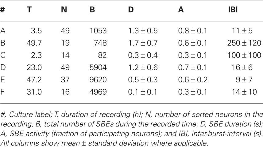
Table 1. Time characteristics of the recorded cultures.

The networks were grown on MEA consisting of 60 round spot recording sites (each with diameter of 30 μm). The spatial organization was specially designed. The electrode array was consisted out of four clusters in the corners of a 1.8 mm × 1.4 mm rectangle. Each cluster was consisted of 13 equally spaced electrodes (250 μm). Other 7 electrodes were located in the regimes between the clusters.

Spike sorting of the extra-cellular recordings was based on wavelet packet decomposition (Hulata et al., 2002). This resulted in a (binary) time series of spike timings with a resolution of milliseconds for each identified neuron.

In order to identify the network bursts we followed the standard procedure of scanning the binary data of the network temporal spike activity in consecutive windows of 2 s, with a 50% overlap. Each window was divided into bins of 200 ms, and each bin was summed up over the number of active neurons. The timing of an SBE was defined as the time bin in which there were a maximum number of active neurons within the 2 s window. We ignored events that had less than 10–50% active neurons, or that were less than 5 s apart from the previously found SBE. Once an SBE was located, we used a pre-trigger and post-trigger of 2 s as the SBE time-support (Chiappalone et al., 2004; Raichman and Ben-Jacob, 2008).

Identifications of the Activity Propagation Modes

As was mentioned earlier, the APM are characterized by the order of activity propagation between the sub-networks (Figure 1B2). With four-coupled networks each APM is described by a permutation of the sequence [1234]. For example, X = [1, 2, 3, 4] means that APM X was such that sub-network “1” fired first, then “2,” “3” and lastly “4.” Therefore, for four sub-networks there are 4! = 24 different possible APMs.

Usually once a sub-network becomes active it does not relax and become active again within the same mutual SBE (representing a finite sub-network refractory period).

Timing the sub-network activity

Three different methods for timing the sub-network activity were tested: (1) average the firing time of first spikes (“first”), (2) center-of-mass of activity profile (“COM”), and (3) max firing rate (“max rate”).

The “first” time is defined as: where N_first is equals to the number of spikes that are considered to be “first” (this number is selected to optimize the measure), and t_k is the time of the kth spike in the ith sub-network.

The motivation to measure only the first spikes, is in line with results showing that spike timing is more accurate in the beginning of the spike-trains, both in spontaneous firing and in bursts generated as a response to electric stimuli. Moreover, it was suggested that bursts propagates as traveling waves where local networks act as the substrate of sequential firing patterns since activity which passes through a given point initiates similar local sequences. (Jimbo and Robinson, 2000; Bonifazi et al., 2005; Luczak et al., 2007; Raichman and Ben-Jacob, 2008; Shahaf et al., 2008).

The number of first spikes N_first introduces a tradeoff between robustness and accuracy. We chose the criterion for choosing N_first to be such that more bursts fall into the same motif, thereby identifying a smaller number of distinct APMs.

The “center-of-mass” time was defined as: where N_tot is the overall number of spikes fired by the sub-network. This method is based on the assumption that different sub-networks fire with similar patterns of firing rate. In this case, averaging the whole firing pattern can produce a fine and robust measure of the sub-network firing pattern. This method assigns larger weight to time periods with higher firing rates in the weighted average. The reason is that such time periods are relatively less noisy (assuming Poisson noise).

The “max rate” time was defined using a histogram: where θ is the Heaviside function and Δt the histogram resolution (1 ms).

The estimated maximum rate time was defined at the center of the histogram maximum: The motivation for this measurement is to order activity of the different sub-networks by the delays of the maximum local activity. The idea is that the first spikes describe the propagation front of the neural signal, but once each sub-network is activated it has its own internal activity propagation.

In the results section we compare between these three timing methods. We then selected the method that yielded the least distinction entropy between the different APMs, following the idea of minimum-entropy data partitioning (Roberts et al., 2001).

Consistency test

In order to test for consistency of our method of identification of the APMs, we compared it with the correlation and delay similarity methods mentioned in the introduction.

The correlation method is based on a binary activity matrix representation of a SBE where N is the number of neurons and T is the number of time bins. The element is if neuron n fired during the time bin t in SBE i = {1…N_SBE} (zero otherwise). First, the activity vector of each neuron is convolved with a normalized Gaussian kernel with width adjusted to the firing rate in order to obtain a smooth rate representation (typically ∼50 ms). Next we define a normalized Pearson’s cross correlation between the bursts couple (i, j) per neuron with time displacement τ:

Finally, a max correlation matrix EC is defined as the maximum (over τ) of the sum (over neurons) of the correlation

This correlation matrix can be interpreted as representation of N_SBE bursts in a N_SBE dimension space. This metric space is then clustered using the dendrogram algorithm tree – an agglomerative hierarchical cluster technique based on distances (Mathworks, 2009). This clustering method allows sorting of the SBEs into different modes, each with its own pattern of correlations between the neuron firings.

The delay similarity method is based on a delay activation matrix B such that is the delay between the first spikes of neuron n and m in the ith SBE. Neurons that did not fire in the particular SBE are assigned a NULL value in the activation matrix. The similarity between bursts is than defined as:

Where θ is the Heaviside function and τ₀ is a threshold which is set to 30 ms following the average spike precision in bursts (Bonifazi et al., 2005). The method detects the center (motive) of SBE clusters with high similarity, by applying a two-stage method that uses a hierarchical clustering algorithm followed by an iterative search for independent cluster centers.

For comparison between the correlation and delay similarity methods with our approach, we used the previous methods’ metric matrix and reordered these matrices in three different fashions: (i) by clustering with respect to the same metric space (e.g., correlation metric reordered according to the correlation space and vice versa), (ii), we repeated the procedure with the alternative metric space (e.g., delay metric reordered based on correlation metric and vice versa), (iii) we reordered the metrics by the APMs that our method identified.

In the result section we show that, while our method is consistent with the other two methods, it is more efficient.

Power-Law Testing and Estimation

To quantify the finite scaling of the frequency of appearance of the different APMs we followed and extended the method of (Goldstein et al., 2004; Clauset et al., 2009). The estimation and significant testing of the power-law (p(k) ∝ k^−β) distribution’s parameter (β) have been extended for the case of the observed finite power-law. This is defined as a finite repertoire of motifs’ (alphabet) distribution which follows the power-law only for k < M where k is the event frequency rank.

We focus only on estimating the power parameter, while M was fixed and chosen such that it differentiated between APMs with frequency higher and lower than that calculated for the limit of uniform frequency of appearance.

The details of the estimation and testing is detailed in the Appendix (see Power-Law Testing and Estimation).

The Wrestling Model

We developed a semi-realistic model which recovers quite efficiently the observed statistical behaviors of the APMs repertoire. This “wrestling” model is an extension for the “boxing arena model” which was proposed for two coupled networks (Feinerman et al., 2007).

The central assumption is that each sub-network has several BIZs and they all “compete” to be the first to initiate a mutual SBE. We assume that each sub-network, had it been isolated from the other sub-networks, have its own innate mean time between SBEs. In other words, each sub-networks a stochastic SBEs generator with its own innate “clock.” However, since the statistics of IBI (inter-bursts-intervals) follows a Lévy distribution (Segev et al., 2002; Ayali et al., 2004), the definition of the generator and the clock have to be done with extra care. In the model used here, we used a stochastic generator that generates a Lévy flight process (Chambers et al., 1976). The generators of the different sub-networks had the same α (slope) and γ (variability) parameters while each sub-network had its own most probable IBI (the δ parameter). The symmetry parameter β_Levy was set to zero (no drift). This difference in δ was generated from a Gaussian distribution with zero mean and STD of and was rolled once before each simulation.

The normalized version of the model has two parameters only: first, the variability variance ratio (η) which is the IBI’s intra-variability variance normalized by the inter-variability variance. Secondly, the Lévy’s distribution power coefficient (α). The details of the model simulation and the procedure of parameter estimation are described in the Appendix (see Model Details and its Parameter Estimation).

Results

Consistency Test

We analyzed the activity of six cultures all having similar structure of four-coupled sub-networks (see Materials and Methods). All of these cultures showed global synchronization marked by the existence of mutual SBEs. First, we show a typical sorting of the different SBEs using the methods of correlation and delay similarity (see Materials and Methods). Then, we compared this similarity/correlation metric matrix when reordered by our new characterization approach.

The new method provides an efficient and clear sorting of SBE into distinct motives of APMs which can be seen as areas of strong intra-group and weak inter-group delay similarity (Figure 2). It is worthwhile noting that although this method achieved a precise classification, it is much less computationally demanding than previous techniques based on metric estimation since the computation of the metric space is not needed.

FIGURE 2

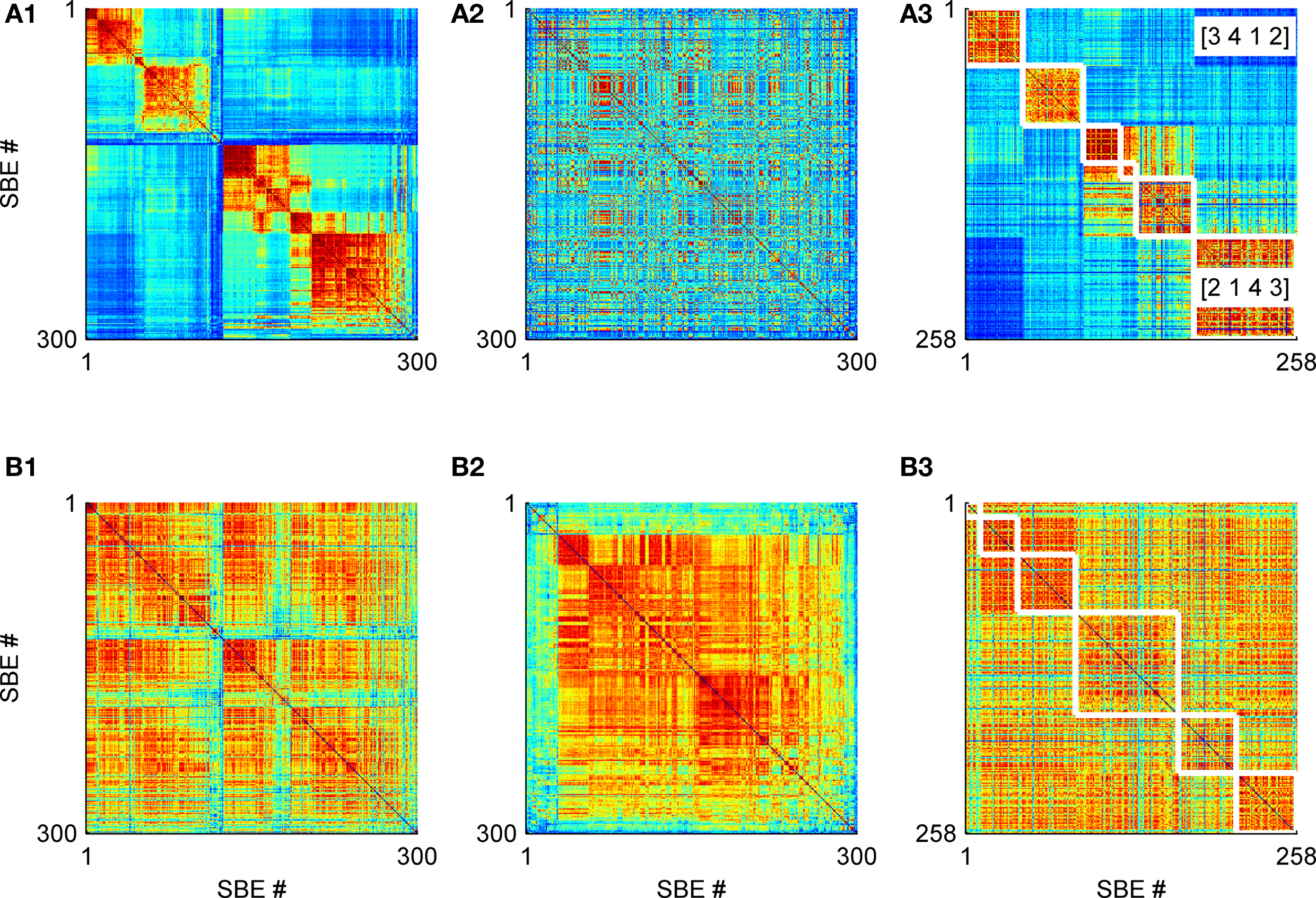
Figure 2. Comparison of delay similarity (row (A)) and correlation (row (B)) metric matrices with culture #A (see Materials and Methods). The x- and y-axis are 300 SBEs indices while the color at each pixel represents the normalized metric value (red-high, blue-low). These metrics were reordered according to three different permutations (1–3 columns): (1) delay similarity, (2) correlation matrix, and (3) our APM method. The latter APMs were bordered (white line) and rearranged (without breaking groups) to fit bets the permutation of the relevant metric (row (A) or (B)). Notice the sequence [3412] and [2143] have opposite activation order and thus have low cross delay similarity metric values.

We found that two APMs with a reverse order of activity propagation, such as the APMs [2, 1, 4, 3] and [3, 4, 1, 2] (Figure 2A3), show low delay similarity. And, two APMs in which the activity starts at the same sub-network show high delay similarity.

Assessment of the Activity Timing Methods

Comparison between the different methods of activity timing revealed that the “first” timing method (based on the firing time of the first few spikes), yields the statistically most significant sorting of the APMs. The statistical significance was assessed by calculating the minimum-entropy data partitioning approach (Roberts et al., 2001). In this approach the entropy of the frequency of appearance of the APMs is calculated (the relative frequency of appearance of each APM is taken as its probability). A distribution with lower entropy corresponds to sorting that is more statistically significant (higher deviation from a uniform distribution).

We found that the best sorting by the “first” timing method is obtained when the first five spikes are taken (N_first = 5) as is shown in Figure 4.

FIGURE 3

Figure 3. Comparison between the significance levels of a power-law model versus an exponential one. Half of the networks showed a significance p-value such that the null hypothesis of a power-law distribution (with cutoff) cannot be declined. On the other hand, only 1/6 of the networks showed similar significance for the exponential model.

FIGURE 4

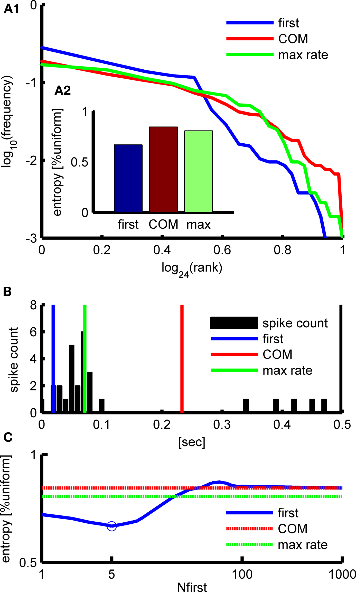
Figure 4. Comparison between the different methods to estimate the APMs’ timing on culture #A (see Materials and Methods). (A1) The frequency of appearance (log) of the frequency of appearance of the APMs using the different methods is similar. (A2) The “first” method shows the closer to power-law like behavior and the entropy. (B) The sub-network activity timing can be measured by averaging the first N_first spikes (blue), by the center-of-mass (COM) of activity (red), or by the maximum firing rate (green) as can be seen plotted on the activity profile histogram (bin size 100 ms). (C) The “first” method entropy is minimized at N_first = 5.

Frequency of Appearance

Half of the networks (three out of six) expressed scaling consistent with a finite power-law with p-value higher than 20% (Figures 5A–C cultures). The three other networks only showed power-law scaling for the leading APMs. Moreover, we compared the power-law with an alternative exponential model. The exponential model was rejected in five out of six networks (Figure 3).

FIGURE 5

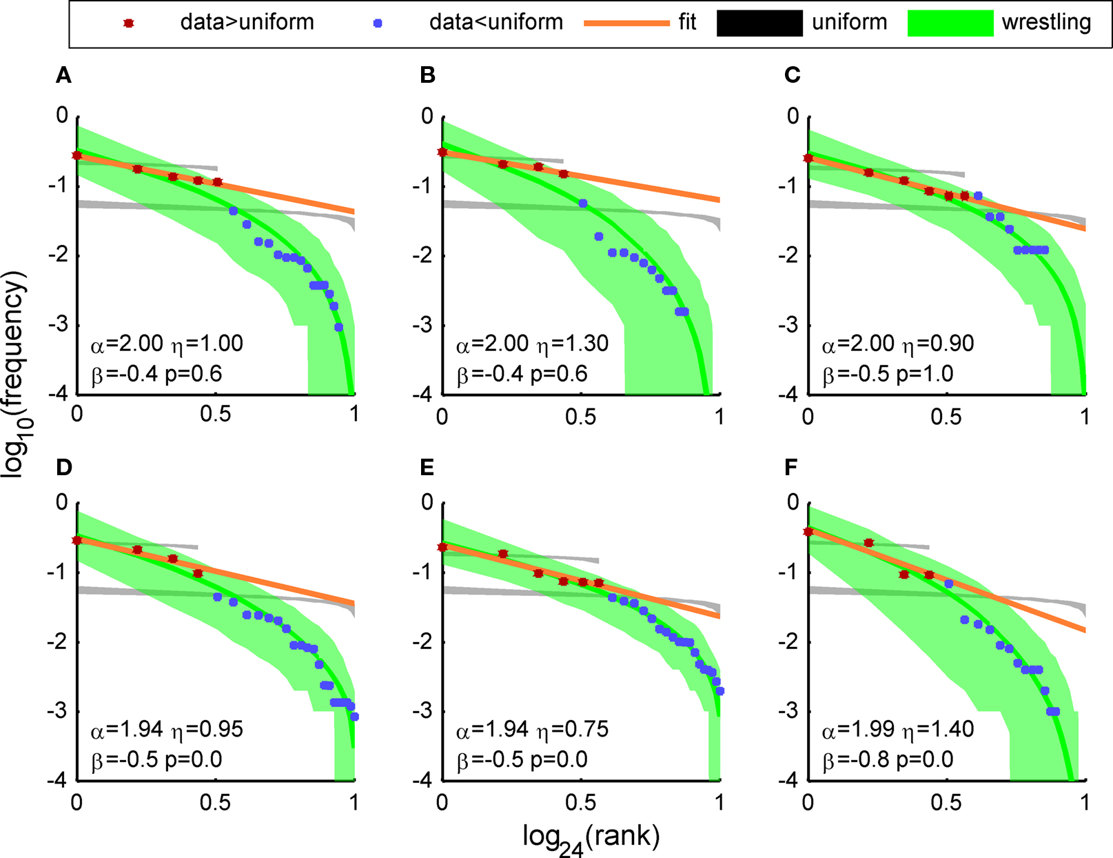
Figure 5. Distributions of the frequency of appearance of the APMs of six different four coupled networks (labeled (A) to (F)). The dots represent the frequency of appearance of the APMs on a log scale, ranked from the most frequent one and down The red dots are the leading (most frequent) APMs – the ones which were more frequent than random (1/24) and blue are the APMs with lower frequency of appearance (including one additional point which was above it). The black patches represent the 1–99% Monte Carlo simulation of a ranking a uniform distribution with alphabet size equal to the maximum number of possible words (24) and to the number of words above uniform (red) (population size = number of culture SBEs and 10,000 repeated simulations). The orange line is the maximum likelihood fit to a power-law model of the points above uniform (red). The Green patches represent the 1–99% Monte Carlo simulation of wrestling model simulation with parameters which were estimated according to maximum likelihood measurement on a grid search (see Materials and Methods). The green line is the mean value of the patch. The number summarize the wrestling arena model simulation parameters (α, η), the power-law estimated slope (β) and the power-law test p-value (p). Notice that also the cultures had very different time properties (e.g., mean IBI lasting from 10 to 250 s; see Materials and Methods) the global distribution parameters are similar and consistent across cultures. Moreover, the maximum likelihood wrestling model fit gives higher values to more frequent events, but nevertheless the model fits nicely also to rare events upto 1 to 1000. In order to emphasize the break of symmetry in the frequency of appearance of the different SAO, we also compared the apparent distribution to a ranking of a uniform distribution. We repeated this first with an alphabet size equal to the maximize number of possible sequence (4! = 24) and secondly with an alphabet size equal to the number of SAO which were more frequent then uniform.

Note that all networks deviated greatly from what would be expected from a uniform distribution of the frequency of appearance (black transparent patches in Figure 5).

Employing the Wrestling Model

The results of the wrestling model simulation are in good agreement with the observed distributions. The level of the agreement indicates that the model may explain some observed features and in particular the four orders of magnitude ratios in the frequency of appearance (see Figure 5 y-axis) and the finite cutoff in the power-law scaling.

Although the different networks had very different time scales and activity, we estimated similar parameters for the different sub-networks.

To avoid confusion we note that there is the set of parameters of the Lévy distribution of the IBI generated by the stochastic generator and the set of parameters of the distribution of the frequency of appearance of the APMs.

The set of parameters for the IBI distributions are defined as: (1) the stability parameter (the slope of the tail of the distribution) – the α parameter of the Lévy distribution. (2) the scaling parameter η, that is equal to the ratio between the variability parameter of the generated IBI sequences (related to the generalization of the STD for Lévy distribution) and the variability (σ_inter) in the mean IBI of the generated IBI sequences of the four different sub-networks is. It is important to note that η equals to 1 for the case that the internal variability of the IBI sequences and the variability between the sub-networks are comparable. The symmetry parameter β_Lévy was set to zero (no drift) and should not be confused with β used here that is the slope of the algebraic (power-law) part of the distribution of the APMs’ frequency of appearance.

Employing the wrestling model, we found that the parameters that fits the observations were: (±SEM) for the Levy distribution and for the power-law slope ( ± SEM). Note that the Lévy slope was almost 2 which is on the edge of Gaussian. We note the similarity across cultures by measuring the coefficient of variance of the model parameters: CV(α, β, γ) = (0.01, 0.28, 0.24). We also note that, five out of six cultures passed a leave-one-out multi-variant ANOVA test with 5% threshold with the null hypothesis being the same parameters mean.

An additional important observation is related to the value of the inter-burst-time interval (IBI) which preceded the appearance of each APM. The wrestling model predicts that the distribution of the observed bursts IBIs would be of the same order of magnitude for the different sub-networks in agreement with the experimental observations.

In other words, the mean IBI of a specific BIZ conditioned of it being the shortest one in the current round is smaller than the aggregated IBI mean and is comparable to the most frequent BIZ’s IBI:

We compare the simulation result to the real data by treating each APM as it was generated by different IBI and in both the “winning” IBIs is relatively flat (Figure 6).

FIGURE 6

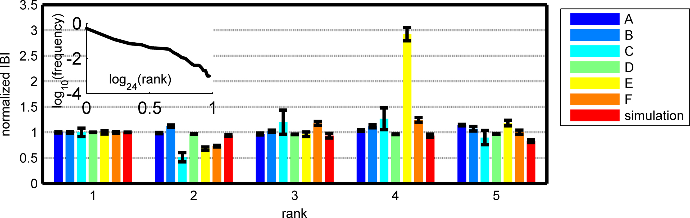
Figure 6. Mean IBI just before one of the five most frequent (highest rank) APMs of six different networks and a simulation of the “wrestling arena. ” We normalized these IBI according the mean IBI of the most frequent APMs (thus the most frequent mean is “1”) (errors are SEM). It seems that the IBI before each APM is the same for the different leading APMs despite the high variability of the IBIs. The wrestling model predicts this (typical simulation α = 1.9, η = 1, N = 1000). The model predicts that if a slower BIZ wins over the most frequent APM its IBI is shorter than usual and of the same order of magnitude as the most frequent APM (or smaller). Note that the wrestling simulation can produce a finite power-law like behavior (not in all runs) with a cutoff similar to the observed data.

Discussion and Summary

We showed that four-coupled cultured networks exhibit mutual SBEs with a reach repertoire of APM, each with a distinct order of activity propagation between the sub-networks. Investigations of the frequency of appearance of the APMS revealed power-law scaling between the several leading (most frequent) ones. In complex systems, power-law scaling can be a manifestation of hierarchy and robustness (Sornette, 2007). The non-uniform nature of Finite power-law suggests some kind of control mechanism that prevents a winner-takes-all scenario by the most active sub-network (so it does not generate almost all the mutual SBE).

We introduced a “wrestling model” to account for the observations. Simulations of the model to fit with the observations revealed that the scaling parameter η has to be close to 1. This result indicates that the intrinsic variability in the IBI sequences generated by the sub-networks is regulated to fit the variability in the mean IBI between the different sub-networks.

This result suggests that there must be some unknown mechanism which can co-regulate the local intra-variability and the global inter-variability to be comparable.

One possible mechanism might be related to the propagation of calcium waves in the astrocytes. It has been proposed that astrocyte calcium waves may constitute a long-range signaling system within the brain (Cornell-Bell et al., 1990).

The calcium waves can be regulated by the rate of activity of the different sub-networks and in turn regulates the effective synaptic strengths. Since they have a long time scales and can propagate over long distances, the calcium waves might provide a mechanism that couples the intrinsic scaling of IBI and the global variability between the different sub-networks. The possible role of calcium wave can be tested experimentally by testing the effect of regulations of the astrocyte calcium wave’s dynamics on the frequency of appearance of the APMs.

Finally we would like to note that the similarity in the model’s parameters across cultures might suggests that these are invariants of the culture network.

Appendix

Power-Law Testing and Estimation

To quantify the finite scaling of the frequency of appearance of the different APMs we followed and extended the method of (Goldstein et al., 2004; Clauset et al., 2009). The estimation and significant testing of the power-law (p(k) ∝ k^−β) distribution’s parameter (β) have been extended for the case of the observed finite power-law. This is defined as a finite repertoire of motifs’ (alphabet) distribution which follows the power-law only for k < M where k is the event frequency rank. We focus only on estimating the power parameter, while M was fixed and chosen such that it differentiated between APMs with frequency higher and lower than that calculated for the limit of uniform frequency of appearance.

Finite power-law estimation

We estimated the power-law only on a subset of the distribution at k < M. The justification for this approach is as follows: if the subset accumulates q fraction of the whole distribution P₀, the subset distribution P is related to it as P = qP₀. Since maximum likelihood estimation maximizes P and since q is independent on the distribution parameters (β), it can be omitted and P can be treated as if it was the real distribution.

Assuming that the one sample distribution is defined as:

where is the partition function for the case of M discrete values and the exponent β. Note that this is not the real partition function and it does not normalize the whole distribution rather only the power-law subset part.

If the measurements are statistically independent, the log likelihood (λ) of β with N observations can be written as To find its minimum, we differentiate with respect to the parameter and get the ML estimator:

where we mark the partition function derivation as

Thus we get the implicit expression for the estimated power

which can be solved numerically for every observation set and fixed M.

Power-law testing

Observing an approximately straight line on a log-log plot is a necessary but not sufficient condition to indicate power-law scaling (Clauset et al., 2009). Thus, we tested the hypothesis of power-law distribution in a statistically significant manner using goodness-of-fit test based on Kolmogorov–Smirnov (KS) statistic test (Goldstein et al., 2004). A significant p-value for this test (typical more than 0.05) means that the power-law null hypothesis cannot be rejected which means that the data is compatible with the null hypothesis.

To avoid estimation bias, we used a Monte Carlo calibration process in which we drew a large number (n ∼ 10³) of synthetic data sets from different power-laws distributions with uniform random slope α in the range [0, 1] (α ∼ U(0, 1)) of discrete alphabet size M ∈ [3, 24]. Then we fitted each one individually to the power-law model (see previous subsection) and calculated the KS statistic for each one relative to its own best-fit model. We then measured the test’s p-value by estimating the fraction of trials which had a KS value larger than the observed one.

To summarize, in order to test the hypothesis that the observed data set is drawn from a power-law distribution one should: (1) Determine the best fit of the power-law to the data by estimating the scaling parameter β using the ML method, (2) Calculate the KS statistics for the goodness-of-fit of the best-fit power-law to the data, (3) generate a large number of synthetic data sets. Fit each according to the ML method, and calculate the KS statistic for each fit, (4) calculate the p-value as the fraction of the KS statistics for the synthetic data sets whose value exceeds the KS statistic for the real data, (5) If the p-value is sufficiently small, the power-law distribution can be ruled out (Clauset et al., 2009).

An analysis of the expected worst-case performance of the method produced a rule of thumb for determine the number of trials (n): if the p-values is to be accurate to within about ε of the true value, then at least (2ε)⁻² synthetic data sets should be generated (Clauset et al., 2009). If, for example, the p-value is accurate to about two decimal points, ε = 0.01 should be chosen, which implies a generation of about 2500 samples minimum. In our test, we used 10,000.

Model Details and Its Parameter Estimation

At each round (r = [1, N_r], N_r = 1000) the ith BIZ produces a random IBI according to the sum of its own mean IBI μ_i ∝ N(0, σ_inter) and its centered Lévy distribution realization such that At each round the winning BIZ (W^r) is the one with the shortest IBI: The histogram of winning BIZs is then sorted (ranked) and normalized where δ(i, j) being the Kronecker’s delta. The probability distribution of the different ranks is thus simply

We estimated the model parameters by a grid search (α = [1:0.01:2], η = [0.5:0.05:2]). For each couple of parameters, we estimated the probability distribution of each rank Then we computed the log likelihood by modeling the observed frequency of rank as multinomial distribution. We found which maximize the log likelihood Γ using the relation For the ML estimated parameters’ values we computed the 98% (1–99%) confidence interval of the frequency of appearance for each rank (from the same Monte Carlo simulation).

Obviously, when the scaling parameter η is large we expect only one BIZ to win (“winner-takes-it-all” scenario), thus producing a delta function in the ranked SAO distribution. However, if it is small, it would create a uniform distribution since all BIZ are equally likely to “win.” We claim that only variability ratio of the order of one (η ∼ 1) can explain the observed SAO distribution which is neither uniform nor exclusive.

We note that η is somehow problematic as for α lower than 2, the variance of the Lévy’s distribution diverges. Therefore, we used the empiric variance and normalized it according to

Conflict of Interest Statement

The authors declare that the research was conducted in the absence of any commercial or financial relationships that could be construed as a potential conflict of interest.

Acknowledgments

We are thankful to Liel Rubinsky and Mark Shein. One of us HS thanks Prof. Hagit Messer-Yaron for partial support during part of this research. This research has been supported in part by the Tauber Family Foundation and the Maguy-Glass Chair in Physics of Complex Systems at Tel Aviv University.

References

Ayali, A., Fuchs, E., Zilberstein, Y., Robinson, A., Shefi, O., Hulata, E., Baruchi, I., and Ben-Jacob, E. (2004). Contextual regularity and complexity of neuronal activity: from stand-alone cultures to task-performing animals. Complexity 9, 25–32.

CrossRef Full Text

Bak, P. (1996). How Nature Works: The Science of Self-Organised Criticality. New York, NY: Copernicus Press.

Baruchi, I., and Ben-Jacob, E. (2007). Towards neuro-memory-chip: imprinting multiple memories in cultured neural networks. Phys. Rev. E, Stat. Nonlin. Soft Matter Phys. 75, 509011–509014.

CrossRef Full Text

Baruchi, I., Volman, V., Raichman, N., Shein, M., and Ben-Jacob, E. (2008). The emergence and properties of mutual synchronization in in vitro coupled cortical networks. Eur. J. Neurosci. 28, 1825–1835.

Pubmed Abstract | Pubmed Full Text | CrossRef Full Text

Beggs, J. M., and Plenz, D. (2003). Neuronal avalanches in neocortical circuits. J. Neurosci. 23, 11167–11177.

Pubmed Abstract | Pubmed Full Text

Beggs, J. M., and Plenz, D. (2004). Neuronal avalanches are diverse and precise activity patterns that are stable for many hours in cortical slice cultures. J. Neurosci. 24, 5216–5229.

Pubmed Abstract | Pubmed Full Text | CrossRef Full Text

Bonifazi, P., Ruaro, E., and Torre, V. (2005). Statistical properties of information processing in neuronal networks. Eur. J. Neurosci. 22, 2953–2964.

Pubmed Abstract | Pubmed Full Text | CrossRef Full Text

Chambers, J. M., Mallows, C. L., and Stuck, B. W. (1976). A method for simulating stable random variables. J. Am. Stat. Assoc. 71, 340–344.

CrossRef Full Text

Chiappalone, M., Novellino, A., Vato, A., Martinoia, S., Vajda, I., and van Pelt, J. (2004). Analysis of the Bursting Behavior in Developing Neural Networks. 2nd International Symposium on Measurement, Analysis and Modeling of Human Functions, Genova.

Chiappalone, M., Vato, A., Berdindini, L., Koudelka-Hep, M., and Martinoia, S. (2007). Network dynamics and synchronous activity in cultured cortical neurons. Int. J. Neural. Syst. 17, 87–103.

Pubmed Abstract | Pubmed Full Text | CrossRef Full Text

Clauset, A., Shalizi, C. R., and Newman, M. E. J. (2009). Power-law distributions in empirical data. SIAM Rev. 51, 661–703.

CrossRef Full Text

Cornell-Bell, A. H., Finkbeiner, S. M., Cooper, M. S., and Smith, S. J. (1990). Glutamate induces calcium waves in cultured astrocytes: long-range glial signaling. Science 247, 470–473.

Pubmed Abstract | Pubmed Full Text | CrossRef Full Text

De Arcangelis, L., Godano, C., Lippiello, E., and Nicodemi, M. (2006). Universality in solar flare and earthquake occurrence. Phys. Rev. Lett. 96, 051102–051105.

Pubmed Abstract | Pubmed Full Text | CrossRef Full Text

Feinerman, O., Segal, M., and Moses, E. (2007). Identification and dynamics of spontaneous burst initiation zones in unidimensional neuronal cultures. J. Neurophysiol. 97, 2937–2948.

Pubmed Abstract | Pubmed Full Text | CrossRef Full Text

Goldstein, M. L., Morris, S. A., and Yen, G. G. (2004). Problems with fitting to the power-law distribution. Eur. Phys. J. B 41, 255–258.

CrossRef Full Text

Grishchenko, V. (2006). Wikipeida/Zipf’s_law. License, GNU Lesser General Public. Available at http://en.wikipedia.org/wiki/Zipf%27s_law.

Hulata, E., Baruchi, I., Segev, R., Shapira, Y., and Ben-Jacob, E. (2004). Self-regulated complexity in cultured neuronal networks. Phys. Rev. Lett. 92, 198181–198104.

CrossRef Full Text

Hulata, E., Segev, R., and Ben-Jacob, E. (2002). A method for spike sorting and detection based on wavelet packets and Shannon’s mutual information. J. Neurosci. Methods 117, 1–12.

Pubmed Abstract | Pubmed Full Text | CrossRef Full Text

Jimbo, Y., and Robinson, H. P. C. (2000). Propagation of spontaneous synchronized activity in cortical slice cultures recorded by planer electrode arrays. Bioelectrochemistry 51, 107–115.

Pubmed Abstract | Pubmed Full Text | CrossRef Full Text

Kinouchi, O., and Copelli, M. (2006). Optimal dynamical range of excitable networks at criticality. Nat. Phys. 2, 348–351.

CrossRef Full Text

Koch, C., and Laurent, G. (1999). Complexity and the nervous system. Science 284, 96–98.

Pubmed Abstract | Pubmed Full Text | CrossRef Full Text

Levina, A., Herrmann, J. M., and Geisel, T. (2007). Dynamical synapses causing self-organized criticality in neural networks. Nat. Phys. 3, 857–860.

CrossRef Full Text

Luczak, A., Bartho, P., Marguet, S. L., Buzsaki, G., and Harris, K. D. (2007). Sequential structure of neocortical spontaneous activity in vivo. Proc. Natl. Acad. Sci. U.S.A. 104, 347–352.

Pubmed Abstract | Pubmed Full Text | CrossRef Full Text

Madhavan, R., Chao, Z. C., and Potter, S. M. (2006). Spontaneous Bursts are Better Indicators of Tetanus-Induced Plasticity than Responses to Probe Stimuli. Neural Engineering, 2005. Conference Proceedings. 2nd International IEEE EMBS Conference, Arlington, VA, V–VIII.

Marom, S., and Shahaf, G. (2002). Development, learning and memory in large random networks of cortical neurons: lessons beyond anatomy. Q. Rev. Biophys. 35, 63–87.

Pubmed Abstract | Pubmed Full Text | CrossRef Full Text

Mathworks. (2009). MATLAB Statistics Toolbox. Natick, MA: Mathworks.

Mukai, Y., Shina, T., and Jimbo, Y. (2003). Continuous monitoring of developmental activity changes in cultured cortical networks. Electr. Eng. Jpn. 145, 28–37.

CrossRef Full Text

Petermann, T., Thiagarajan, T. C., Lebedev, M. A., Nicolelis, M. A. L., and Chialvo, D. R. (2009). Spontaneous cortical activity in awake monkeys composed of neuronal avalanches. Proc. Naatl. Acad. Sci. U.S.A. 106, 15921–15926.

CrossRef Full Text

Potter, S. M. (2001). Distributed processing in cultured neuronal networks. Prog. Brain Res. 130, 49–62.

Pubmed Abstract | Pubmed Full Text | CrossRef Full Text

Raichman, N., and Ben-Jacob, E. (2008). Identifying repeating motifs in the activation of synchronized bursts in cultured neuronal networks. J. Neurosci. Methods 170, 96–110.

Pubmed Abstract | Pubmed Full Text | CrossRef Full Text

Raichman, N., Rubinsky, L., Shein, M., Baruchi I., Volman V., and Ben-Jacob, E. (2009). “Cultured neuronal networks express complex patterns of activity and morphological memory,” in Handbook of Biological Networks, eds S. Boccaletti, V. Latora, and Y. Moreno Singapore: (World Scientific), 257–278.

Raichman, N., Volman, V., and Ben-Jacob, E. (2006). Collective plasticity and individual stability in cultured neuronal networks. Neurocomputing 69, 1150–1154.

CrossRef Full Text

Roberts, S. J., Holmes, C., and Denison, D. (2001). Minimum-entropy data partitioning using reversible jump markov chain monte carlo. IEEE Trans. Pattern Anal. Mach. Intell. 23, 909–914.

CrossRef Full Text

Segev, R., Baruchi, I., Hulata, E., and Ben-Jacob, E. (2004). Hidden neuronal correlations in cultured networks. Phys. Rev. Lett. 92, 118102.

Pubmed Abstract | Pubmed Full Text | CrossRef Full Text

Segev, R., Benveniste, M., Hulata, E., Cohen, N., Palevski, A., Kapon, E., Shapira, Y., and Ben-Jacob, E. (2002). Long term behavior of lithographically prepared in vitro neuronal networks. Phys. Rev. Lett. 88, 1181021–1181024.

CrossRef Full Text

Shahaf, G., Eytan, D., Gal, A., Kermany, E., Lyakhov, V., Zrenner, C., and Marom, S. (2008). Order-based representation in random networks of cortical neurons. PLoS Comput. Biol. 4, e1000228. doi: 10.1371/journal.pcbi.1000228.

Pubmed Abstract | Pubmed Full Text | CrossRef Full Text

Sornette, D. (2007). Probability Distributions in Complex Systems. arXiv:0707.2194, ARXIV.

Volman, V., Baruch, I., and Ben-Jacob, E. (2005). Manifestation of function-follow-form in cultured neuronal networks. Phys. Biol. 2, 98–110.

Pubmed Abstract | Pubmed Full Text | CrossRef Full Text

Zipf, G. (1932). Selective Studies and the Principle of Relative Frequency in Language. Cambridge, MA: MIT Press.

Zipf, G. (1935). Psycho-Biology of Languages. Boston, MA: Houghton-Mifflin (1934), MIT Press (1965).