Emergence of modular structure in a large-scale brain network with interactions between dynamics and connectivity

Introduction

Anatomical and functional networks in the brain display a complex architecture, which is supposed to underlie optimal information processing. In particular, the structure of these networks may explain the balance between segregation and integration of functions in the brain (Sporns et al., 2004). Progress in modern network theory, spurred by the discovery of small-world and scale-free networks, has provided us with the suitable concepts and analytic tools to characterize the complex structure of brain networks, and to relate their topological organization to their function (Boccaletti et al., 2006). Like a wide range of other natural and technological networks, brain networks are characterized by short path lengths, high clustering, heavy tailed degree distributions, hubs, degree correlations, and a modular architecture. These topological characteristics have been demonstrated in the central nervous system of various organisms, ranging from C. elegans to humans (Reijneveld et al., 2007; Stam and Reijneveld, 2007; Bullmore and Sporns, 2009). Similar patterns are seen in structural as well as functional networks. Complex network features have been described at the level of interconnected neurons (Yu et al., 2008; Bonifazi et al., 2009), as well as at the macroscopic level of interconnected brain regions (Hagmann et al., 2008). Moreover, there is evidence that various features of complex brain networks are relevant for brain function, in particular higher level capacities such as intelligence (Li et al., 2009; Van den Heuvel et al., 2009). It is still unclear though how this complex topology of brain systems arises, and which factors play an important role in determining the final topology.

An important distinction between complex and complicated systems is that complex systems derive their final structure from a process of self-organization rather than from a pre-defined blueprint. The complex structure of adult brain networks is very likely an emergent feature of growing and developing neural networks, that shape their structure under influence of trophic, geometric and activity dependent factors. Most likely, some of these factors that operate during development are under genetic control, since topological features of adult brain networks have a strong heritability (Smit et al., 2008, 2010). However, any genes involved can only guide general principles of network growth; we have vastly more synapses in our brain than we have genes to specify them.

One way to study the mechanisms involved in the emergence of complex brain networks is to use model systems. Graph theoretical analysis of neural networks cultured in multi-electrode arrays has shown that such networks evolve from a random initial topology to a typical small-world network characterized by short path lengths and high clustering (Bettencourt et al., 2007; Srinivas et al., 2007). In vitro studies confirm the self-organizing properties of developing neural networks, but do not allow direct identification of the causal mechanisms. In a computational model of interconnected units consisting of logistic functions, activity dependent rewiring such that synchronous units become increasingly connected, results in an evolution from a random topology toward a small-world network with modular features (van den Berg and van Leeuwen, 2004; Rubinov et al., 2009b). In this model, chaotic dynamics of the individual units and weak connectivity were essential in giving rise to a modular functional organization that subsequently drove the structure of the underlying network. These results have been replicated using Hindmarsh Rose neurons instead of logistic functions as network nodes (Zhou et al., 2007). Work by Kaiser and Hilgetag (2004, 2007) has shown that distance effects are also important in shaping the topology of the growing networks. Other studies have used networks of model neurons with different types of activity dependent plasticity such as Hebbian learning, spike timing dependent plasticity (STDP) and synaptic scaling to study the interactions between network dynamics and structural network evolution (Song et al., 2000; Jun and Jin, 2007; Levina et al., 2007; Siri et al., 2007; Fuchs et al., 2009). In general, these model studies show that activity dependent modulation of synaptic strength induces an emergent feature in the complex network. In addition, under suitable conditions the resulting networks may also display critical, scale-free dynamics (Levina et al., 2007). Such critical dynamics have been associated with optimal information processing and learning (Kinouchi and Copelli, 2007; de Arcangelis and Herrmann, 2010).

Most of the models discussed above involve some kind of circular causality between dynamic processes on the network, and the slow modulation of the networks connectivity or adjacency matrix. Dynamic processes change the connectivity, while the connectivity constrains the dynamics. The fundamental principles of such processes have been addressed only recently (Aoki and Aoyagi, 2009; Grindrod and Higham, 2009). In addition, in vitro or in silico models of neural networks cannot be directly translated to structural and functional networks as studied with electroencephalography (EEG), magnetoencephalography (MEG), and functional/structural magnetic resonance imaging (MRI) in humans. It has been shown that macroscopic models of brain networks may explain the topology of functional networks at various time scales (Honey et al., 2007, 2009). In addition, macroscopic models have been used to predict the consequences of various types of lesions on brain networks (Honey and Sporns, 2008; Alstott et al., 2009). Systematically varying the topology of the structural network will change the features of the corresponding functional network (Ponten et al., 2010). Thus, the macroscopic level is crucial to connect modeling work to direct empirical observations in humans, but it is currently unclear how network evolution and plasticity, as well as recovery from damage, should be modeled at this level.

In the present study, we investigate a macroscopic model of complex brain networks consisting of 32 or 64 interconnected neural masses (Ponten et al., 2010). Each neural mass represents a large population of interconnected excitatory and inhibitory neurons, generating an average voltage that reflects the EEG or MEG signal generated by this population. We simulate neural development and plasticity by two processes: (i) growth dependent plasticity (GDP), a homeostatic mechanism where neural masses grow new connections, or delete old connections, in order to maintain a connection pattern that decays exponentially with distance, as has been observed in real neural networks (Kaiser et al., 2009); (ii) synchronization dependent plasticity (SDP) where connections between neural masses are strengthened if they fire synchronously, and weakened if they do not. Starting from initially unconnected networks we investigate how an interaction of SDP and GDP shapes the final network structure, in particular the presence of modules. Finally, we study the time dependent response of the evolved networks to acute lesions.

Materials and Methods

Description of the Neural Mass Model

We used a model of interconnected neural masses, where each neural mass represents a large population of connected excitatory and inhibitory neurons generating an EEG or MEG like signal. The model was described in Ponten et al. (2010). The basic unit of the model is a neural mass model (NMM) of the alpha rhythm (Lopes da Silva et al., 1974; Zetterberg et al., 1978). The same model was used in a previous study on bifurcation phenomena of the alpha rhythm (Stam et al., 1999). As previously described, this model considers the average activity in relatively large groups of interacting excitatory and inhibitory neurons. Spatial effects are ignored in this model; we will introduce spatial effects later by coupling several NMMs together. The excitatory and inhibitory populations of each NMM are characterized by their average membrane potentials V_e(t) and V_i(t), and by their pulse densities, i.e., the proportion of cells firing per unit time E(t) and I(t). Static non-linear functions S_E(x) and S_I(x) relate the potentials V_e(t) and V_i(t) to the corresponding pulse densities E(t) and I(t). The excitatory post-synaptic potential (EPSP) and inhibitory post-synaptic potential (IPSP) are modeled by the impulse responses h_e(t) and h_i(t). The constants C₁ and C₂ describe the coupling from excitatory to inhibitory and from inhibitory to excitatory populations respectively. P(t) is the pulse density of an input signal to the excitatory population. Following Zetterberg et al. (1978) the following impulse responses were used:

For h_e(t) the parameter values were: A = 1.6 mV, a = 55 s⁻¹, b = 605 s⁻¹. For h_i(t) the parameter values were: A = 32 mV, a = 27.5 s⁻¹, b = 55 s⁻¹. The sigmoid function relating the average membrane potential, V_m, to the impulse density was also taken from Zetterberg et al. (1978):

Here the parameter values used were: q = 0.34 mV⁻¹, V_d = 7 mV, g = 25 s⁻¹. For the coupling constants we used C₁ = 32 and C₂ = 3 (Lopes da Silva et al., 1974). A schematic representation is shown in Figure 1A. All model parameters are summarized in Table 1. The impulse response and sigmoid functions are shown in Figure 1C.

FIGURE 1

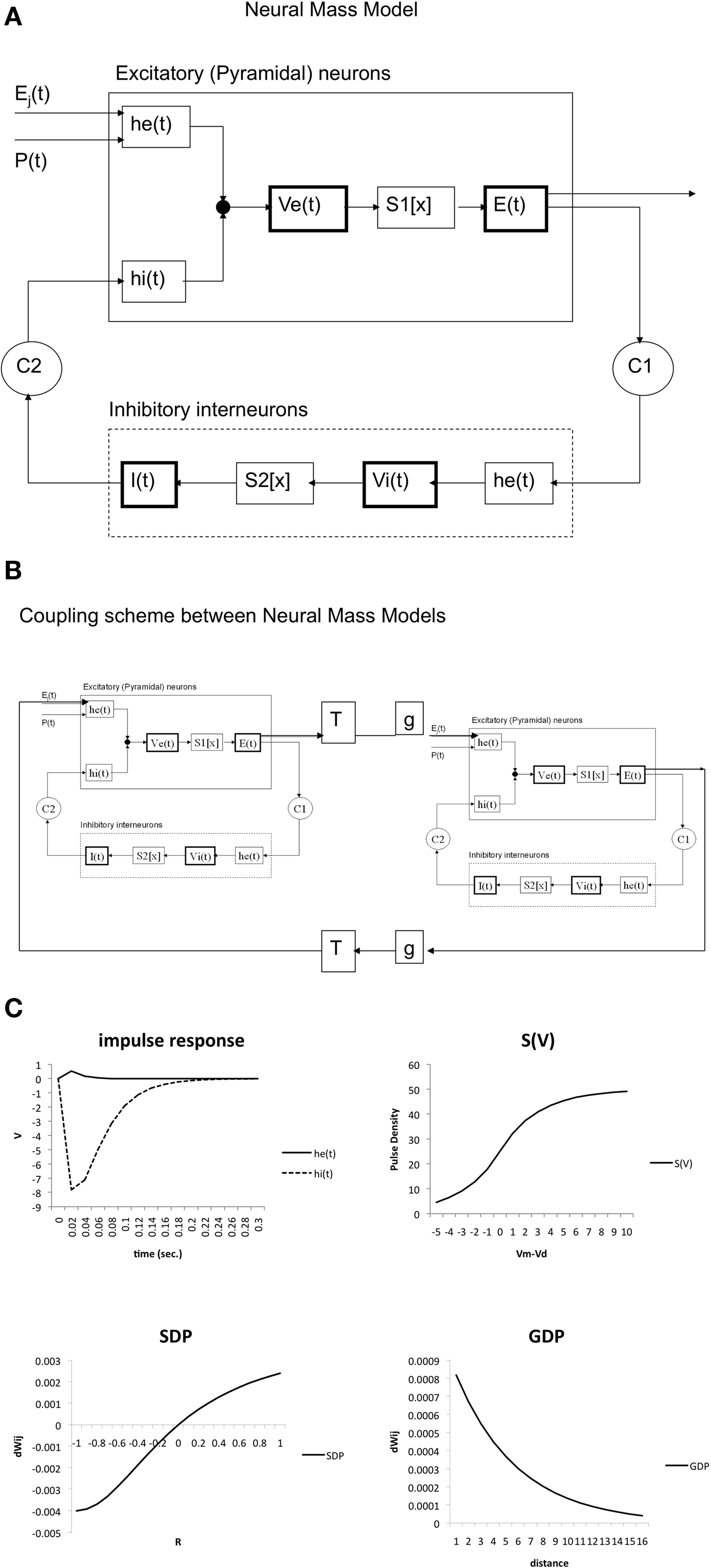
Figure 1. (A) Schematic presentation of single neural mass model. The upper rectangle represents a mass of excitatory neurons, the lower rectangle a mass of inhibitory neurons. The state of each mass is modeled by an average membrane potential [V_e(t) and V_i(t)] and a pulse density [E(t) and I(t)]. Membrane potentials are converted to pulse densities by sigmoid functions S₁[x] and S₂[x]. Pulse densities are converted to membrane potentials by impulse responses h_e(t) and h_i(t). C₁ and C₂ are coupling strengths between the two populations. P(t) and E_j(t) are pulse densities coming from thalamic sources or other cortical areas respectively. (B) Coupling of two neural mass models. Two masses are coupled via excitatory connections. These are characterized by a fixed delay T and a strength g. (C) Essential functions of the model. The upper left panel shows the excitatory [h_e(t)] and inhibitory [h_i(t)] impulse responses of Eq. 1. The upper right shows the sigmoid function relating average membrane potential to spike density (Eq. 2). At the lower left the growth dependent plasticity (GDP) is shown (Eq. 4). At the lower right the synchronization dependent plasticity (SDP) is shown (Eq. 3).

TABLE 1

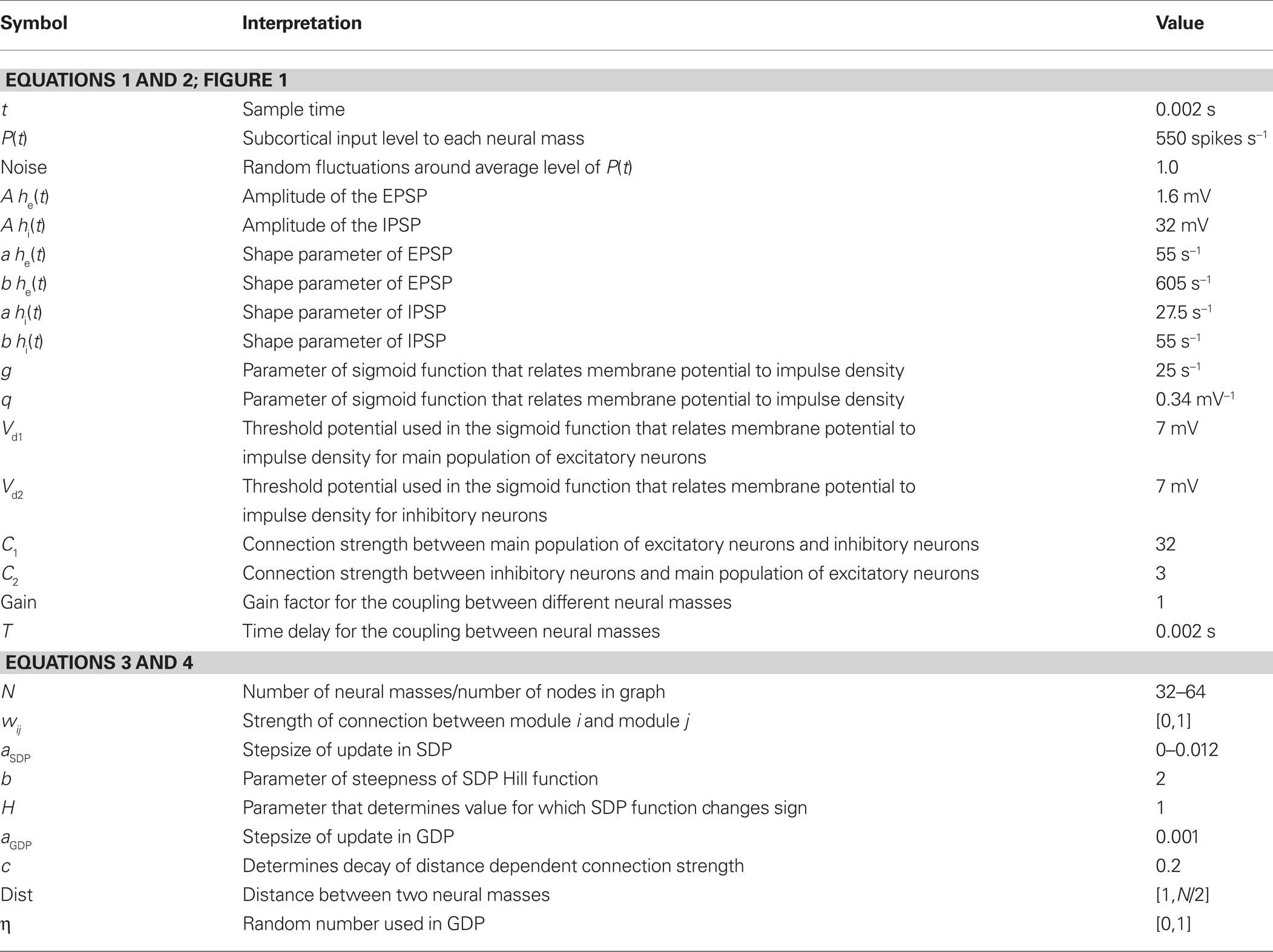
Table 1. Overview of model parameters.

The final model consisted of several of the NMMs as described above, which were coupled together. Coupling between two NMMs, if present, was always reciprocal, and excitatory. The output E(t) of the main excitatory neurons of one NMM was used as the input for the impulse response h_e(t) of the excitatory neurons of the second NMM; the output E(t) of the second module was coupled to the impulse response h_e(t) of the excitatory neurons of the first NMM. Following Ursino et al. (2007) we used a time delay (T × sample time, with n an integer, 0 < T < 21) and a gain factor. In the present study, n and gain were set to 1 for all connections. A schematic illustration of the coupling between two NMMs is shown in Figure 1B.

In the present study, the model was programmed in Java and implemented in the program BrainWave (version 0.8.47) written by C. J. Stam (Stam et al., 1999). The Java code was based on the Pascal source code described by Schuuring (1988). For the present study the model was extended in order to be able to deal with activity dependent evolution of connection strength between multiple coupled NMMs. The impulse responses, h(t), were implemented as a convolution in the discrete time domain in a similar way as in the Pascal program.

The average membrane potential of the excitatory neurons V_e(t) of each of the NMMs separately was the multichannel output. The sample frequency was 500 Hz. In the present study each run consisted of 9096 (18.19 s). The adjacency matrix at the end of each run was subjected to topographical analysis. Table 1 gives an overview of model parameters and initial settings. These parameters go back to large number of studies with this lumped model, and ultimately to the original model of Lopes da Silva et al. (1974). For the new parameters in the present study, to be discussed below, we choose to keep the parameters of GDP constant (such that they would result in a reasonable outgrowth of connections), and systematically vary the SDP stepsize, as shown in Figures 5 and 6.

Modeling of Network Plasticity and the Interaction Between Dynamics and Connectivity

In our previous study the strength of connections between neural masses was always symmetrical, and the same strength was used for all connections (Ponten et al., 2010). In the present study we assign a weight w_ij ∈ [0,1] to the connections between two neural masses i and j, where w_ij = w_ji. We update the connection weights w_ij once every 100 time steps using two processes.

The first process for updating the connection weights is GDP. This process reflects that neural masses will increase or decrease their connection strengths to other neural masses when they deviate from a reference value, determined by a distance dependent decay. GDP is also applied once every 100 time steps, directly after SDP. In contrast to SDP, GDP is applied to all connections, even those with w_ij = 0. The connection weight update is given by:

Here, a_GDP is the GDP step size, which is chosen as 0.001. Θ is a modified Heaviside function, with Θ(x) = 1 if x < 0, and Θ(x) = −1 if x > 0. The term w_th = e^−cDist is the reference value to which the weight w_ij is compared, with c determining the decay rate of the exponential. We chose c = 0.2. Dist is the distance between the neural masses i and j, an integer taken from the interval [1,N/2], with N the number of neural masses and circular boundary conditions. The noise parameter η is a real number taken randomly from the interval [0,1]. The GDP and SDP functions are shown in Figure 1C.

The second is SDP. With SDP the weights of all connections w_ij > 0 are updated with a small step given by a Hill function:

Here a_SDP is referred to as the SDP step size and r is the correlation between the pulse densities E(t) of two neural masses i and j, computed over the preceding 20 time steps, +1. The range of r is [0,2]. The exponent b, which determines the steepness of the Hill function, is chosen as 2. H determines where the function crosses the line Δw_ij = 0 and is chosen as 1. With this function, Δw_ij is bounded between −0.5 a_SDP and 0.3 a_SDP. SDP reflects how the connection strength between two neural masses will increase if they show correlated firing, and will decrease if they do not. If the update results in w_ij < 0, w_ij is set to 0, and the connection is considered to be lost. If the update results in w_ij > 1, it is reset to w_ij = 1.

Weighted Graph Analysis

The weighted adjacency matrices of the model were analyzed with weighted graph analysis. Each neural mass was considered as a node, and the weight matrix with w_ij = w_ji determined an undirected weighted graph. For each node, the weighted clustering coefficient C_w,_i was calculated following Stam et al. (2009) as:

The average weighted clustering coefficient was determined by averaging C_w,_i over all N nodes. The weighted shortest path was determined by the harmonic mean of the shortest paths.

The length of a path l_ij between nodes i,j was defined as the sum of the inverse of the weights of all edges making up the path. In the case of w_ij = 0, we took 1/l_ij = 0. The weighted clustering coefficient and path length were both compared to the average clustering coefficient and path length of 50 surrogate networks, preserving the number of nodes and edges, the degree and symmetry of the graph, to obtain the normalized measures gamma and lambda.

The weighted degree correlation or assortativity coefficient was based upon the formula of Leung and Chau (2007):

where H is the total weight of all links in a network. In this formula, ϖ_φ is the weight of the φth link, F(φ) is the set of two vertices connected by the φth link, and k_i is the degree of vertex i. The weighted assortativity coefficient R_w scales between −1 and 1.

The modularity of the weighted connection matrix was determined using a modification of the approach by Guimera and Nunes Amaral (2005), adapted for weighted networks. The weighted modularity index is defined as:

Here, m is the number of modules, l_s is sum of the weights of all links in module s, L is the total sum of all weights in the network, d_s is the sum of the strength of all vertices in module s. A simulated annealing algorithm was used to find the optimal way to divide the network into modules. Initially, each of the N nodes was randomly assigned to one of m possible clusters, where m was taken as the square of N. At each step, one of the nodes was chosen at random, and assigned a different random module number from the interval [1,N]. Modularity was calculated before and after this. The cost C was defined as The new partitioning was preserved with probability p:

Here, C_f is final cost and C_i is initial cost. The temperature T was 1 initially, and was lowered once every 100 steps as follows: T_new = 0.995 T_old. In total, the simulated annealing algorithm was run for 10⁶ steps.

Results

Experiment 1: The Effect of GDP

In the first experiment the influence of the GDP in the absence of any SDP was studied for networks with size N = 32 and 64. The results are shown in Figure 2. In Figure 2A the evolution of gamma, lambda, degree correlation, and weighted modularity of the adjacency matrix are shown for the first 100 epochs (each epoch consisted of 9096 time samples), averaged over 10 runs (error bars ± 2 SD). After an initial transient, the normalized clustering coefficient gamma rises to a stable value slightly above 1.2. The normalized path length lambda drops slightly in the beginning and then stays close to 1. The degree correlation evolves from values close to 0 to values that fluctuate around 0.1 (please note that in Figure 2 the scale for R_w on the y-axis is 2 × [R_w + 1]). Weighted modularity starts at 0, and evolves toward a stable value around 0.236 (value for corresponding random network: 0.091). The final weighted adjacency matrix is shown in Figure 2B. The exponential decrease of connection strength as a function of distance can be clearly seen. Although the connection strengths of the different neural masses are slightly different due to the random adjustment steps of the connection strength, this is not visible in Figure 2B. The networks in Figures 2B,D are not really lattices, even though they look quite regular. Please note that the error term in Eq. 3 introduces a small but important amount of noise in the update of the connection weights. The network in Figure 2B is in fact closer to a small-world network, in agreement with the high gamma and low lambda.

FIGURE 2

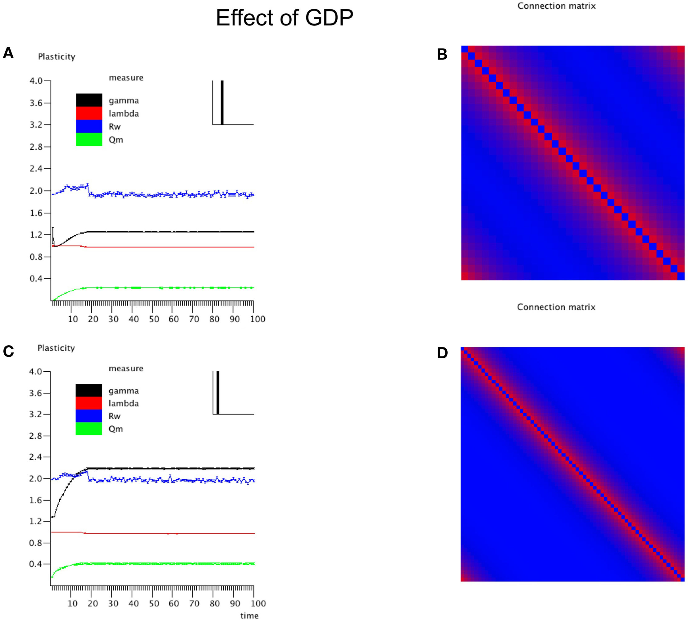
Figure 2. Effects of growth dependent plasticity (GDP) on network parameters. (A) For the network with N = 32, the evolution of gamma (black line), lambda (red line), degree correlation (blue line), and weighted modularity (green line) are shown for the first 100 epochs (each epoch consisted of 9096 time samples), averaged over 10 runs (error bars ± 2 SD). For gamma and lambda and modularity the y-axis indicates the scale. For the degree correlation R_w, 2 × (R_w + 1) is plotted. The inset in the right upper corner shows the final distribution of the connection strengths between the NMMs. (B) Final weighted connection matrix. The strength of the weights is indicated on a scale from 0 (blue) to 1 (red). (C,D) Show in a similar way the results for the larger network of N = 64.

The final node strength (sum of all connection strengths) distribution P(S) is shown in the inset in the right upper corner of Figure 2. This confirms that all nodes have about the same strength. Figures 2C,D show the results for the larger network of N = 64. Note that the formula for the GDP depends upon absolute, not relative distance; we used this approach to keep the average node strength within certain limits, irrespective of network size. Results for the large network are similar to those for the small network with a few exceptions. The normalized clustering coefficient rises to substantially higher values than in the small network, and reaches values around 2.2. The degree correlation fluctuates around 0, and does not take on positive values as was the case for the small network. The weighted modularity reaches a value of 0.403 (random network: 0.149).

In conclusion, starting from an initially unconnected network, GDP gives rise to a network with connection strengths that drop exponentially with distance, have typical small-world features but a narrow strength distribution and no visual indication of modular structure, although values of weighted modularity are higher than those of random networks.

Experiment 2: The Influence of SDP

In this experiment the effect of SDP was studied in isolation. Since SDP can only change the strength of existing connections, and does not involve the growth of new connections, an unconnected network could not be used as the initial state. Instead we used a network with average degree k = N/2, and a fully random distribution of connections over the network. All connections weights were random numbers from the interval [0,1]. For the SDP step size parameter, a_SDP, a value of 0.005 was chosen. In Figure 3A the plots for N = 32 are shown. While lambda stays around 1, gamma evolves toward a stable value of 1.2. The degree correlation rises to a positive value around 0.1. Weighted modularity reaches a value of 0.229 (random network: 0.175). The strength distribution (inset right upper corner) is rather broad. The final weighted connection matrix, shown in Figure 3B, reveals a pattern of widely scattered small clusters of connection strengths close to 1, surrounded by a background where the connection strength is close to 0 (please note that there has been no reordering of the nodes in this or any other of the figures). Results for the large network are shown in Figures 3C,D. While the general pattern is the same as for the small network, there are a few differences. Gamma and the degree correlation evolve to higher values, and still are increasing after 50 epochs. Weighted modularity reaches a value of 0.354 (random network: 0.161).

FIGURE 3

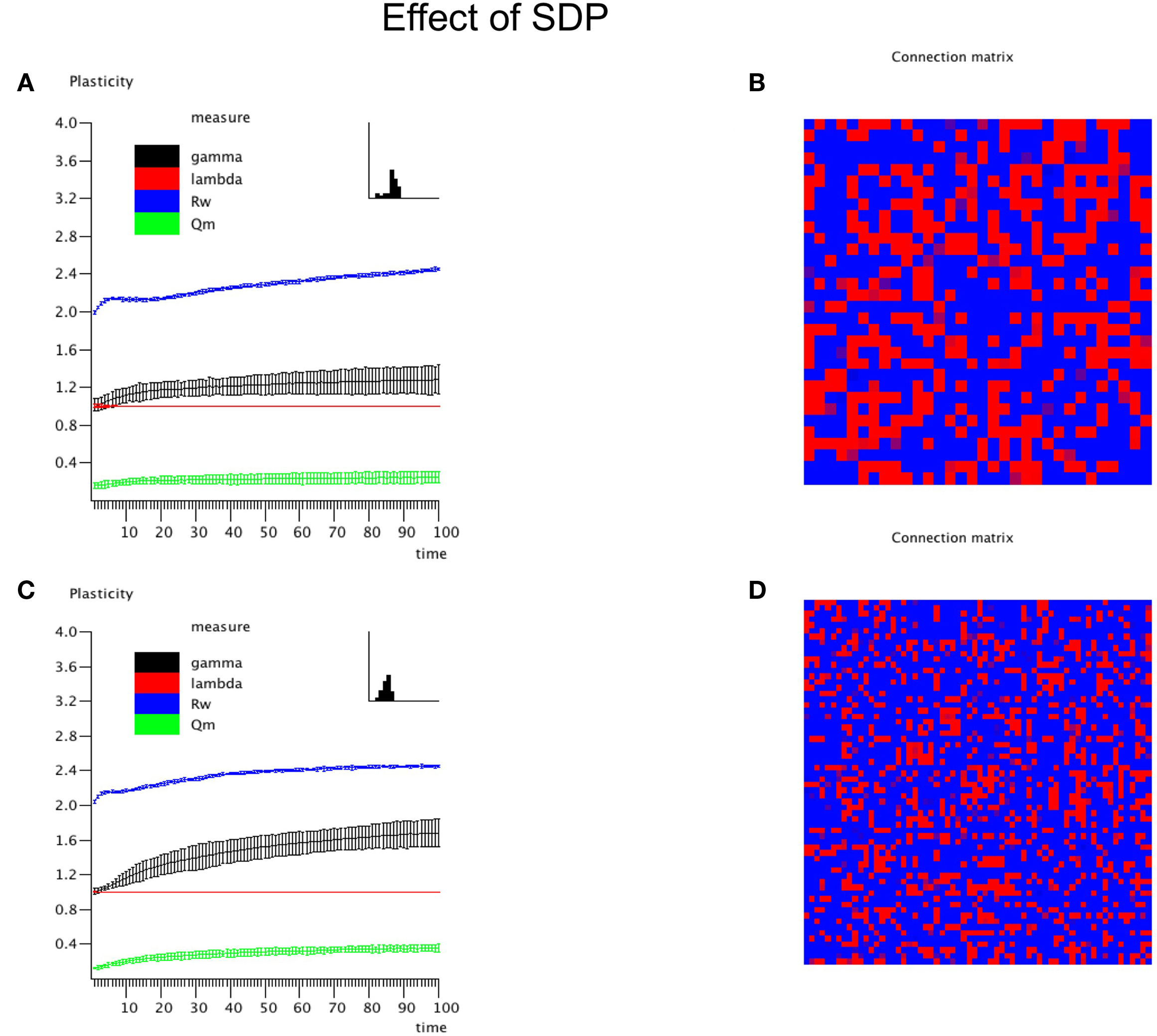
Figure 3. The influence of synchronization dependent plasticity (SDP) on network parameters. The initial network had an average degree of k = N/2, and connection weights taken at random from the interval [0,1]. For the SDP parameter a_SDP, a value of 0.005 was used. Results for the small network with N = 32 are shown in (A,B), results for the large network with N = 64 are shown in (C,D), in a similar way as in Figure 2.

Thus, SDP operating on a network with initial random connection topology and strength, results in a small-world network with scattered clustering, assortativity and broad strength distributions. The latter features were either absent or inconsistent with networks based upon GDP alone. SDP alone did however not result in networks with clear modules, although the value of weighted modularity was higher than for corresponding random networks.

Experiment 3: The Combined Effect of SDP and GDP

The central experiment involved the combined effect of GDP and SDP, starting from an initially unconnected network. In these experiments GDP step size was fixed at 0.001, while SDP step size varied from 0 to 0.012. First, in Figure 4 we show the evolution of small and large networks for an SDP step size of 0.008, and 100 epochs (100 × 9096 time steps), averaged over 10 realizations. Figure 4A shows that lambda stays around 1, except for a brief small increase around epoch 20. Gamma is initially high, drops very quickly, and then increases again around epoch 20, first quickly, then slower, to reach a value of 1.4. The degree correlation evolves toward positive values, and has a temporary maximum around epoch 20. Weighted modularity increases up to 0.278 (random network: 0.109). The final strength distribution is slightly broad. The final weighted connection matrix, shown in Figure 4B is of special interest. We can clearly see a complex pattern with a dense module in the upper left corner, a smaller overlapping module in the middle, and a large but fragmented module occupying the lower right corner. Results for N = 64 are shown in Figures 4C,D. The pattern is the same, but higher final values are obtained for gamma (2.37), weighted modularity (0.450; random network: 0.147) and the degree correlation (0.113). Also, the peak in the degree correlation around epoch 20 is more outspoken than in the small network. The weighted connection matrix (Figure 4D) shows a delicate pattern of multiple, partially overlapping modules. The appearance of the weighted connection matrix for small and large networks for different values of the SDP step size is illustrated in more detail in Figure 5. The transition of a mostly distance dependent connection pattern for SDP step size = 0.002 (upper and lower leftmost panels) toward a more complex modular pattern for SDP step size = 0.010 (upper and lower rightmost panels) is clearly visible.

FIGURE 4

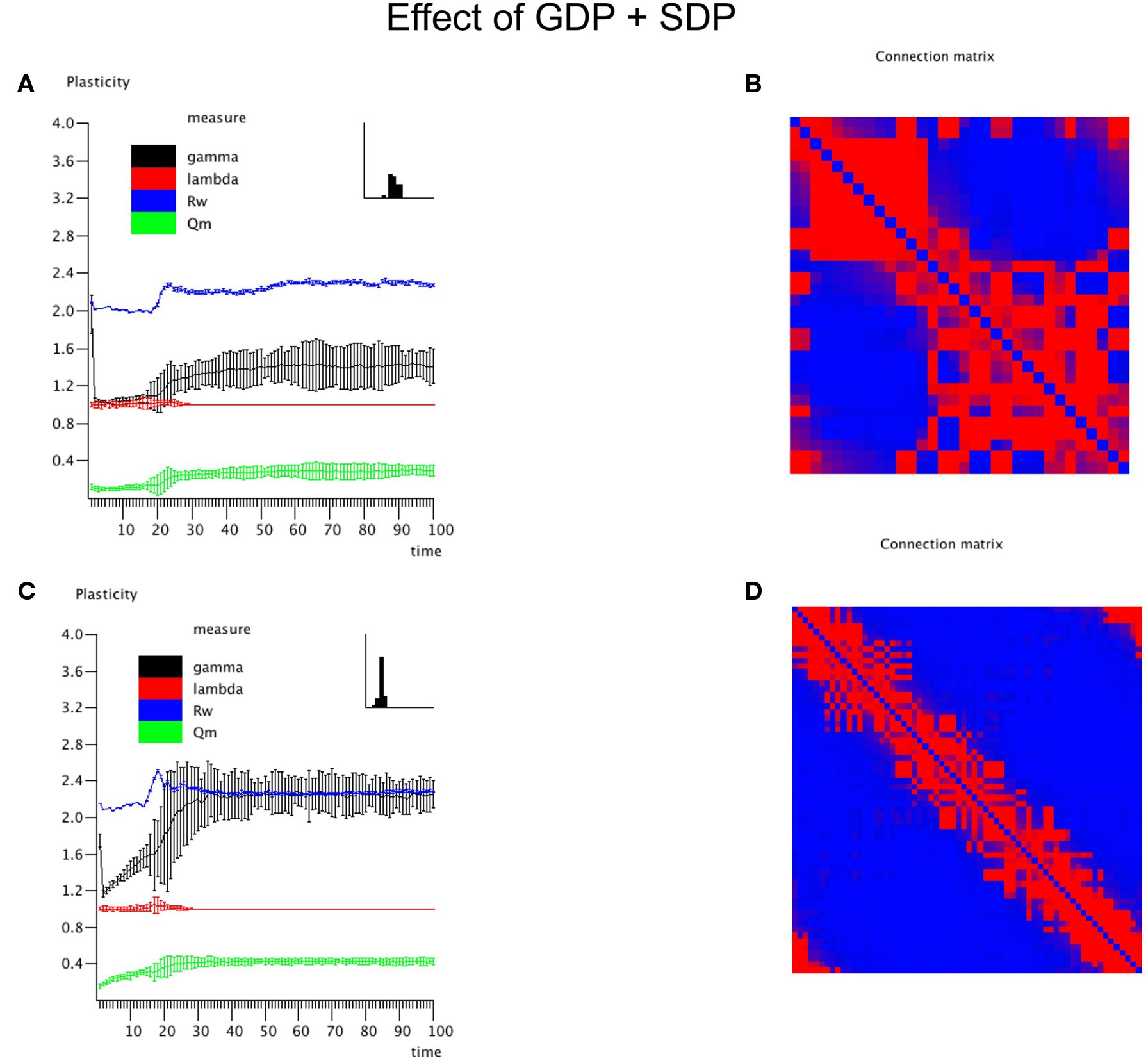
Figure 4. The combined effect of SDP and GDP on network parameters. The initial network had no connections. GDP step size was fixed at 0.001 and SDP step size at 0.008. Results for the small network with N = 32 are shown in (A,B), results for the large network with N = 64 are shown in (C,D), in a similar way as in Figure 2.

FIGURE 5

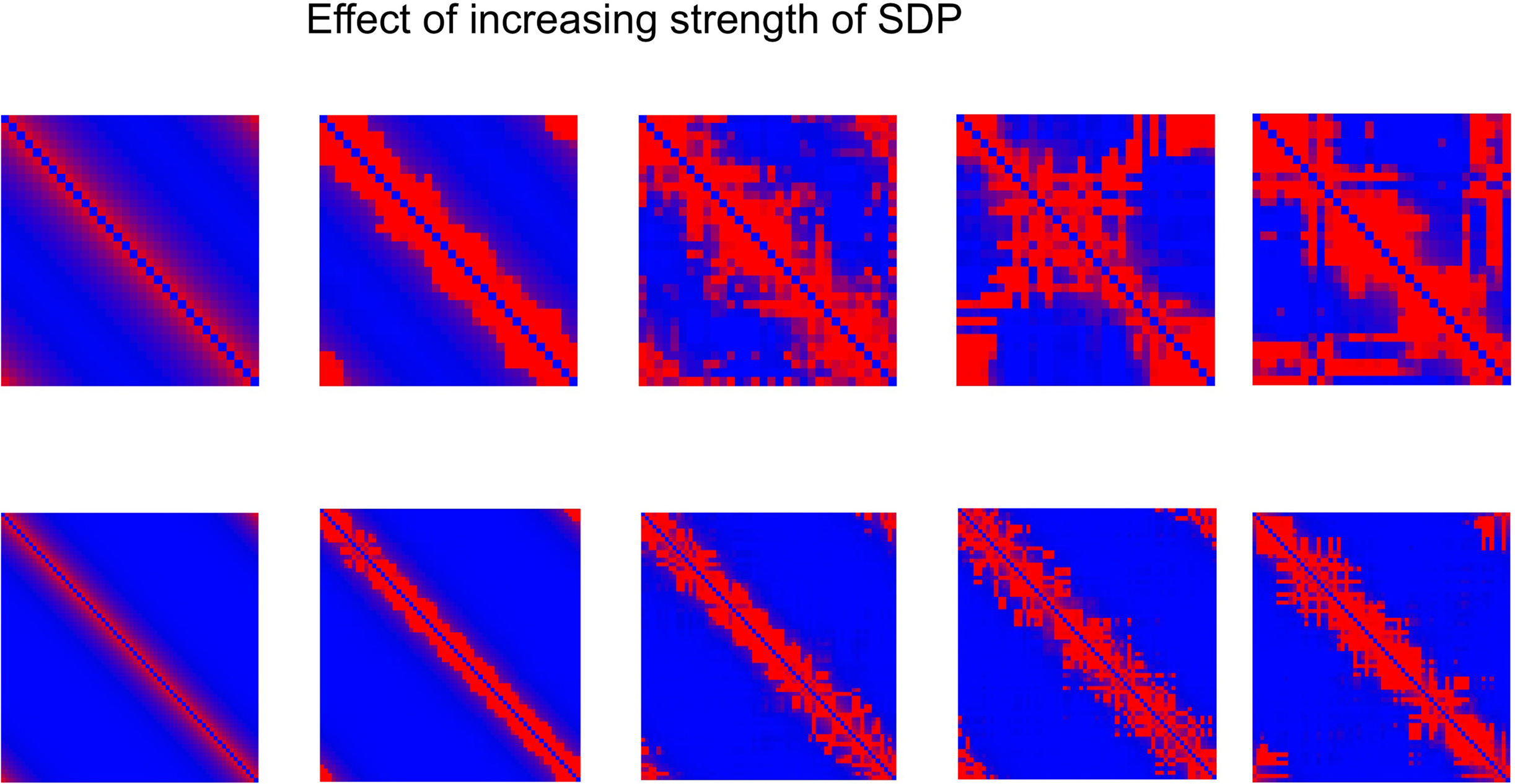
Figure 5. Weighted connection matrix for small (N = 32; top row) and large (N = 64; bottom row) networks for different values of the SDP step size (from 0. 002 to 0.010 in steps of 0.002). GDP step size was fixed at 0.001. Connection weight is indicated on a scale from 0 (blue) to 1 (red).

The weighted modularity index was also studied for the small network, 200 epochs, and SDP stepsize varying from 0 to 0.012 in steps of 0.001. The average result (error bars ± 2 SD) of 10 networks is shown in Figure 6. shows two maxima as a function of SDP step size, one for step sizes of 0.003–0.004, and higher one for step sizes of 0.009–0.010. Of interest, the first maximum corresponds to a division of the network into three modules, while the larger second maximum corresponds to a division of the network into two modules. The lower curve shows the results for random networks with the same average connection strengths. Except for SDP stepsize 0.004 and 0.005, and SDP stepsize > 0.010, the error bars (error bars ± 2 SD) do not overlap.

FIGURE 6

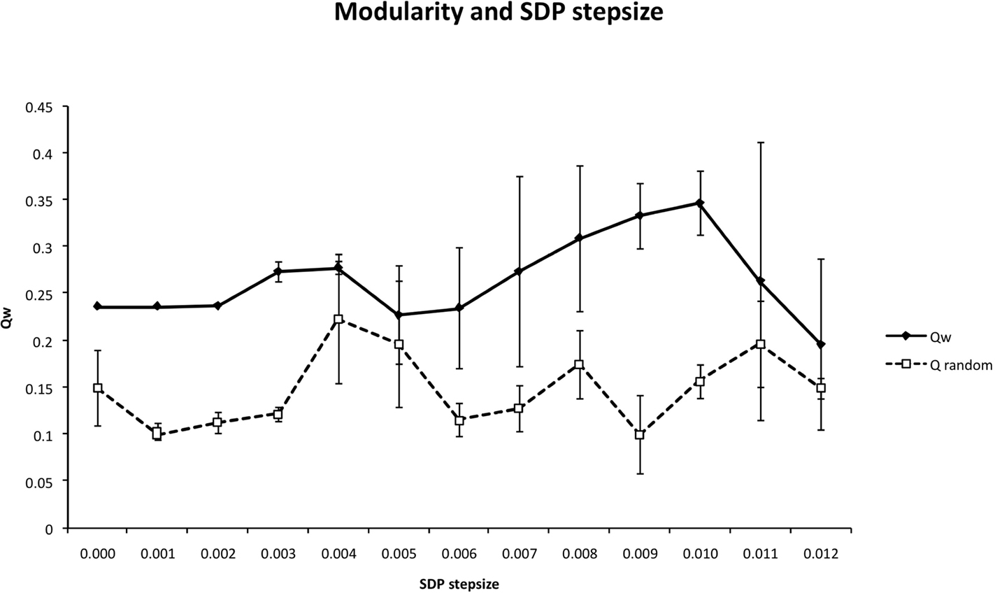
Figure 6. The weighted modularity index as a function of SDP step size for the small network (N = 32), 200 epochs, and SDP step size varying from 0 to 0. 012 in steps of 0.001 (error bars ± 2 SD).

Network development with an appropriate balance between GDP and SDP thus gives rise to small-world networks with high values of kappa, assortative degree coupling, and a complex modular structure. Size and number of modules depend upon the balance between GDP and SDP, as well as network size.

Experiment 4: Recovery from Lesions

An important question is how plastic brain networks recover from a sudden brain lesion. Lesions were modeled by setting all connections of neural masses 1–5 to very low values (0.1 × η, with η a random number from the interval [0,1]) at epoch number 51. Network parameters and evolution for epoch 1–50 were the same as in Experiment 3. Figure 7A shows the results for the small network. The first part up to epoch 50 shows a similar evolution as Figure 4A. The lesion at epoch 51 gives rise to a sharp increase in lambda, gamma, and the degree correlation; weighted modularity shows a modest decrease. During the next 50 epochs lambda, gamma, and modularity recover to their original values. The degree correlation shows a temporary increase after the lesion followed by a slow recovery of the values before the lesion. The final weighted connection matrix is shown in Figure 7B. It displays a complex pattern, with multiple partially overlapping modules of different size. The results for the large network, shown in Figures 7C,D, agree with those for the small network. A more detailed view of connectivity changes induced by the lesion is shown in Figure 8. The upper left corner shows a network of N = 32 after an evolution of 100 epochs, with the same settings as before. The upper middle pattern shows the immediate lesion effect: all connections of node 1–5 are weakened to very low values. The subsequent panels (upper right, lower left to right) show the network changes in steps of five epochs. There is a clear outgrowth of new connections, resulting in a partial restoration of the module in the upper left corner.

FIGURE 7

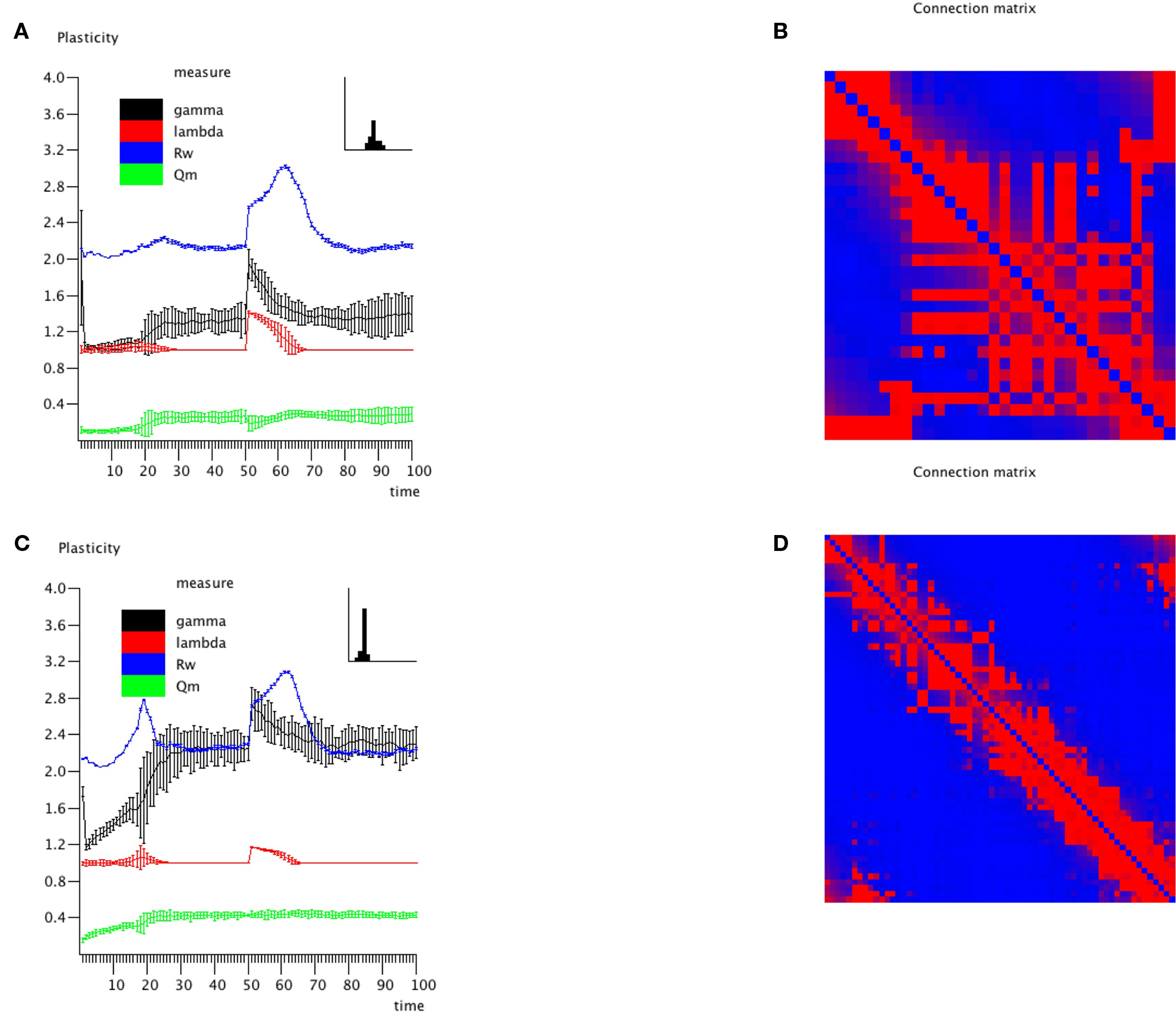
Figure 7. Effect of lesions on small (N = 32; A,B) and large (N = 64; C,D) networks. Lesions were modeled by setting all connections of neural masses 1–5 to very low values (0.1 × η, with η a random number from the interval [0,1]) at epoch number 51. Network parameters and evolution for epoch 1–50 were the same as in Experiment 3.

FIGURE 8

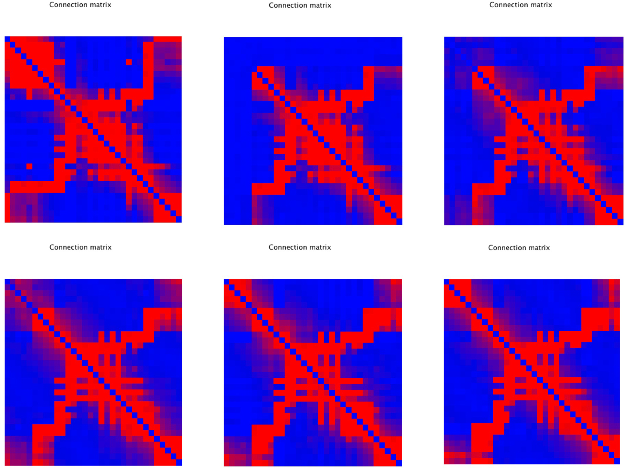
Figure 8. Detailed view of connectivity changes induced by the lesion. The upper left corner shows the adjacency matrix for a network of N = 32 after an evolution of 100 epochs, with the same settings as before. The subsequent panels (upper right, lower left to right) show the evolving adjacency matrix in steps of five epochs. Note the reappearance of modules as the network recovers from the induced damage.

Discussion

We have shown how a network of coupled neural masses can develop a complex topology through an interaction between the dynamic processes taking place on the network and the connection structure of the underlying network. We assumed two processes, GDP resulting in a distance dependent distribution of connection strengths, and SDP modifying connections on the basis of synchronization strength between modules. A proper balance between both processes resulted in networks with small-world features (high clustering and short path length), assortative mixing and modular structure. The strength of SDP in relation to GDP, as well as the network size, determined the number of modules in the final network. In addition, lesioning such networks resulted in a temporary disruption of network topology, which recovered over time with a restoration of modular architecture.

Growth Dependent Plasticity

The first process we included in our model was that of GDP. There is increasing evidence that neurons form highly dynamic elements, not only in terms of their electrical activity, but also in terms of their ever changing morphology. It has been suggested that neurons may regulate the outgrowth or retraction of dendrites and axons in such a way that they maintain a certain level of activity (Butz et al., 2009a). Such homeostatic aspects of structural plasticity could also determine the response of networks to lesions (Butz et al., 2009b). In our model we incorporated this in an indirect way, by evolving connections strengths such that the mean strength (sum of all connection weights of a node) of each node was kept within certain limits. The mean connection strength is a key determinant of the activity level of neural models, and limiting this strength therefore ensures that the activity level remained within certain limits.

A second important consideration is space. In many graph models space is not considered explicitly. However, the topology of developing and mature brain networks is hard to understand without taking distance into account. Kaiser and Hilgetag (2004) have shown that random, distance dependent outgrowth of connections in a two-dimensional geometric model can explain many of the topological features of real anatomical brain networks of cats and macaques. However, to explain the emergence of modules, ad hoc assumptions about the timing of connection growth had to be made (Kaiser and Hilgetag, 2007). More recently it has been shown how the exponential distribution of connections in brain networks can be explained by a random outgrowth of dendrites and axons (Kaiser et al., 2009). We incorporated this in the exponential shape of the GDP function (Eq. 3). The randomness in the process was reflected by the small, random update steps of GDP. As a result, the connections strengths in our model showed small, random, fluctuations around an average exponential decay as a function of distance (Figures 2B,D). GDP alone can explain how an initially unconnected network can evolve toward a network with small-world features, in agreement with the observations of Kaiser and Hilgetag (2004). However, GDP does not consistently produce assortative networks, and does not fully explain modularity. The presence of relatively high modularity in non-modular lattice-like networks is a well-documented conceptual shortcoming of the modularity metric. Although the final values of the weighted modularity were higher than those of a random network, no modular structure was visible in the connection matrix. Also, GDP only depends upon the connection topology and weights, and does not take the activity on the network into account.

Synchronization Dependent Plasticity

In contrast to GDP, SDP represents a true interaction between dynamics on the network and the underlying structural connection strengths. At the neuronal level, much has been learned about such mechanisms (Abbott and Nelson, 2000). Depending upon their correlated activity levels the synaptic strength between neurons can be adapted by pre- and post-synaptic mechanisms such as synaptic scaling and STDP. In addition, rewiring of existing connections and outgrowth of dendrites and axons play a role at the neuronal level (Butz et al., 2009a). Thus, both functional as well as structural mechanisms play a role with synaptic plasticity. A central idea is that of Hebbian learning: connection strengths between neurons that show correlated firing increase over time. While Hebbian learning may explain selective reinforcement of functionally important connections, this mechanism may be inherently unstable. Instability could be dealt with by synaptic scaling, and depletion of pre-synaptic resources (Levina et al., 2007). The mechanism of SDTP combines selective reinforcement with stability since excessive connectivity will disrupt the exact timing of pre- and post-synaptic neurons (Song et al., 2000). Models incorporating one or more of the synaptic mechanisms of plasticity typically evolve from an initial random topology toward a complex architecture with typical small-world features (Siri et al., 2007). In addition, SDTP and pre-synaptic depletion may explain how such evolving networks become critical (Shin and Kim, 2006; Levina et al., 2007; Sendina-Nadal et al., 2008). However, it is not clear how these findings should be translated to the macroscopic level of interacting cortical regions and observed correlations in EEG, MEG, and fMRI studies. Also, models at the neuronal level do not seem to explain the emergence of modular structure and assortative mixing.

The SDP in our model is an attempt to describe how the various mechanisms of functional and structural plasticity described above might be reflected at the level of interacting neural masses. We assume that neural masses will increase the strength of their excitatory interconnections when they oscillate more synchronously, and decrease this strength otherwise. This idea was implemented in the Hill type SDP function (Eq. 4). At this stage we cannot derive the SDP function from the multitude of synaptic mechanisms involved. However, it seems reasonable to assume that increased correlated firing at the neural level will be reflected by increased synchronization at the population level. We used the spike densities, not the average voltages, to determine the correlated activity of two neural masses, since the spikes may be closer to the actual neural interaction processes. SDP cannot give rise to new connections, so if we want to study its effect we have to assume some pre-existing topology and distribution of connection weights. This was explored in Experiment 2, where we applied SDP to sparsely connected networks with random topology and random connection strengths. SDP resulted in a decrease of some connections and an increase of other connections. Interestingly, SDP resulted in scattered small clusters (Figures 3B,D). SDP is a positive feedback process, and it seems likely that small groups of highly synchronous and connected nodes will tend to grow and recruit other nearby nodes in the process. This might explain why the resulting networks are small-world, but also assortative (Figures 3A,C). However, SDP does not result in true, large-scale modules, even though the weighted modularity is higher than that for a corresponding random network. In addition, this SDP-induced modularity is probably neurobiologically unrealistic, as the modules in Figure 3 seem to be formed between “spatially remote” regions. Furthermore SDP is an inherently unstable mechanism, which drives all connection weights to either their lowest allowed value (0) or their highest possible value (1). The instability of SDP without GDP is also clear from the fact that gamma and R_w do not reach stable values even after 100 runs (Figures 3A,C). Therefore, SDP alone does not provide a realistic account of mechanisms of plasticity, and it does not account for the modularity found in real networks.

SDP Plus GDP

The central idea of our model is that we need both GDP and SDP to simulate how activity and connectivity interact in developing plastic neural networks. This interaction is demonstrated in Experiment 3. Varying the strength of SDP for a constant strength of GDP gives rise to complex networks with small-world features and, most importantly, assortative mixing in combination with clear modularity (Figure 4). Modularity for the network with combined GDP and SDP was higher (0.278) than that for either GDP (0.236) or SDP (0.229) in isolation. Only the combination of GDP and SDP resulted in a clearly visible modular structure. The fact that modular networks emerged for a range of SDP strengths can be understood by considering how the two processes interact. For absent or very weak SDP the process is obviously dominated by GDP alone, resulting in non-modular networks (Figure 5). When SDP is too strong, any new weak connections generated by the GDP mechanism will be removed by the SDP function due to a weak correlation between firing patterns. Only for intermediate values of SDP (between 0.002 and 0.010) we have a situation where some of the new connections generated by GDP are strong enough to cause synchronization of neural masses, and subsequent strengthening by the SDP function. Interestingly, modularity as a function of SDP step size has two maxima, one at 0.003–0.004 and a second one at 0.009–0.010. It seems the dynamics of GDP and SDP interact at multiple “stable states”, each corresponding to a different number of large-scale modules.

Only a few other studies have attempted to explain the emergence of modular structure in complex networks. Fuchs et al. (2009) investigated synchronization dynamics in modular networks, but did not consider how the modular topology could arise in the first place. Aoki and Aoyagi (2009) studied the interaction between network topology and synchronization dynamics in a network of coupled phase oscillators. A two-cluster state could emerge in this model, suggestion that connectivity/dynamics interactions may be relevant for the emergence of modularity. However, the details of this simple model are hard to translate into possible neurobiological mechanisms of module formation. In a series of studies it has been shown that synchronization dependent rewiring of networks of coupled logistic functions can give rise to modular structure (van den Berg and van Leeuwen, 2004; Zhou et al., 2007; Rubinov et al., 2009b). While this is an elegant minimal scenario, it requires chaotic dynamics of the units, which may not be a realistic scenario for the dynamics of neural masses. We have previously shown that the NMMs used in our study have dynamics that is at most weakly non-linear, and not chaotic (Stam et al., 1999). In addition, the rewiring scheme that was used in the previously mentioned studies is biologically unrealistic since it does not take into account the influence of distance on neural connectivity, and does not handle outgrowth of new connections and loss of old connections. The model of Kaiser and Hilgetag (2007) does take into account the importance of distance, but, in order to explain modules, required the extra assumption of specific time intervals during which connections in different parts of the system grew. In our model, modularity evolved naturally without such timing assumptions.

Lesions

A combination of GDP and SDP gives rise to complex modular networks. Even in the stable state, with a relatively constant modular architecture, these networks are still dynamic, with the slow appearance and disappearance of connections and the constant adjustment of connection weights. It would be interesting to know how this ongoing plasticity would affect the response of the brain network to lesions, to better understand observations on network characteristics in neurological patients (Butz et al., 2009b). We have shown that an acute “lesion”, modeled by a sudden loss of connections of a few adjacent nodes, results in an immediate change in network topology with increased path length and clustering, increased degree correlation and decreased modularity. Over time, the network recovers most of its original structure, including the modularity, but the recovery rate and pattern is different for different network properties. While gamma, lambda, and modularity show an exponential approximation to the original values, the degree correlation shows a transient positive peak some time after the lesions. This peak is reminiscent of the peak that is also observed in the initial development, at the stage where the modular structure is rapidly evolving. Recovery from a lesion thus reflects to some extent a replay of events during network evolution. Other studies that have investigated the effect of lesions on complex networks have mainly concentrated on acute effects, and have not yet taken into account the role of plasticity in network recovery (Honey and Sporns, 2008; Alstott et al., 2009; Rubinov et al., 2009a). The study by Butz et al. (2009a,b) did take into account plasticity after lesions, and also reported a slow recovery of the initial network. However, this study involved networks of neurons, and does not describe changes in network topology on larger scales.

Modeling of lesion effects in plastic networks with activity–connectivity interactions could help to understand empirical observations with EEG, MEG, and fMRI in patients. There is now increasing evidence that brain lesions, in particular brain tumors but also traumatic brain injury, may have widespread effects on networks, and may disrupt the normal network topology (Bartolomei et al., 2006a,b; Bosma et al., 2009; Nakamura et al., 2009). The nature of these changes may depend upon time of observation and the frequency band studied, as well as therapeutic interventions (Douw et al., 2008). Network randomization has mainly been found in higher frequency bands (Bartolomei et al., 2006b; Bosma et al., 2009). In lower frequency bands, brain tumors may give rise to abnormal increase in clustering (Bosma et al., 2009). Of interest, the latter observation corresponds to the increase in the normalized clustering coefficient observed after lesions in our model.

Obviously, the current model is only a crude initial attempt to understand how activity–connectivity interactions can give rise to complex networks with modular and assortative structure, and how such models respond dynamically to damage. However, a major advantage is that the model makes predictions at the level of macroscopic measures such as EEG, MEG, and fMRI BOLD signals. This creates the opportunity to study fundamental mechanisms in the model, and make predictions with respect to output signals that can be directly tested in healthy subjects and patients. In a previous study we have shown that a consistent but complex relation exists between the topological properties of the adjacency matrix and the topological properties of functional networks derived from the output signals of the model (Ponten et al., 2010). Ideally, an iteration of modeling and empirical studies will increase our understanding of fundamental brain mechanisms underlying network development and plasticity. Major challenges for future studies are linking the evolution functions, in particular the SDP, more directly to known synaptic mechanisms, devising ways to test information processing in the model, and implementation of more sophisticated disease models of growing lesions, white matter disturbances and neurodegenerative disorders such as Alzheimer’s disease (Stam et al., 2009).

Conflict of Interest Statement

The authors declare that the research was conducted in the absence of any commercial or financial relationships that could be construed as a potential conflict of interest.

Acknowledgments

The authors would like to thank Mrs Els van Deventer for help with retrieving some of the cited papers. We would also like to thank the investigators of our “complex networks” group for many inspiring discussions.

References

Abbott, L. F., and Nelson, S. B. (2000). Synaptic plasticity: taming the beast. Nat. Neurosci. 3(Suppl.), 1178–1183.

Pubmed Abstract | Pubmed Full Text | CrossRef Full Text

Alstott, J., Breakspear, M., Hagmann, P., Cammoun, L., and Sporns, O. (2009). Modeling the impact of lesions in the human brain. PLoS Comput. Biol. 5, e1000408. doi: 10.1371/journal.pcbi.1000408.

Pubmed Abstract | Pubmed Full Text | CrossRef Full Text

Aoki, T., and Aoyagi, T. (2009). Co-evolution of phases and connection strengths in a network of phase oscillators. Phys. Rev. Lett. 102, 034101.

Pubmed Abstract | Pubmed Full Text | CrossRef Full Text

Bartolomei, F., Bosma, I., Klein, M., Baayen, J. C., Reijneveld, J. C., Postma, T. J., Heimans, J. J., van Dijk, B. W., de Munck, J. C., de Jongh, A., Cover, K. S., and Stam, C. J. (2006a). How do brain tumors alter functional connectivity? A magnetoencephalography study. Ann. Neurol. 59, 128–138.

CrossRef Full Text

Bartolomei, F., Bosma, I., Klein, M., Baayen, J. C., Reijneveld, J. C., Postma, T. J., Heimans, J. J., van Dijk, B. W., de Munck, J. C., de Jongh, A., Cover, K. S., and Stam, C. J. (2006b). Disturbed functional connectivity in brain tumour patients: evaluation by graph analysis of synchronization matrices. Clin. Neurophysiol. 117, 2039–2049.

CrossRef Full Text

Bettencourt, L. M. A., Stephens, G. J., Ham, M. I., and Gross, G. W. (2007). Functional structure of cortical neuronal networks grown in vitro. Phys. Rev. E Stat. Nonlin. Soft Matter Phys. 75, 021915.

Pubmed Abstract | Pubmed Full Text | CrossRef Full Text

Boccaletti, S., Latora, V., Moreno, Y., Chavez, M., and Hwang, D.-U. (2006). Complex networks: structure and dynamics. Phys. Rep. 424, 175–308.

CrossRef Full Text

Bonifazi, P., Goldin, M., Picardo, M. A., Jorguera, L., Cattani, A., Bianconi, G., Represa, A., Ben-Ari, Y., and Cossart, R. (2009). GABAergic hub neurons orchestrate synchrony in developing hippocampal networks. Science 326, 1419–1426.

Pubmed Abstract | Pubmed Full Text | CrossRef Full Text

Bosma, I., Reijneveld, J. C., Klein, M., Douw, L., van Dijk, B. W., Heimans, J. J., and Stam, C. J. (2009). Disturbed functional brain networks and neurocognitive function in low-grade glioma patients: a graph theoretical analysis of resting-state MEG. Nonlin. Biomed. Phys. 3, 9. doi: 10.1186/1753-4631-3-9.

CrossRef Full Text

Bullmore, E., and Sporns, O. (2009). Complex brain networks: graph theoretical analysis of structural and functional systems. Nat. Rev. Neurosci. 10, 186–198.

Pubmed Abstract | Pubmed Full Text | CrossRef Full Text

Butz, M., Wörgötter, F., and van Ooyen, A. (2009a). Activity-dependent structural plasticity. Brain Res. Rev. 60, 287–305.

CrossRef Full Text

Butz, M., van Ooyen, A., and Worgotter, F. (2009b). A model for cortical rewiring following deafferentation and focal stroke. Front. Comput. Neurosci. 3:10. doi: 10.3389/neuro.10.010.2009.

CrossRef Full Text

de Arcangelis, L., and Herrmann, H. J. (2010). Learning as a phenomenon occurring in a critical state. Proc. Natl. Acad. Sci. U.S.A. 107, 3977–3981.

Pubmed Abstract | Pubmed Full Text | CrossRef Full Text

Douw, L., Baayen, H., Bosma, I., Klein, M., Vandertop, P., Heimans, J., Stam, K., de Munck, J., and Reijneveld, J. (2008). Treatment-related changes in functional connectivity in brain tumor patients: a magnetoencephalography study. Exp. Neurol. 212, 285–290.

Pubmed Abstract | Pubmed Full Text | CrossRef Full Text

Fuchs, E., Ayali, A., Ben-Jacob, E., and Boccaletti, S. (2009). The formation of synchronization cliques during the development of modular neural networks. Phys. Biol. 6, 036018.

Pubmed Abstract | Pubmed Full Text | CrossRef Full Text

Grindrod, P., and Higham, D. J. (2009). Evolving graphs: dynamical models, inverse problems and propagation. Proc. R. Soc. Lond. A Math. Phys. Sci. doi: 10.1098/rspa.2009.0456 [3133].

Guimera, R., and Nunes Amaral, L. A. (2005). Functional cartography of complex metabolic networks. Nature 433, 895–900.

Pubmed Abstract | Pubmed Full Text | CrossRef Full Text

Hagmann, P., Cammoun, L., Gigandet, X., Meuli, R., Honey, C. J., and van Wedeen, J. (2008). Mapping the structural core of human cerebral cortex. PLoS Biol. 6, e159. doi: 10.1371/journal.pbio.0060159.

Pubmed Abstract | Pubmed Full Text | CrossRef Full Text

Honey, C. J., Kotter, R., Breakspear, M., and Sporns, O. (2007). Network structure of cerebral cortex shapes functional connectivity on multiple time scales. Proc. Natl. Acad. Sci. U.S.A. 104, 10240–10245.

Pubmed Abstract | Pubmed Full Text | CrossRef Full Text

Honey, C. J., and Sporns, O. (2008). Dynamical consequences of lesions in cortical networks. Hum. Brain Mapp. 29, 802–809.

Pubmed Abstract | Pubmed Full Text | CrossRef Full Text

Honey, C. J., Sporns, O., Cammoun, L., Gigandet, X., Thiran, J. P., Meuli, R., and Hagmann, P. (2009). Predicting human resting-state functional connectivity from structural connectivity. Proc. Natl. Acad. Sci. U.S.A. 106, 2035–2040.

Pubmed Abstract | Pubmed Full Text | CrossRef Full Text

Jun, J. K., and Jin, D. Z. (2007). Development of neural circuitry for precise temporal sequences through spontaneous activity, axon remodeling, and synaptic plasticity. PLoS ONE 8, e723. doi: 10.1371/journal.pone.0000723.

CrossRef Full Text

Kaiser, M., and Hilgetag, C. C. (2004). Spatial growth of real-world networks. Phys. Rev. E Stat. Nonlin. Soft Matter Phys. 69, 036103.

Pubmed Abstract | Pubmed Full Text | CrossRef Full Text

Kaiser, M., and Hilgetag, C. C. (2007). Development of multi-cluster cortical networks by time windows for spatial growth. Neurocomputing 70, 1829–1832.

CrossRef Full Text

Kaiser, M., Hilgetag, C. C., and van Ooyen, A. (2009). A simple rule for axon outgrowth and synaptic competition generates realistic connection lengths and filling fractions. Cereb. Cortex 19, 3001–3010.

Pubmed Abstract | Pubmed Full Text | CrossRef Full Text

Kinouchi, O., and Copelli, M. (2007). Optimal dynamical range of excitable networks at criticality. Nat. Phys. 2, 348–352.

CrossRef Full Text

Leung, C. C., and Chau, H. F. (2007). Weighted assortative and disassortative networks model. Physica A 378, 591–602.

CrossRef Full Text

Levina, A., Herrmann, J. M., and Geisel, T. (2007). Dynamical synapses causing self-organized criticality in neural networks. Nat. Phys. 3, 857–860.

CrossRef Full Text

Li, Y., Liu, Y., Li, J., Qin, W., Li, K., Yu C., and Jiang, T. (2009). Brain anatomical network and intelligence. PloS Comput. Biol. 5, e1000395. doi: 10.1371/journal.pcbi.1000395.

Pubmed Abstract | Pubmed Full Text | CrossRef Full Text

Lopes da Silva, F. H., Hoeks, A., Smits, A., and Zetterberg, L. H. (1974). Model of brain rhythmic activity. Kybernetik 15, 27–37.

Pubmed Abstract | Pubmed Full Text | CrossRef Full Text

Nakamura, T., Hillary, F. G., and Biswal, B. B. (2009). Resting Network plasticity following brain injury. PLoS ONE 4, e8220. doi: 10.1371/journal.pone.0008220.

Pubmed Abstract | Pubmed Full Text | CrossRef Full Text

Ponten, S. C., Daffertshofer, A., Hillebrand, A., and Stam, C. J. (2010). The relationship between structural and functional connectivity: graph theoretical analysis of an EEG neural mass model. Neuroimage 52, 985–994.

Pubmed Abstract | Pubmed Full Text | CrossRef Full Text

Reijneveld, J. C., Ponten, S. C., Berendse, H. W., and Stam, C. J. (2007). The application of graph theoretical analysis to complex networks in the brain. Clin Neurophysiol 118, 2317–2331.

Pubmed Abstract | Pubmed Full Text | CrossRef Full Text

Rubinov, M., McIntosh, A. R., Valenzuela, M. J., and Breakspear, M. (2009a). Simulation of neuronal death and network recovery in a computational model of distributed cortical activity. Am. J. Geriatr. Psychiatry 17, 210–217.

CrossRef Full Text

Rubinov, M., Sporns, O., van Leeuwen, C., and Breakspear, M. (2009b). Symbiotic relationship between brain structure and dynamics. BMC Neurosci. 10, 55.

CrossRef Full Text

Schuuring, D. (1988). Modelleren en simuleren van epileptische activiteit. Masters thesis, Rapport 080 DV-8807, communicatietechniek, Informatie en Systeemtheorie, technische Universiteit Twente.

Sendina-Nadal, I., Buldu, J. M., Leyva, I., and Boccaletti, S. (2008). Phase locking induces scale-free topologies in networks of coupled oscillators. PLoS ONE 3, e2644. doi: 10.1371/journal.pone.0002644.

Pubmed Abstract | Pubmed Full Text | CrossRef Full Text

Shin, Ch-W., and Kim, S. (2006). Self-organized criticality and scale-free properties in emergent functional neural networks. Phys. Rev. E Stat. Nonlin. Soft Matter Phys. 74, 045101.

Pubmed Abstract | Pubmed Full Text | CrossRef Full Text

Siri, B., Quoy, M., Delord, B., Cessac, B., and Berry, H. (2007). Effects of Hebbian learning on the dynamics and structure of random networks with inhibitory and excitatory neurons. J. Physiol. Paris 101, 136–148.

Pubmed Abstract | Pubmed Full Text | CrossRef Full Text

Smit, D. J. A., Boersma, M., van Beijsterveldt, C. E. M., Posthuma, D., Boomsma, D. I., Stam, C. J., and de Geus, E. J. C. (2010). Endophenotypes in a dynamically connected brain. Behav. Genet. 40, 167–177.

Pubmed Abstract | Pubmed Full Text | CrossRef Full Text

Smit, D. J. A., Stam, C. J., Posthuma, D., Boomsma, D. I., and de Geus, E. (2008). Heritability of ‘small-world’ networks in the brain: a graph theoretical analysis of resting-state EEG functional connectivity. Hum. Brain Mapp. 29, 1368–1378.

Pubmed Abstract | Pubmed Full Text | CrossRef Full Text

Song, S., Miller, K. D., and Abbott, L. F. (2000). Competitive Hebbian learning through spike-timing-dependent synaptic plasticity. Nat. Neurosci. 3, 919–926.

Pubmed Abstract | Pubmed Full Text | CrossRef Full Text

Sporns, O., Chialvo, D. R., Kaiser, M., and Hilgetag, C. C. (2004). Organization, development and function of complex brain networks. Trends Cogn. Sci. 8, 418–425.

Pubmed Abstract | Pubmed Full Text | CrossRef Full Text

Srinivas, K. V., Jain, R., Saurav, S., and Sikdar, S. K. (2007). Small-word network topology of hippocampal neuronal network is lost, in an in vitro glutamate injury model of epilepsy. Eur. J. Neurosci. 25, 3276–3286.

Pubmed Abstract | Pubmed Full Text | CrossRef Full Text

Stam, C. J., de Haan, W., Daffertshofer, A., Jones, B. F., Manshanden, I., van Cappellen van Walsum, A. M., Montez, T., Verbunt, J. P. A., de Munck, J. C., van Dijk, B. W., Berendse, H. W., and Scheltens, P. (2009). Graph theoretical analysis of magnetoencephalographic functional connectivity in Alzheimer’s disease. Brain 132, 213–224.

Pubmed Abstract | Pubmed Full Text | CrossRef Full Text

Stam, C. J., Pijn, J. P. M., Suffczynski, P., and Lopes da Silva, F. H. (1999). Dynamics of the human alpha rhythm: evidence for non-linearity? Clin. Neurophysiol. 110, 1801–1813.

Pubmed Abstract | Pubmed Full Text | CrossRef Full Text

Stam, C. J., and Reijneveld, J. C. (2007). Graph theoretical analysis of complex networks in the brain. Nonlin. Biomed. Phys. 1, 3. doi: 10.1186/1753-4631-1-3.

CrossRef Full Text

Ursino, M., Zavaaglia, M., Astolfi, L., and Babiloni, F. (2007). Use of a neural mass model for the analysis of effective connectivity among cortical regions based on high resolution EEG recordings. Biol. Cybern. 96, 351–365.

Pubmed Abstract | Pubmed Full Text | CrossRef Full Text

van den Berg, D., and van Leeuwen, C. (2004). Adaptive rewiring in chaotic networks renders small-world connectivity with consistent clusters. Europhys. Lett. 65, 459–464.

CrossRef Full Text

Van den Heuvel, M. P., Stam, C. J., Kahn, R. S., and Hulshoff Pol, H. E. (2009). Efficiency of functional brain networks and intellectural performance. J. Neurosci. 29, 7620–7625.

CrossRef Full Text

Yu, S., Huang, D., Singer, W., and Nikolic, D. (2008). A small world of neuronal synchrony. Cereb. Cortex 18, 2891–2901.

Pubmed Abstract | Pubmed Full Text | CrossRef Full Text

Zetterberg, L. H., Kristiansson, L., and Mossberg, K. (1978). Performance of a model for a local Neuron population. Biol. Cybern. 31, 15–26.

Pubmed Abstract | Pubmed Full Text | CrossRef Full Text

Zhou, C., Zemanova, L., Zamora-Lopez, G., Hilgetag, C., and Kurths, J. (2007). Structure–function relationship I complex brain networks expressed by hierarchical synchronization. New J. Phys. 9, 178.

CrossRef Full Text