Closed-form treatment of the interactions between neuronal activity and timing-dependent plasticity in networks of linear neurons

Introduction

At the network level recent theoretical advances have made it possible to analytically calculate the activity patterns for certain types of simplified neuron models as long as one keeps the synaptic connectivity fixed (Memmesheimer and Timme, 2006a,b). Concerning plasticity, the situation is reversed. When fixing the activity pattern or rather, when considering long-term activity averages, it is for many plasticity rules possible to calculate the overall development of synaptic weights. Older results exist which provide specific solutions for estimating synaptic strengths in certain types of networks and learning rules, all of which however need to constrain structure or dynamics of the system in different ways (Hopfield, 1982; Miller and MacKay, 1994; Roberts, 2000; van Rossum et al., 2000; Kempter et al., 2001; Burkitt et al., 2007; Kolodziejski et al., 2008) and many of them do not resemble spike-timing-dependent plasticity (STDP, Magee and Johnston, 1997; Markram et al., 1997). Concerning STDP, in large networks one finds that over longer times the distribution of synaptic efficiencies usually develops into either an unimodal (van Rossum et al., 2000; Gütig et al., 2003) or a bimodal (Song et al., 2000; Izhikevich et al., 2004) shape. These results mainly rely on simulations (Song et al., 2000; van Rossum et al., 2000) or mean-field approximations (van Rossum et al., 2000; Gütig et al., 2003). Additionally, in order to keep the weights beyond a given value, soft (van Rossum et al., 2000; Morrison et al., 2007) or hard (Song et al., 2000; Izhikevich et al., 2004; Burkitt et al., 2007; Lubenov and Siapas, 2008; Gilson et al., 2009; Clopath et al., 2010) boundaries have to be introduced.

All these observations pose a problem, because STDP can generically lead to the situation that individual pre- and post-synaptic spike pairs influence the synaptic strength of their connection and thereby in a recurrent way immediately also the activity in the network. The question arises, thus, whether such fast synaptic changes would carry any functional significance or whether they will be averaged out by the ongoing network activity? At the moment this issue is left open because resolving it would require measuring or calculating the step-by-step changes of synaptic connectivity together with their activity for a large number of neurons and ideally for every spike pair.

Experimentally this is at the moment still impossible and so far there are also no theoretical tools available (apart from simulations) to address the issue of ongoing mutual interactions between activity and plasticity in networks. For this, analytical methods would be particularly helpful with which it would be possible to predict the dynamics of synaptic connections under STDP.

As discussed above, this is typically investigated with mean-field methods (van Rossum et al., 2000; Gütig et al., 2003) that have average values in their focus. However, here we would like to examine the fine temporal dynamics of each weight as, fundamentally, the concept of STDP needs to rely on temporally local (pulse–pulse) interactions. Thus, in the current study we will start addressing the issue of temporal locality by providing a general analytical framework for calculating plasticity in a time-continuous way in networks with an arbitrary number of synapses using Hebbian plasticity rules. These are, for example, plain Hebbian or differential Hebbian learning, where the latter is known to have properties similar to STDP (Roberts, 1999; Wörgötter and Porr, 2004).

Naturally, the complexity of the solution is high and, while it could be used to investigate the interplay of activity and plasticity in any network topology, we will here first look at three, still rather simple, cases of recurrent networks, which have been chosen because they could be considered as fundamental network building blocks. This allows us to arrive at several interesting observations which may be the starting point for the investigation of more complex topologies of which we will give a brief example at the end.

For example, we find that in the investigated simple recurrent networks many fixed points exist where synapses stabilize in spite of the recurrently arriving inputs and that boundaries (soft or hard) are not required. More intriguing, this can lead to the situation that such a network can better stabilize when there is an asymmetric STDP curve in which the long-term potentiation (LTP) part dominates.

We will address these topics by organizing the paper in the following way. In Section “Materials and Methods” we define the system we are going to solve analytically, depict the three different network structures the analytical solution is applied to and also describe the specifics of the recurrent connections. In Section “Results” we provide the analytical solution of our general Hebbian system and also verify several useful approximations. Next we use our solution to calculate all configurations in the investigated network structures that lead to non-divergent weights. Here, we describe the results under different conditions, i.e., with/out noise and with an asymmetric STDP rule. Finally, in Section “Discussion”, we put the results to a broader context. Detailed calculations can be found in Section “Appendix”.

Materials and Methods

STDP-Like Plasticity Rule

The general one-neuron system used as the basis of this study consists of N synapses with strength ω_i that receive input from neurons i with continuous values x_i. Each input produces an excitatory post-synaptic potential (EPSP) which is modeled by filter functions h_i (see Figure 1A for an example). The output of the neuron is, thus:

where describes a convolution.

FIGURE 1

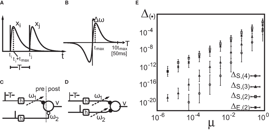
Figure 1. Setup (A–D) and verification (E) of the approximation of Eq. 4. (A) Two pulses x_i and x_j at times t_i and t_j respectively are convolved with filter h. (B) Depending on the time difference T, differential Hebbian plasticity leads to a STDP-like weight change curve Δω (Porr and Wörgötter, 2003; Kolodziejski et al., 2008). The maximum is at t_max = (log(β) − log(α))/(β − α). (C) A simple network with only a single plastic synapse with which the relation of differential Hebbian plasticity to spike-timing-dependent plasticity is shown. (D) The used feed-forward network with two plastic synapses. (E) Here we show the degree of consistency between our general solution and the proposed approximations. To this end we plot the difference (see Approximations for the Analytical Solution) between the approximation and the exact solution of Eq. 3 for one input pulse pair against the plasticity rate μ on a log-log scale. Here, a filter function h with α = 0.1, β = 0.2, σ = 0.25, and max_th(t) = 1 is used (Eq. 8). The temporal difference T = t_i − t_j, between the two input pulses was varied over the length of the used filter functions (here between 1 and 100 steps) and error bars representing the standard deviation are given.

Synapses change according to a generally formalized Hebbian plasticity rule

where μ (set to 0.01 throughout the article) is the plasticity rate and F[ξ] and G[ξ] are linear functionals. However, although the analytical solution that we will present later on holds for the generally formalized plasticity rule (Eq. 2), we will only consider F = 1 (where 1 is the identity) and G = d/dt. This is called differential Hebbian learning (Kosco, 1986; Klopf, 1988) and allows for the learning of temporal sequences of input events (Porr and Wörgötter, 2003). It resembles STDP (Roberts, 1999; Wörgötter and Porr, 2004). Another important setting for F and G is conventional Hebbian learning with F = G = 1.

To avoid that weight changes will follow spurious random correlations one generally assumes that learning is a slow process, where inputs change much faster than weights, with dω_i/ω_i << d(x_i * h_i)/x_i * h_i, μ → 0. In spite of this separation of time scales, such a simplification makes it still possible to investigate the dynamics of each weight separately. The separation simplifies Eq. 2 and we neglect all temporal derivatives of ω_i on the right hand side which leads to where we used as G[ξ] is linear.

If we take ω_i as the i-th component of a vector ω, we write its most general form

with A_ij(t) = F[x_i * h_i](t)G[x_j * h_j](t) or in matrix form where denotes the transposition of matrix ξ. In the results section we will show that following closed-form solution is possible

however, as such is quite complex. Nevertheless, we will also show that for our quasi-static assumption μ → 0 the approximation where I is the identity matrix, is arguable.

Relation to spike-timing-dependent plasticity

In order to show that F = 1 and G = d/dt resembles STDP we use a simplified version of the system, namely a system with N = 2 (see Figure 1C), however, where only one of the synapses is plastic (ω₁); the other stays fixed (ω₂ = 1). In order to get the correct STDP protocol, we now present two pulses to this system, one at t = 0 to the input connected with the plastic synapse, hence a pre-synaptic spike, and another at t = T to the other input. As we are using a linear model and as the corresponding weight ω₂ is set to a fixed value of 1, a pulse at the input is also a pulse at the output, hence creating the pendant of a post-synaptic spike. The equivalence of relating differential Hebbian plasticity with STDP arises essentially from this and its implications are discussed in detail in Saudargiene et al. (2004) and Tamosiunaite et al. (2007). Recently also Clopath et al. (2010) related voltage-based Hebbian learning to STDP.

For such a network structure, it is possible to analytically calculate the shape of the STDP curve. We start with Eq. 3 where we focus on the first entry of ω(t): ω₁(t). The second synapse stays fixed: ω₂(t) = ω₂.

First, we calculate the influence of a single pulse on the weight ω₁. To this end we set x₂(t) = 0 for all t and x₁(t) = δ(t) which is a spike at t = 0. It simplifies the convolution to a temporal shift in the filter function This leaves us with a first order differential equation with following solution:

Filters usually have the property that they decay to 0 after a while which turns the exponential function into 1 and results in no weight change. Thus, a single pulse or a rate produced by a single input does not have any influence on the weight when not combined with another pulse. For these pulse–pulse correlations we have to set the other input to have a pulse at t = T: x₂(t) = δ(t − T). If we use a simplification (with all the details in Kolodziejski et al., 2008) the result of the differential Eq. 5 for very long times writes

where we used here and throughout the manuscript

Hence, different values of the pulse timing T lead to different Δω values, which, when plotted in Figure 1B against T, resemble a fully symmetrical STDP curve (for more details see Porr and Wörgötter, 2003; Saudargiene et al., 2004; Tamosiunaite et al., 2007; Kolodziejski et al., 2008). The shape and symmetry of the STDP curve depends purely on the filters’ shape, thus on the post-synaptic potentials’ (PSPs) shapes (see Figure 1A). Thus, with different filters h for x₁ and for x₂ one could get either LTP or long-term depression (LTD)-dominated curves (see Figure 2c in Porr and Wörgötter, 2003).

We used h(t) with parameters α = 0.009, β = 0.0099, and σ = 0.029. The maximum of h(t) is at t_max = (log(β) − log(α))/(β − α). The width of the STDP curve measured at biological synapses is usually about T = ±50 ms (Bi and Poo, 1998; Caporale and Dan, 2008). Thus, as our filter ceases to 10⁻⁴ at around t ≈ 1000, we define 1000 time steps as 50 ms (which corresponds to α = 0.18 ms⁻¹and β = 0.198 ms⁻¹) to which we will refer throughout the text.

Not only the shape of the STDP curve is determined by the filter function (Eq. 8) but also the shape of the pulses. As our model is linear, each pulse could be thought of as a weighted delta function (pseudo spike) convoluted with the filter function.

Network Structures and Inputs

Although our method would allow investigating general network structures, we will concentrate on only three very simple, but fundamental ones.

The first structure consists of a single neuron with two plastic synapses (see Figure 1D). Although quite simple, the analytical solution of this feed-forward structure demonstrates the power of the method developed in this paper. The next structure is a small network with two neurons and only one plastic synapse (see Figure 2A). This network structure is equivalent to just one neuron with a plastic recurrent connection of total delay d. This is due to our assumption of linearity. The last structure we consider is a network with three neurons and two plastic synapses (see Figure 2C). Here the equivalence is to a single neuron with two plastic recurrent connections. Note, these two structures could be considered as part of a larger recurrent network, where – after some intermittent stages – activity arrives back at its origin (with unchanging synapses in between). Hence, recurrent structure like those could be seen as simple network building blocks and in the end we shortly discuss larger network structures (i.e., a ring of neurons) that have similar stability properties as those building blocks.

FIGURE 2

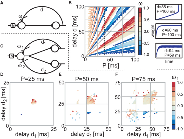
Figure 2. Stable fixed points of the single (A) and double (C) recurrence networks without noise. (B) The color code indicates the actual weight values of each fixed-point dependent on the parameter P and d (delay) of the network. Parameter configurations which lead to divergent weights are not shown (i.e., are white). The three panels on the right side of (B) exemplify the three possible temporal weight developments (from top to bottom: divergent, convergent, and oscillating). (D–F) Dependent on two delays d₁ and d₂ the stable fixed points for the three neuron structure (C) are shown. Each panel uses a different P value (D: 25 ms; E: 50 ms; F: 75 ms). Note that we only need to plot one of the two weights as the other weight is just a reflection in the diagonal; the diagonal as such represents the single recurrence weights (half of the value).

For the input we will use input spike distributions with first moment P (expectation value) that comes in three different conditions. The firing will be without any noise and thus, periodic, with Gaussian noise using a mean value of P and a standard deviation of σ = 5 ms and, additionally, we will also apply a purely Poisson distributed firing with rate P (hence no periodic input).

As our model is linear, it can not as such produce spikes on its own. However, we could at any point introduce a threshold so that each time a pulse exceeds this threshold a spike would travel along the axon to the next neuron via its synapses. In our first order approximation we do not need this threshold, however, we could apply it afterward.

Input Pulse Timing and Amplitude

The external input to the system is a sequence of δ-function spikes, which are being transformed into PSPs by convolving the normalized filter function h with the input sequence. As the model is linear, outputs are graded pulses, which result from the weighted linear summation of all inputs at the soma of the neuron (Eq. 1). As we do not use spike thresholds, these outputs directly provide the recurrent part of the input to the system.

We need to calculate the complete input time function, notable the timing and amplitude of all pulses that enter a neuron. We investigate recurrent systems with an external input of periodicity P with delays d_i, i = 1,…,R (in this study we only consider R = 1 and 2 but the analysis holds for R ∈ ℕ). To get a better intuition for recurrences in networks like those described above (Figures 2A,C) we can compare each recurrence to a modulo operation. We find all pulse timings pt by iterating the map pt_c+1 = mod (pt_c + d_i, P) until The total number of relevant pulse times N_s = P/gcd(P,d₁,…,d_R) depends on the greatest common divisor (gcd) of P and all R delays d_i. For instance, all relevant pulse times for P = 75 and d = 60 are pt_c = {0, 60, 45, 30, 15}. This gives us the timings of the pulses. In order to calculate the amplitude Γ of each pulse of a system with R recurrent connections, we need to go further and solve this linear system of equations: Γ = (I − Λ)⁻¹λ where Λ is a matrix that handles the delayed recurrences and λ the external input; I is the identity matrix. The details of the derivation are provided in Section “Pulse Timings and Amplitude” in the Appendix. Having calculated the pulse amplitudes we are now able to calculate the weight change.

Results

Analytical Solution of Weight Dynamics

Here we are going to develop a closed-form for the matrix which governs the temporal development (Eq. 4) of the weights ω(t) according to Eq. 3. This solution is not trivial as the matrix A(t) is also a function of time. This problem is often found in quantum mechanics and the main problem is that matrices usually do not commute. A solution exists, however, it includes an infinite series, called the Magnus series (see Magnus, 1954 for more details), with

where ω(t₀) are the synaptic strengths at time t₀, hence before plasticity, and Ω(t) is the solution of following equation

Here the braces are nested commutators [η,ξ] = ηξ − ξη and β_n are the coefficients of the Taylor expansion of Ω/(1 − exp(−Ω)) around Ω = 0. Equation 10 is solved through integration by iteration to the Magnus series:

with Thus, Eq. 9 combined with Eq. 11, gives us analytically the time development of all weights connected to a neuron under Hebbian plasticity in the limit of small plasticity rates μ. With this we are able to calculate without simulations in principle directly the synaptic strengths of N synapses given N different pulse trains. This property will be useful to analytically calculate the fixed-point values of the weights of our small network structures.

Approximations for the analytical solution

Before we apply the solution to our network structures, we transform it into a computable form and provide error estimates. As the commutators in the infinite series in Eq. 11 are generally non-zero we truncate the series and neglect iterations above degree (k). We write the truncated solution as For two synapses this is solved directly later on, most often, however this needs to be calculated by expanding the exponential function. We denote this approximation, where we neglect terms of both the exponential as well as the Magnus series greater than of order (k), with an S instead of an E, i.e., S,(k), thus Notice that in the limit k → ∞ the approximation transforms into the general solution (Eq. 9). This solution is computable for arbitrary input patterns.

Now, as we know the complete analytical solution of Eq. 3, we investigate approximations and their errors in order to judge their usefulness for further considerations. To estimate the approximation errors we can use δ functions as inputs to the system. Furthermore, we assume that all h_i = h are equal. The pulses are again modeled as δ functions δ(t − t_i) for times t_i which simplifies the convolution to a temporal shift in the filter function This leads for elements of A(t) to A_ij(t) = F[h](t − t_i)G[h](t − t_j) where t_i and t_j are the pulse timings of neuron x_i and x_j respectively. We will use the filter shown in Figure 1A, given by Eq. 8.

The different approximation errors are exemplified in Figure 1E. For this we are using a single pulse pair at two synapses (see Figure 1C) for which we calculate the final synaptic strength (Eq. 9). This has been performed for differential Hebbian learning, but we remark that the error is identical for Hebbian learning. For this setup, weight changes are computed in three ways: without any approximations, yielding (Eqs. 9 and 11); using the truncated solution only, yielding and using the truncated solution while also expanding the exponential function, yielding Thus, we use and compare it to approximations calculating the error as: This is plotted in Figure 1E for different approximations against the plasticity rate μ on a log-log scale where we set the maximal value of the input filter h to 1. As approximations E,(k) and S,(k) become very similar for k > 2, only four curves are shown. We observe that the behavior of the difference-error Δ_.,(k) follows the order of the approximation used. The error for the linear expansion approximation S,(k = 2) is slightly higher than that from its corresponding truncation approximation E,(k = 2). However, using a plasticity rate of μ = 0.001 already results in a difference-error value of 10⁻⁸ compared to 10⁻² when using the same value for μ and the maximum of h. Therefore, one can in most applications use even the simplest possible linear approximation S,(k = 2) to calculate the change in synaptic strength.

As this calculation has been based on two pulses at two synapses only, we need to ask how the error develops when using N synapses and complex pulse trains. For this we first consider pulse trains, which are grouped “vertically” into groups with each input firing at most once. Filters of pulses within a group will overlap but we assume that grouping is possible such that adjacent groups are spaced with a temporal distance sufficient to prevent overlap between filter responses of temporally adjacent groups. Thus we calculate ω in the same way as above leading to: When using such a temporal tiling, depends only on the pulse timing matrix T with elements T_ij = t_j − t_i. Then, we get the synaptic strength after M groups by calculating the product over all groups m to

This solution is easy to compute. Because a product of matrices results in a summation of matrix elements, the error does not increase exponentially but only linearly in M. Because of this it follows that even after 10000 pulses the error is still of an order of only 10⁻⁴ given the example above (see Figure 1E).

Finally we estimate how the error behaves when filters overlap. This mainly happens during bursts of pulses with temporarily high spiking frequencies, which are, in general, rare events. However, using the solution which assumes independent temporal intervals instead of the time-continuous calculation (Eq. 4), only includes an additional error of order k = 2 due to the linearity of the filter functions h. The error after matrix multiplication results in the square of the lowest term of the Magnus series (Eq. 11).

Thus, the easily computable group decomposition will yield accurate enough results even for long, non-bursting pulse trains.

Fixed-Point Analysis

Now we are able to calculate the temporal development of the weight dynamics in our networks. Most interesting are those developments that eventually lead to a stable, thus non-diverging, weight dynamics. Here, we develop the equations with which configurations of parameters (i.e., periodicity and delays of the recurrences) can be identified that lead to stable weights.

As mentioned, some of those (P, d_i) configurations converge to stable weight configurations, others do not. In order to reveal whether a configuration is stable, hence whether the plastic weights do not diverge, the nullclines () need to have stable crossing points in the open region ]−1, +1[^R with R being the number of recurrent connections (±1 would lead to diverging activity since a constant input is added periodically for a theoretically infinite number of times). A crossing point outside this interval is never stable because of the recurrent connections involved [ω(n + 1) = ξω(n) with ξ > 1 always diverges].

For the calculations we place all input pulses on a discrete grid, but calculate correlations by continuous analytical integration. Hence, the weight change in the discretized version of Eq. 4 is ω(n) = (n,m)·ω(m) where (n,m) denotes (t) with lower and upper boundaries m and n respectively. Weights are (periodically or asymptotically) stable if they take the same value after a certain number of periods P: ω(n) = ω(n + ξ·P) for ξ ≥ 1 and n large enough. Here in this study we concentrate on the analytical solution for ξ = 1.

Therefore, in order to calculate those fixed-point weights, the following system of equations needs to be solved:

with n large enough so that the weights have already converged. is defined to include all relevant pulse correlations; it is, thus, similar to . The roots of this system represent the fixed-points which are stable if all eigenvalues of are negative.

In the next step we will use the E,(k = 2) simplification for which is I + μ ∫_UA(τ)dτ with U being an interval that includes all relevant correlations. A detailed definition is given in Section “Fixed-Point Analysis” in the Appendix. With this we will arrive at an analytical solution of the weight dynamics of the recurrent structures. If we include this simplification into Eq. 12 we get

Now we have to write down matrix A to get its integral. With R recurrences and a single input, A is of dimension R + 1. The first R rows and columns describe the in- and outputs to the plastic synapses and the last row and the last column the in- and output to the constant input synapse. We define its input as K, which is a sum of δ functions always at the beginning of each period. The inputs to the plastic synapses are given by the pulse amplitudes Γ (Eq. A.2), however, delayed by different delay times d_i. Putting everything together, we have to solve following integral:

We skip the detailed calculations (including the definition for ) here, given in Section “Fixed Point Analysis” in the Appendix, and directly write the result where only correlations in the interval U have been considered and the pulse amplitudes Γ (Eq. A.2) were applied:

Obviously, the number of fixed points is not restricted to one and there exist many configuration with more than one fixed-point. However, we will show below that if a configuration is stable, than it does not matter how many fixed points in the interval ]−1, 1[ exist.

Here we would like to stress again that we are not interested in average quantities (no mean-field approach) but in the fine temporal dynamics of each single weight and additionally that a non-diverging weight is also a necessary condition for a non-diverging overall activity as we do not use any kind of boundaries.

Now, we have all tools ready to analyze the network structures (Figures 1C and 2A,C) starting without additional noise, thereafter with noise and finally by also considering asymmetrical STDP rules.

Analysis of the Network Structures without Noise

First, we will investigate the structures, which we introduced in the beginning of this study, in the absence of noise. The feed-forward structure always displays oscillation of weights and activity whereas the recurrent structures show more complex behavior. Depending on the network parameters, the weights either diverge, converge to a fixed-point or oscillate.

Feed-forward single neuron model

Here we look in more detail at symmetrical differential Hebbian plasticity with two plastic synapses (see Figure 1D) where the simplification E,(k = 2) is analytically fully solvable. We have also based the error analysis provided in Figure 1E on these calculations. For the approximation E,(k = 2) the matrix results in

where and Here we use two input neurons (N = 2), which receive inputs at t = 0 and T, respectively. Overall, this results in following solution for the weight after a pulse pair with the calculations provided in Section “Feed-Forward Structure” in the Appendix (special solution for ρ = 1)

Having found the analytical solution we now determine dynamics of the temporal development by calculating the eigenvalues λ_i of which are:

This shows clearly that the weights oscillate around 0 and that the oscillations of the weights are damped if the real parts of the eigenvalues λ_i are smaller than 0. This constraint holds for almost all T values as is only true for a multiple of the number 2 π. However, holds since we assume μ to be small. Furthermore, is trivial and does not lead to any weight change at all. Hence, the weights will continuously shrink to 0.

Recurrent Networks

Next, we investigate the stability of the two neuron model with a single recurrence (see Figure 2A) for which we need the previously provided solution for Eq. 13. In small panels to the right of Figure 2B we show three different temporal developments of the plastic weight. The top panel depicts a divergent weight (P = 100 ms and d = 85 ms), the middle panel a convergent weight development (P = 100 ms and d = 60 ms) and the bottom panel an oscillating weight (P = 59 ms and d = 94 ms). In the main panel of Figure 2B the weight values of all configurations for 0 < P < 100 ms and 0 < d < 100 ms (which is 0–2.0 times the characteristic STDP length of 50 ms) are plotted. In case of convergence the final weight is depicted, however, if the weight diverges, no point is plotted at all (white regions). For oscillating weights we plot the mean value.

Figure 2B reveals that if (P, d) is stable, then (nP, nd) with n ≥ 1 is also stable (lines through origin). However, weights will not be the same for (P, d) and (nP, nd). The stability statement only holds for configurations in which the weight has not reached a value whose absolute value is ≥1. This immediately leads to divergence and is the reason why the lines through the origin not always start at the origin.

Additionally, Figure 2B shows that excitatory and inhibitory regions always alternate and that the two regions for d < P (below diagonal) are almost of the same size as the many regions for d > P (above diagonal). Furthermore, if the first delayed pulse is closer to its input pulse (i.e., d < P/2), than the final weight is inhibitory. By contrast, if the first delayed pulse is closer to the consecutive input pulse (i.e., P/2 < d < P), than the final weight is excitatory. In the excitatory case, the pulse at the plastic synapse is followed by another pulse. This resembles a causal relationship which should lead to a weight growth. The opposite is true for the inhibitory case.

We also conducted a perturbation analysis in which we perturbed the weight for each configuration with increasing amplitude until the weight could not converge back to its fixed point. It turns out that the crucial measure for stability is whether the absolute value of the sum of the fixed-point value and the perturbation amplitude exceeds 1. This is true for almost all configurations with stable weights which is why we do not need to plot the results of the perturbation analysis.

Another property of the system is that the final weights are identical for (P, d + nP) configurations for all n ≥ 1 (see Figure 2B, in particular the black dashed line at P = 40 ms). Thus, if the weight for e.g., P = 40 ms and d = 25 ms converges to ω, so does the weight for P = 40 ms and d = 65 ms. We use this property to simplify the convergence plots of the network structure with three neurons or two quasi recurrences (Figures 2D–F) and only depict fixed points for delay values up to the periodicity P. We show the fixed points for three different values of P: 0.5, 1.0, and 1.5 times the characteristic STDP time window (we leave out the 2.0 times as we do not get anything novel at higher periodicity values according to Figure 2B).

Starting with P = 25 ms (Figure 2D) it is apparent that only a few inhibitory connections evolved (only about 10%). However, when moving to higher P values (Figures 2E,F), more and more inhibitory connections show up. If we had plotted (not shown) the ratio of excitatory connections, we would find that at about P = 100 ms the ratio of excitatory connections reaches 0.5 and for all smaller values the ratio is always >0.5, thus more excitatory connections develop. We note that all properties mentioned in this paragraph remain essentially the same, when adding noise to the input.

Figures 2E,F reveal that the main regions (upper-right, middle) move to higher (d₁, d₂) configurations and enlarge at the same time. In addition, new regions originate at smaller (d₁, d₂) configurations.

The total number of fixed points N₀ scaled by the number of the possible configurations, of which there are P², also grows with increasing periodicity (see Figure 3, black dots). In the next section we will compare the number of fixed points to two different noisy input protocols.

FIGURE 3

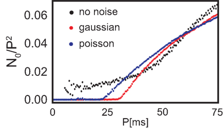
Figure 3. Number of configurations N₀ that lead to stable weights multiplied with the probability that such a configuration leads to stability (see Figure 4) with respect to the periodicity P. Additionally, N₀ is normalized by the maximum possible configurations (P²) and we plot the results without noise (black), with Poisson distributed firing with rate P (blue) and Gaussian distributed periodicity with mean P and a variance of 5 ms (red).

Analysis of the Network Structures with Noise

Above we used deterministic timing at the input to our system. As this is not realistic, we will now use two different types of noise. The first one is Gaussian jitter around the given periodicity value P with a standard deviation of 5 ms. The second one is Poisson firing with rate P. Due to the stochastic nature of the signals, analytical results cannot be obtained anymore and we have to rely on simulations.

Feed-forward Structure

The general behavior of the feed-forward structure does not change in the presence of either noise. Although the oscillations are not “perfect” anymore, weights are still oscillating and eventually they decay to 0.

Recurrent Structures

For the recurrent structures the situation is different as noise is able to change an initially unstable configuration to now exhibit a convergent weight development and vice versa. In Figure 4 we show the stability of the weights for different configurations. Here, red stands for highly stable weights (i.e., all trials lead to convergence) and blue for rarely stable ones (i.e., only a few trials lead to convergence). Stability in between where half of the trials lead to convergence is very rare, so we included those configurations to the rarely stable ones. In order to compare the noise results with those for no noise, we include the no noise stable regions in gray in Figure 4. Additionally, the color of each configuration that is stable both with and without noise is lighter (i.e., light red and light blue). We do not plot the actual final weight values as those are not largely different from the no noise ones.

FIGURE 4

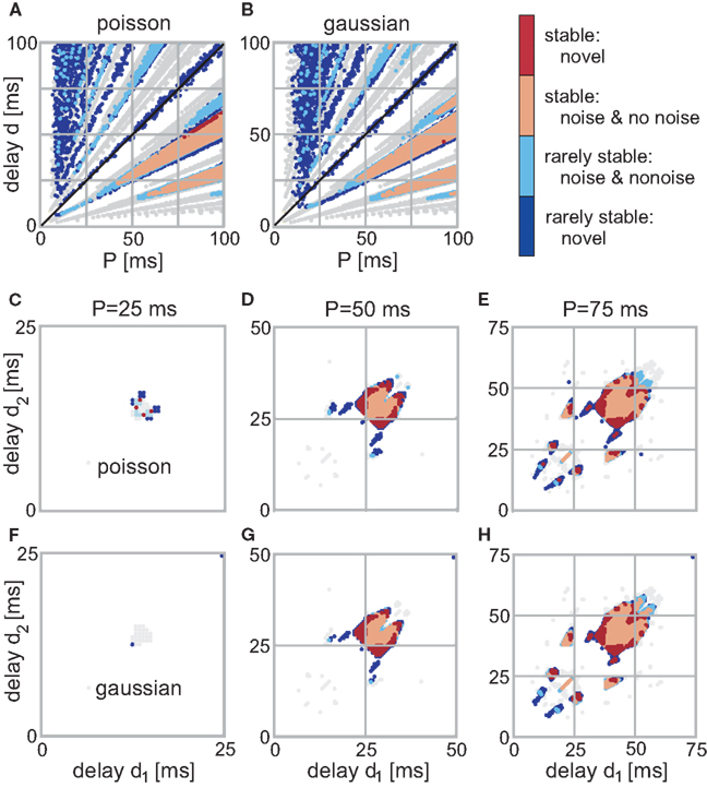
Figure 4. Stable fixed-points of the single (A,B) and double (C–H) recurrence network with noise. The color code indicates the stability of each point. (Light)red is for points which are stable at each trial (out of 10 simulations) and (light)blue for rarely stable points. In gray are the no noise fixed points; light colors indicate that a point is stable with and without noise. (A,B) Those panels show the weight stability where the firing was distributed following Poisson statistics (A) using P as rate. (B) Shows the results with Gaussian noise with a mean P and a variance 5 ms. (C–H) Three neuron structure; the left column depicts the converged weights for P = 25 ms, the middle for P = 50 ms, and the right for P = 75 ms. (C–E) Poisson distributed firing with rate P, (F–H) Gaussian distributed periodicity with mean P and a variance of 5 ms.

For the two neuron structure, a few of the branches in Figures 4A,B completely disappeared, others moved slightly. The two main branches for d < T (below diagonal) remain highly stable, however, only in the “core”. The more diffuse, non-compact regions, i.e., regions with detached stable configurations become either completely unstable or at least rarely stable. Noise affects the input periodicity, thus configurations that are stable for a large range of different P values survive when noise has been added. By contrast, configurations within non-compact regions are always deflected toward unstable configurations, thus, compromising or even losing their stability. However, in a few trials they still happen to survive which leads to the regions with many rarely stable configurations.

It is clearly visible that the number of stable configurations for the structure with a single recurrence substantially decreases. This is, however, not the case for the double recurrence structure. There, the number of stable configurations increases (see red border in Figures 4G,H) because of the compact structure. However, this effect starts above P = 30 ms which is revealed by Figure 3. In this figure we plot the number of stable (non-divergent) configurations N₀ normalized by the maximum possible configurations (P²) against the periodicity P. Only between about 30 and 60 ms noise increases the number of stable configurations by about 20%. Above 60 ms the smaller non-compact areas that lose stability dominate over the border areas that gained stability. Above a certain periodicity the smaller areas become large enough so that noise becomes advantageous again and border regions become stable. Therefore, the effect that noise slightly increases stability reoccurs periodically. Figure 3 also shows clearly that Poisson statistics leads to slightly more stable configurations than adding Gaussian noise. Most important, however, is the fact that noise does not deteriorate the system, i.e., the number of stable configurations stays almost unchanged.

Similar to the feed-forward structure, weights sometimes change from positive to negative values (or vice versa), hence they switch from being excitatory to being inhibitory which is not known from biology. However, this could be easily solved if we exchange our linear synapse with two non-linear synapses (one that is linear in the positive regime and 0 elsewhere and the other vice versa), so that such a push–pull mechanism covers the full linear range. This is the conventional way of addressing this issue (Pollen and Ronner, 1982; Ferster, 1988; Palmer et al., 1991; Heeger, 1993; Wörgötter et al., 1998). Note, however, in general we found that without noise switching is rather rare in our recurrent structures anyways. Even with additional noise weights tend to switch only if the final weight is close to 0.

Analysis of the Network Structures with Asymmetric STDP Rules

In biological systems, the STDP curve is not symmetrical (Bi and Poo, 1998; Caporale and Dan, 2008). In order to achieve an asymmetric differential Hebbian plasticity curve, we leave the positive part which describes the strengthening of the weight (LTP) as it is and shrink or stretch the negative part which describes the weakening (LTD). This is done by multiplying negative weight changes with a factor ρ.

Feed-forward Structure

For the feed-forward structure we calculated the temporal development analytically (see Section “Feed-Forward Structure” in the Appendix) and find that the general behavior is not changed by the asymmetry. This becomes visible from the eigenvalues of the system:

Both oscillation and damping still exist, however, damping constant and frequency of the oscillation is scaled by the asymmetry ρ.

Recurrent Structures

Now we come to the recurrent structures. Here, similar to the introduction of noise, the situation is different. With an additional asymmetry the number of stable configurations changes. In the following, we depict the number of stable configuration achieved with a certain asymmetry ρ = 2^a (logarithmic representation) by N_a. Thus, the number of stable configuration for the symmetric STDP curve is still N₀. Then, to better compare the different results, we normalize N_a to the symmetric number N₀ plotting N_a/N₀ in Figure 5. It is worthwhile to note that the total (not the relative) number of stable configurations without noise is reduced for any value of a for the single recurrence structure and stays almost unchanged for the double recurrence structure (see Figure 3).

FIGURE 5

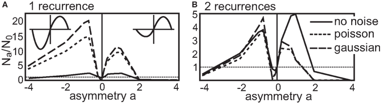
Figure 5. Number of stable configurations N_a with respect to the asymmetry a of the STDP curve normalized by the number of stable configurations without asymmetry N₀. The part that leads to a reduction in synaptic efficiency (LTD-side) is scaled by 2^a. (A) This panel shows the number of stable configurations of the single recurrence and (B) for the double recurrence structure both up to a periodicity of P = 50 ms. The results that were obtained without noise are depicted by the solid line, the results with Gaussian noise by the dash-dotted line and the results with Poisson statistics by the dotted line. The N₀ values for no noise, Gaussian and Poisson are 737, 73, 105 for the single recurrence network and for the double recurrence network they are 6464, 5693, 7435.

First, we look in more detail at the single recurrence structure (Figure 5A). We plot the normalized number N_a/N₀ of stable configurations up to a periodicity of P = 50 ms. The respective N₀ values can be found in the caption of Figure 5. The no noise results have a peak for positive and for negative asymmetries, thus an asymmetric STDP curve yields more stable configurations than a symmetric one. Here, a dominant LTP part is advantageous over a dominant LTD part. This situation changes when we introduce noise. An STDP curve with a dominant LTD part results now in more stable configurations than a LTP-dominant STDP curve. However, almost all asymmetric STDP curves lead to many more stable configurations as compared to a symmetric STDP curve. Here we note again that making the input spiking obeying the Poisson statistics is advantageous over adding Gaussian noise (if comparing absolute numbers).

Next, we consider the double recurrence structure (Figure 5B) where the number of stable configurations were also counted up to P = 50 ms. Here, the no noise result looks more similar to the results with noise; two peaks, one for an LTP-dominant and one for an LTD-dominant STDP curve, are visible. However, adding noise to the system again changes the relative heights of the peaks: the STDP curve with more LTD becomes advantageous over the STDP curve with more LTP. Similar to the single recurrence structure, there are more stable configurations when using Poisson noise, however, with Gaussian noise the boost in stability for asymmetrical as compared to the symmetrical STDP curve is larger. If we compare the number of stable configurations between LTP-dominant and LTD-dominant STDP curves we find that without noise about 55.0% LTP-dominant configurations of the total number of configurations exists. With Gaussian noise this ratio decreases to 41.7% and with Poisson statistics to 44.0%.

The dynamics of the structures examined here (and the reasoning should extend to all possible structures) would allow only for diverging weights if we set a → ±∞. As this would correspond to an STDP curve with pure LTP or LTD respectively, the dynamics pushes the weight only in one direction (either positive or negative) which leads to no fixed point (see Eqs. 14 and 15). This is also indicated in Figure 5 where the number of configurations leading to convergence is severely reduced even for a = ±4.

Discussion

Real neurons often display rich, non-stationary, firing patterns by which all synaptic weights will be affected. The so far existing solutions which describe Hebbian learning, on the other hand, constrain the temporal dynamics of the system or limit plasticity to a subset of synapses. With the solution presented here we can calculate weight changes for the first time without these restrictions. This is a valuable step forward in our understanding of synaptic dynamics of general Hebbian plasticity as well as of STDP (which is a special case of the general Hebbian plasticity rule) in different networks. Specifically, we have presented the time-continuous solution for the synaptic change of general Hebbian plasticity (Eqs 9 and 11), its approximation for general spiking or continuous inputs as well as a specific solution for non-bursting pulse trains. Of practical importance is the fact that the error of the computable approximations remains small even for long pulse trains.

We think that there is in general no intuitive access, which would allow us to understand the temporal development of activity and plasticity in networks with recurrent connections. Even small structures driven by periodic activity, such as the ones investigated here, display unexpected and counterintuitive behavior. The systems investigated are linear and summation takes place at the level of PSPs, which are here modeled by ways of the filter function h. This way closed-form solutions can be found. Spiking could be introduced by ways of a threshold. Introducing such a threshold essentially leads to the reduction of activity (eliminating all small linearly summed signals) but the general recurrence is not altered.

The first network investigated was a simple feed-forward structure (see Figure 1C) which displays oscillating weights which decay to 0. This observation is interesting and not expected as this network and its inputs represent a fully symmetrical situation. Hence, oscillation should occur, one would think, but without damping. Asymmetrical STDP curves do not alter this observation, because the asymmetry of the STDP curve only affects the frequency of the weight oscillation.

The focus of the current study, however, was to investigate recurrent network structures without averaging the activity. The two small recurrent networks studied here can be seen as fundamental network building blocks. This is due to the fact that the direct recurrent connections used here could also be replaced by a network, the output of which providing the recurrent signals. This seems to be similar to Roberts (2004), Burkitt et al. (2007), and Gilson et al. (2009), however, in those studies only average activities are considered. Roberts (2004) does not treat plasticity, Burkitt et al. (2007) and Gilson et al. (2009) do not have self-connections, and Roberts (2004) and Burkitt et al. (2007) do not have delays included. Without delays, self-connections would be cumbersome to implement in a general way (i.e., for different delays a different number of neurons need to be interposed). However, Burkitt et al. (2007) and also Gilson et al. (2009) could easily extend their models to include self-connections.

As a side remark, almost all of the above mentioned studies only consider pair-wise STDP correlations although a method for three-pair couplings exists (Pfister and Gerstner, 2006). By contrast, differential Hebbian plasticity treats multi-correlations naturally.

In the much cited study of Bi and Poo (1998) a clear asymmetry is visible in the STDP curve (Figure 7 of Bi and Poo, 1998): the part which describes the strengthening of synaptic efficiency, LTP, is more pronounced than the LTD part. In general, asymmetrical STDP curves are found in many studies (see Caporale and Dan, 2008 for a review) where sometimes the situation is reversed (LTD more pronounced than LTP). Many theoretical studies of large-scale network development use STDP curves with stronger LTD part, because in many cases it has been found that otherwise weights will diverge (Song et al., 2000; Izhikevich et al., 2004). The current study, on the other hand, suggests that collective divergent behavior could also be prevented by more specific network designs. Here we were able to show that stability without boundaries is possible. We observe that – at least in those small linear networks – many fixed points exist for different types of STDP curves. Notably there are almost always more fixed points for asymmetrical as compared to the symmetrical STDP curve. Furthermore, the notion that an LTD dominance would be beneficial for stability does not seem to be unequivocally correct. Even in the presence of noise large numbers of fixed points are found when using LTP-dominated STDP curves.

The studies of Izhikevich et al. (2004), Burkitt et al. (2007), Morrison et al. (2007), Lubenov and Siapas (2008), Gilson et al. (2009), and Clopath et al. (2010) have considered fully as well as randomly connected networks with external drive, where they need to apply soft or even hard boundaries to stabilize weights. By contrast here we have looked at small recurrent networks without averaging and without boundaries. Thus, these approaches cannot be directly compared. Our results, however, appear promising. It may well be that networks with specific topologies can be constructed (or generated by self-organization), where stability exists using STDP for a large number of input patters without boundaries or weight-normalization.

Additionally, there exists a Hebbian rule that is not using boundaries either. It has been shown that the so called BCM rule (Bienenstock et al., 1982) is a rate description-based rule which is analogous to the STDP rule (Izhikevich and Desai, 2003; Pfister and Gerstner, 2006). However, to get weights stabilized, BCM is using an additional variable that pushes the weights so that the output activity is close to a set value. This rule, besides that it relies on a rate model, uses the activity to limit the weights in an indirect way, similar to other homeostasis mechanisms (Turrigiano and Nelson, 2004). Thus, it is possible that the BCM rule among others makes the weights diverge or rather diffuse which, nevertheless, would lead to a state with a finite and stable mean activity. Such a behavior does not emerge in our model as a single diverging weight will eventually reach infinity resulting in an infinite activity. Besides, our focus here is on the fine temporal dynamics of the weights.

Furthermore, we observe that noise has an influence on the recurrent structures (see Figures 2A,C). For some input periodicities P the number of stable configurations decreases, for other settings it grows. Growth is found especially for the double-recurrent structure. A reduced number of stable configurations is mainly visible in areas with many initially stable isolated points from where such a point can be easily “nudged out” to an unstable domain by noise. Such a nudging effect, however, is also the reason why the number of stable configurations can increase. Our results show that stable regions either enlarge at their boundaries or within dense but not fully covered areas. Here initially unstable data points are “nudged in” to adjacent stable regions. The difference between Gaussian and Poisson statistic is small, however, we found that Poisson statistics, thus the statistics most often used to describe neuronal spiking (Bair et al., 1994; Shadlen and Newsome, 1998; Dayan and Abbott, 2001), yields more stability. More importantly, noise does not deteriorate but even improves the system. The benefits of noise for neuronal signal processing has been discussed in several other studies (Fellous et al., 2003; Deco and Romo, 2008). The fact that synaptic stability benefits from noise, especially in the more complex double-recurrent structures, adds to this discussion. In our networks noise helps to reach out to nearby stable regions to exploit their stability.

The temporal development of multi-synapse systems and the conditions of stability are still not well understood. Some convergence conditions have been found (see for example Hopfield, 1982; Miller and MacKay, 1994; Roberts, 2000; van Rossum et al., 2000; Kempter et al., 2001; Burkitt et al., 2007; Kolodziejski et al., 2008), however, in general the synaptic strengths of such networks will diverge or oscillate. This is undesired, because network stability is important for the formation of, e.g., stable memories or receptive fields. Using the time-continuous solution for linear Hebbian plasticity described here serves therefore as a starting point to better understand mechanisms, structures and conditions for which stable network configurations will emerge. The rich dynamics, which govern many closed-loop adaptive, network based physical systems can, thus, now be better understood and predicted, which might have substantial future influence for the guided design of network controlled systems.

An important next step to improve our understanding of the interaction of plasticity and activity is to increase the complexity of the investigated network structures. Raising the number of recurrences is straightforward as we have already presented a general method to solve such networks. It will be more challenging to include plastic synapses at more than one neuron. Figure 6A shows as a small outlook such a possible network structure where we used N = 5 “building blocks” (see Figure 2C) each receiving constant periodic input (i.e., pulses), activity from itself (self-connection) and from the previous neuron (ring-connection). In this example we set all delays to the same value (d_i = d and d_is = d) and the input has periodicity P (see Figures 6C,D). Each neuron i receives its first input spike at time t = (i − 1)·P/N. Both the self-connection and the ring-connection are eligible to changes and Figures 6C,D show that, similar to our fundamental building blocks (see Figures 1D and 2A,C), configurations which lead to converging weights exist. The temporal development depicted in Figure 6B exemplifies the typical behavior found in those networks: due to its symmetry all self-connections and all ring-connections converge each to practically the same weight value. Many possible network topologies could visioned using those or similar building blocks. Hence, investigating those structures in more detail goes beyond the scope of this paper.

FIGURE 6

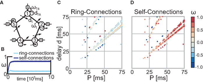
Figure 6. Stable fixed points of the ring structure (A) without noise. (B) This panel exemplifies the temporal weight development for configuration P = 70 ms and d = 58 ms. All self-connections follow practically the same temporal development and this is also true for all ring-connections. (C,D) The color code indicates the actual weight values of the fixed-points of the self-connections (C) and the ring-connections (D) dependent on the parameter P and d (delay) of the network. Parameter configurations which lead to divergent weights are not shown (i.e., are white).

Also more complex input protocols must be investigated. The current study suggest that dynamically stable recurrent sub-structures can exist within larger networks. Similar results exist for the generation of stable activity patterns in (non-plastic) networks (Memmesheimer and Timme, 2006a,b). These studies may allow us to gradually approach a better understanding of dynamically changing modular networks going beyond the currently still dominating unifying approaches, which mostly only consider feed-forward structures or randomly connected networks with average activities. This will require intensive studies but we hope that the current contribution can provide useful analytical tools and first insights into these very difficult problems.

Conflict of Interest Statement

The authors declare that the research was conducted in the absence of any commercial or financial relationships that could be construed as a potential conflict of interest.

Acknowledgment

We wish to thank M. Timme and R.-M. Memmesheimer for fruitful discussions and the German Ministry for Education and Research (BMBF) via the Bernstein Center for Computational Neuroscience (BCCN) Göttingen under Grant No. 01GQ1005A and 01GQ1005B as well as the Max Planck Society for financial support.

References

Bair, W., Koch, C., Newsome, W., and Britten, K. (1994). Power spectrum analysis of bursting cells in area MT in the behaving monkey. J. Neurosci. 74, 2870–2892.

Bi, G., and Poo, M. (1998). Synaptic modifications in cultured hippocampal neurons: dependence on spike timing, synaptic strength, and postsynaptic cell type. J. Neurosci. 18, 10464–10472.

Pubmed Abstract | Pubmed Full Text

Bienenstock, E., Cooper, L. N., and Munro, P. (1982). Theory for the development of neuron selectivity: orientation specificity and binocular interaction in visual cortex. J. Neurosci. 2, 23–48.

Burkitt, A. N., Gilson, M., and van Hemmen, J. L. (2007). Spike-timing-dependent plasticity for neurons with recurrent connections. Biol. Cybern. 96, 533–546.

Pubmed Abstract | Pubmed Full Text | CrossRef Full Text

Caporale, N., and Dan, Y. (2008). Spike-timing-dependent plasticity: a Hebbian learning rule. Annu. Rev. Neurosci. 31, 25–46.

Pubmed Abstract | Pubmed Full Text | CrossRef Full Text

Clopath, C., Büsing, L., Vasilaki, E., and Gerstner, W. (2010). Connectivity reflects coding: a model of voltage-based STDP with homeostasis. Nat. Neurosci. 13, 344–352.

Pubmed Abstract | Pubmed Full Text | CrossRef Full Text

Dayan, P., and Abbott, L. F. (2001). Theoretical Neuroscience. Cambridge, MA: MIT Press.

Deco, G., and Romo, R. (2008). The role of fluctuations in perception. Trends Neurosci. 31, 591–598.

Pubmed Abstract | Pubmed Full Text | CrossRef Full Text

Fellous, J., Rudolph, M., Destexhe, A., and Sejnowski, T. (2003). Synaptic background noise controls the input/output characteristics of single cells in an in vitro model of in vivo activity. Neuroscience 122, 811–829.

Pubmed Abstract | Pubmed Full Text | CrossRef Full Text

Ferster, D. (1988). Spatially opponent excitation and inhibition in simple cells of the cat visual cortex. J. Neurosci. 8, 1172–1180.

Pubmed Abstract | Pubmed Full Text

Gilson, M., Burkitt, A. N., Grayden, D. B., Thomas, D. A., and van Hemmen, J. L. (2009). Emergence of network structure due to spike-timing-dependent plasticity in recurrent neuronal networks iv. Biol. Cybern. 101, 427–444.

Pubmed Abstract | Pubmed Full Text | CrossRef Full Text

Gütig, R., Aharonov, R., Rotter, S., and Sompolinsky, H. (2003). Learning input correlations through nonlinear temporally asymmetric Hebbian plasticity. J. Neurosci. 23, 3697–3714.

Pubmed Abstract | Pubmed Full Text

Heeger, D. J. (1993). Modeling simple-cell direction selectivity with normalized, half-squared, linear operators. J. Neurophysiol. 70, 1885–1898.

Pubmed Abstract | Pubmed Full Text

Hopfield, J. J. (1982). Neural networks and physical systems with emergent collective computational properties. Proc. Natl. Acad. Sci. U.S.A. 79, 2554–2558.

Pubmed Abstract | Pubmed Full Text | CrossRef Full Text

Izhikevich, E. M., and Desai, N. S. (2003). Relating STDP to BCM. Neural Comput. 15, 1511–1523.

Pubmed Abstract | Pubmed Full Text | CrossRef Full Text

Izhikevich, E. M., Gally, J. A., and Edelman, G. M. (2004). Spike-timing dynamics of neuronal groups. Cereb. Cortex 14, 933–944.

Pubmed Abstract | Pubmed Full Text | CrossRef Full Text

Kempter, R., Gerstner, W., and van Hemmen, J. L. (2001). Intrinsic stabilization of output rates by spike-based Hebbian learning. Neural. Comput. 13, 2709–2741.

Pubmed Abstract | Pubmed Full Text | CrossRef Full Text

Klopf, A. H. (1988). A neuronal model of classical conditioning. Psychobiology 16, 85–123.

Kolodziejski, C., Porr, B., and Wörgötter, F. (2008). Mathematical properties of neuronal TD-rules and differential Hebbian learning: a comparison. Biol. Cybern. 98, 259–272.

Pubmed Abstract | Pubmed Full Text | CrossRef Full Text

Kosco, B. (1986). “Differential Hebbian learning,” in Neural Networks for Computing: AIP Conference Proceedings, Vol. 151, ed. J. S. Denker (New York: American Institute of Physics), 277–282.

Lubenov, E. V., and Siapas, A. G. (2008). Decoupling through synchrony in neuronal circuits with propagation delays. Neuron 58, 118–131.

Pubmed Abstract | Pubmed Full Text | CrossRef Full Text

Magee, J. C., and Johnston, D. (1997). A synaptically controlled, associative signal for Hebbian plasticity in hippocampal neurons. Science 275, 209–213.

Pubmed Abstract | Pubmed Full Text | CrossRef Full Text

Magnus, W. (1954). On the exponential solution of differential equations for a linear operator. Commun. Pure Appl. Math. VII, 649–673.

CrossRef Full Text

Markram, H., Lübke, J., Frotscher, M., and Sakmann, B. (1997). Regulation of synaptic efficacy by coincidence of postsynaptic APs and EPSPs. Science 275, 213–215.

Pubmed Abstract | Pubmed Full Text | CrossRef Full Text

Memmesheimer, R.-M., and Timme, M. (2006a). Designing complex networks. Physica D 224, 182–201.

CrossRef Full Text

Memmesheimer, R.-M., and Timme, M. (2006b). Designing the dynamics of spiking neural networks. Phys. Rev. Lett. 97, 188101.

CrossRef Full Text

Miller, K. D., and MacKay, D. J. C. (1994). The role of constraints in Hebbian learning. Neural Comput. 6, 100–126.

CrossRef Full Text

Morrison, A., Aertsen, A., and Aertsen, A. (2007). Spike-timing-dependent plasticity in balanced random networks. Neural. Comput. 19, 1437–1467.

Pubmed Abstract | Pubmed Full Text | CrossRef Full Text

Palmer, L., Jones, J., and Stepnowski, R. (1991). “Striate receptive fields as linear filters: characterization in two dimensions of space,” in The Neural Basis of Visual Function. Vision and Visual Dysfunction, Vol. 4, ed. A. G. Leventhal (Boca Raton: CRC Press), 246–265.

Pfister, J.-P., and Gerstner, W. (2006). Triplets of spikes in a model of spike timing-dependent plasticity. J. Neurosci. 26, 9673–9682.

Pubmed Abstract | Pubmed Full Text | CrossRef Full Text

Pollen, D. A., and Ronner, S. F. (1982). Spatial computation performed by simple and complex cells in the visual cortex of the cat. Vision Res. 22, 101–118.

Pubmed Abstract | Pubmed Full Text | CrossRef Full Text

Porr, B., and Wörgötter, F. (2003). Isotropic sequence order learning. Neural Comput. 15, 831–864.

Pubmed Abstract | Pubmed Full Text | CrossRef Full Text

Roberts, P. D. (1999). Computational consequences of temporally asymmetric learning rules: I. Differential Hebbian learning. J. Comput. Neurosci. 7, 235–246.

Pubmed Abstract | Pubmed Full Text | CrossRef Full Text

Roberts, P. D. (2004). Recurrent biological neuronal networks: the weak and noisy limit. Phys. Rev. E 69, 031910.

CrossRef Full Text

Roberts, P. D. (2000). Dynamics of temporal learning rules. Phys. Rev. E 62, 4077–4082.

CrossRef Full Text

Saudargiene, A., Porr, B., and Wörgötter, F. (2004). How the shape of pre- and postsynaptic signals can influence STDP: a biophysical model. Neural Comput. 16, 595–626.

Pubmed Abstract | Pubmed Full Text | CrossRef Full Text

Shadlen, M. N., and Newsome, W. T. (1998). The variable discharge of cortical neurons: implications for connectivity, computation, and information coding. J. Neurosci. 18, 3870–3896.

Pubmed Abstract | Pubmed Full Text

Song, S., Miller, K., and Abbott, L. (2000). Competitive Hebbian learning through spike-timing-dependent synaptic plasticity. Nat. Neurosci. 3, 919–926.

Pubmed Abstract | Pubmed Full Text | CrossRef Full Text

Tamosiunaite, M., Porr, B., and Wörgötter, F. (2007). Self-influencing synaptic plasticity: recurrent changes of synaptic weights can lead to specific functional properties. J. Comput. Neurosci. 23, 113–127.

Pubmed Abstract | Pubmed Full Text | CrossRef Full Text

Turrigiano, G. G., and Nelson, S. B. (2004). Homeostatic plasticity in the developing nervous system. Nat. Rev. Neurosci. 5, 97–107.

Pubmed Abstract | Pubmed Full Text | CrossRef Full Text

van Rossum, M. C. W., Bi, G. Q., and Turrigiano, G. G. (2000). Stable Hebbian learning from spike timing-dependent plasticity. J. Neurosci. 20, 8812–8821.

Pubmed Abstract | Pubmed Full Text

Wörgötter, F., Nelle, E., Li, B., Wang, L., and Diao, Y. (1998). A possible basic cortical microcircuit called “cascaded inhibition.” results from cortical network models and recording experiments from striate simple cells. Exp. Brain Res. 122, 318–332.

Pubmed Abstract | Pubmed Full Text

Wörgötter, F., and Porr, B. (2004). Temporal sequence learning, prediction, and control – a review of different models and their relation to biological mechanisms. Neural Comput. 17, 245–319.

CrossRef Full Text