Measuring neuronal branching patterns using model-based approach

Introduction

Information in the brain is processed by highly interconnected neuronal networks, where a typical cortical neuron receives signals from 1000 to 10000 neurons. To send and receive signals from such a large number of cells, neurons adopted elaborated branching structures. By tracing the extent and direction of dendrites and axons it was possible to start discovering the basic organizational principles of the brain (Ramon y Cajal, 1911; Shepherd, 2003). For instance, the apical dendrites of pyramidal cells in the cortex have an elongated shape extending through multiple cortical layers. Later it was discovered that such shape may allow pyramidal cells to constitute a functional backbone of cortical microcolumn (Mountcastle, 1957). Another example illustrating the important relationship between neuronal shape and its function comes from modeling studies. Mainen and Sejnowski (1996) illustrated how geometry of dendritic trees can affect neuronal firing pattern. Altering dendritic size or topology can even cause profound changes in firing patterns from tonic to bursting (Krichmar et al., 2002; van Ooyen et al., 2002). Thus the shape of a neuron is an important factor influencing its connectivity and function.

Considering the significance of neuronal arborization, many researchers have attempted to describe multiple aspects of neuronal geometry in a quantitative manner (for review see Uylings and van Pelt, 2002; Brown et al., 2008). The simplest measures are length and number of neuronal branches. The other frequently used measure is Sholl analysis (Sholl, 1953) which informs about distribution of dendrites as a function of distance from the soma. This is performed by counting the number of dendrite intersections for concentric circles usually centered at the cell body, of gradually increasing radius. Although Sholl analysis proved to be a sensitive measure of changes in neuronal morphology (e.g., Kolb and Whishaw, 1998; Robinson and Kolb, 2004) it cannot detect dendritic changes which do not affect somatic-centered dendritic distribution (e.g., more or less “fan-out” branching). For that reason researchers also use other measures including: distribution of segment lengths, branch diameter, branching angles, or branch order (an integer value that is incremented at every bifurcation, measuring topological distance from the soma; Smit and Uylings, 1975; Cannon et al., 1999; Uylings and van Pelt, 2002). Some measures were even invented just to quantify certain aspects of neuronal geometry, e.g., asymmetry index (Van Pelt et al., 1992). Asymmetry index is a topological measure of a tree based on the number and connectivity pattern of the segments, thus disregarding features like the length of segments, their diameters, and the spatial embedding. It ranges from 0 for perfectly symmetrical trees to one for perfectly asymmetrical trees. More recently an extension of the asymmetry index was proposed, named caulescence, which uses the weighted partition asymmetry of nodes along the main path (Brown et al., 2008). This factors out the influence of secondary subtrees and weights more heavily the bifurcations with the largest extent. Complexity of dendritic tree can also be evaluated with fractal dimension (Caserta et al., 1995; Smith et al., 1996; Soltys et al., 2001). Fractal dimension measure how “complicated” a self-similar object is, and how it fills space, as one zooms down to finer and finer scales. Nevertheless there is still no single measure which quantifies our intuitive perception of how tree-like is this shape, or how much this cell resembles a pyramidal neuron. Those simple questions are easily answered by humans but are very difficult to quantify using computers. The reason is that perception of tree-like shape requires simultaneously combining a multitude of global and local measures like spatial distribution of segments, relative lengths and direction, connectivity, symmetry, space filling, etc. To overcome this problem we propose a completely new approach: we evaluate how much “tree-like” is a neuronal shape by measuring “how easy” is to reproduce that shape by using a tree-generating algorithm.

To generate tree-like structures we used a diffusion limited aggregation (DLA) model which is especially suitable to reproduce branching structures. It was shown that this DLA-based model was able to reproduce the spatial embedding of multiple neuronal types: granule cells, Purkinje cells, pyramidal cells, and dendritic and axonal trees of interneurons (Luczak, 2006). It was achieved by changing density of diffusing particles in selected regions of space, thus increasing or decreasing branching probability of DLA as it grows through those areas. Here we show how original DLA algorithm (with uniform density of particles) could be applied to calculate “diffusiveness” of an object which intuitively could be seen as a measure of tree-like shape.

Materials and Methods

Reproducing Shape with DLA

To reproduce shape using the DLA algorithm, the position of the first particle of the future aggregate must be defined. This particle called “seed” is positioned at the origin of the object to be reproduced (Figure 1A). The growth rule for DLA can be defined inductively as follows: introduce a randomly moving particle at a large distance from an n-particle aggregate, which sticks irreversibly at its point of first contact with the aggregate, thereby forming an n + 1 particle aggregate. To reproduce shape with DLA, the above rule is modified, such that: a randomly moving particle sticks irreversibly at its point of first contact with the aggregate only if the point of that contact overlaps with a reproduced object (Figure 1B). By definition, every particle at the time of connecting to the aggregate has hit value equal to 1. Moving particles which contact the aggregate at the point not overlapping with the object are not connected (Figure 1C, particle on the right side). If such a moving particle in the next step moves to a place already occupied by the aggregate, then that particle is deleted, and the aggregate at that point registers a new hit (Figure 1D). In summary, the aggregate grows to cover the object only at the points of contact with randomly moving particles.

FIGURE 1

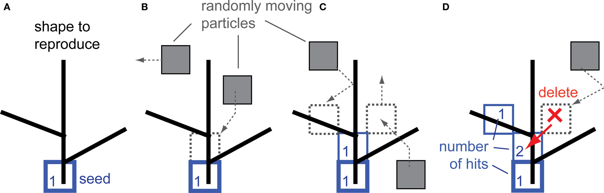
Figure 1. Reproduction of shape with the DLA algorithm. (A) The initial particle (seed) is placed as the origin of the aggregate to reproduce the given shape. (B) Randomly moving particles (gray) stick to the aggregate at the place of contact, forming new particles of the aggregate (blue). (C) Particles which contact the aggregate at places which do not overlap with the reproduced shape are not connected to the aggregate (right side particle). (D) The moving particle is deleted if it contacts the aggregate at a place which does not overlap with the reproduced shape and it moves in the next step at the place already occupied by the aggregate (red arrow). Numbers illustrate how many particles moved over (hit) that place of the aggregate – this number is called number of hits.

For computational efficiency, instead of one moving particle, m simultaneously moving particles were introduced (Voss, 1984). Also for computational simplicity, DLA was generated on a square grid, where at every iteration step, particles move by one position in the grid, in a random direction. Initially particles are uniformly distributed, with the probability of occupying a single cell in the grid set to p = 0.3. Note that although it is possible to modify the shape of DLA by changing density of diffusing particles in selected regions to produce structures resembling specific neuronal type (Luczak, 2006), here we use a uniform particle density as in the original DLA algorithm to have a generic model applicable to all cell types. The algorithm is stopped if the aggregate does not grow for 100 iterations.

The example of typical DLA is shown in Figure 2A (in gray). To reproduce this shape a seed particle is placed at the origin of the DLA, and a new DLA is grown from that point to cover it. To ensure that there are enough particles to cover the object, the area with particles is >6 times larger than that area outlined by the analyzed object. For example, in case of DLA shown in Figure 2 a grid of size 450 × 300 was used. Snapshots of the growing aggregate are shown in Figures 2A–C after 500, 1500, and 2500 iterations, respectively. In addition, in Figure 2C the position of moving particles after 2500 iterations is shown. For a typical granule cell with the total length of about 4000 μm and spanning area along x- and y-axis 400 μm × 400 μm, the size of the area with 1 μm² particles would be 3 × 400 μm × 2 × 400 μm (along x- and y-axis respectively), with probability of particle at any given point p = 0.3. Thus to cover a 4000-μm long granule cell at 1 μm resolution there is 288000 moving particles (hence 72 moving particles for every particle of the cell), which results that only a small fraction of moving particles is being used to cover typical cell.

FIGURE 2

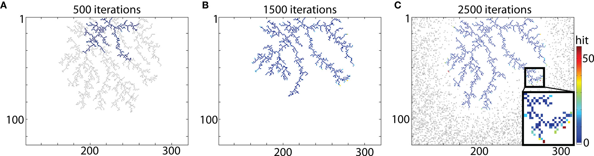
Figure 2. Reproducing DLA. (A) Growing a DLA (blue) after 500 iterations to reproduce another DLA (gray). (B) The same aggregate after 1500 iterations. (C) The same aggregate after 2500 iterations. Distribution of randomly moving particles after 2500 iterations is shown in gray. For visualization, only part with DLA is shown, the full size of grid used for that simulation was 450 × 300. Color bar on the right indicates number of hits. Note that only points on the ends of aggregate which are not growing further have exceptionally large number of hits (insert).

As explained before, a randomly moving particle after hitting the aggregate either will become a new particle of the aggregate, or will be deleted depending on whether or not the place of contact overlaps with the reproduced shape (Figure 1). To illustrate how many times a particle of the aggregate was hit by moving particles during the growth process, the aggregate is color coded for total number of hits (Figure 2; color scale shown on the right). Figure 3 illustrates the histogram of numbers of hits for an aggregate reproducing structure of typical DLA in 2D. Most of the particles in that aggregate were hit only a few times, and only a small portion of particles were hit >10 times. Importantly, the distribution of hits was very consistent across different DLAs, which is reflected in small values of SD (less than 10% of mean value; Figure 3). Note that the particles do not penetrate very deep between existing branches as particles have much higher probability to hit only the outer parts of DLA. Thus the prominent branches screen internal regions of the aggregate, preventing them from growing further which is an important feature of DLA growth algorithm (Halsey, 1997).

FIGURE 3

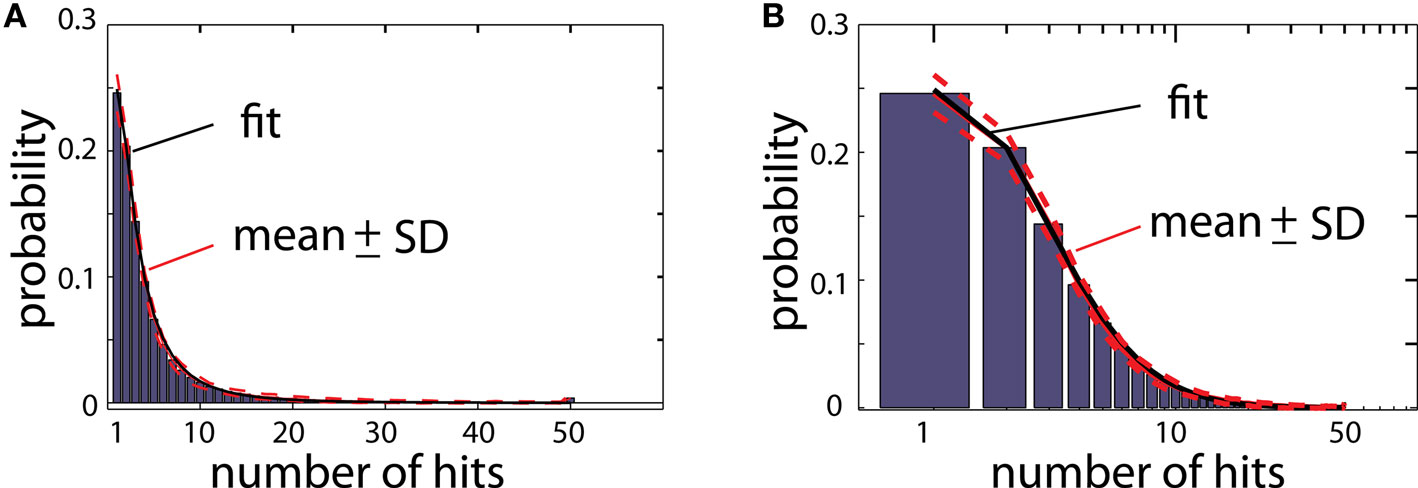
Figure 3. (A) Histogram of number of hits for an aggregate reproducing typical DLA (as in Figure 2C). For this estimate 250 DLAs were generated and reproduced. Red lines show mean value for each bin (continues line) and ±SD (dashed lines). The black line shows fit of this experimental distribution with log-normal distribution. (B) The same histogram as in (A) on logarithmic scale.

The same algorithm can also be applied to reproduce 3D shapes. In that case, particles move randomly on a 3D grid instead of 2D. An example of DLA generated in 3D is in Figure 4A. To improve visualization of 3D DLA, lines between connected particles, rather than cubic particles, are drawn. In the same figure, to help distinguish intersecting lines from different branches, the lines’ width vary depending on distance from the origin. Unfortunately, the generation of larger DLA to reproduce 3D objects at a fine scale, not only poses a challenge with visualization but also with computer memory. For example, reproducing at 1 μm resolution granule cell which can span 400 μm × 400 μm × 400 μm requires >2 GB of memory.

FIGURE 4

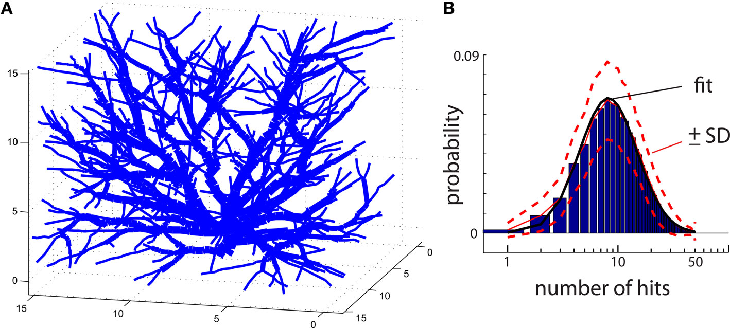
Figure 4. (A) An example of a DLA generated in 3D. To facilitate visualization only lines connecting centers of particles are shown. To distinguish intersecting lines from separate branches, the lines are assigned different width reflecting distance from the center of the aggregate. (B) Histogram of number of hits for an aggregate reproducing typical 3D DLA (as in A). Red lines show mean value (continues line) and ±SD (dashed lines). The black line shows fit of this experimental distribution with log-normal distribution plotted on logarithmic scale.

Shape Diffusion Index

The distribution of number of hits as shown in Figure 3 is characteristic for 2D DLAs. Reproduction of other types of shapes results in significantly different hit distributions which will be analyzed in more detail in the Results section. Therefore the distance between distribution of hits for DLA and distribution of hits for other shapes is a reliable measure for how DLA-like (“diffusive”) is a given shape.

Interestingly, the distribution of hits for DLA could be well approximated by log-normal distribution: where x = 1, 2,..., 50 is the number of hits and μ = 1, σ = 0.96 for 2D DLA (Figure 3), and μ = 2.46, σ = 0.6 for 3D DLA (Figure 4B). In the range of interest between 1 and 50 hits, the divergence of fit from the mean of experimentally measured distribution is always smaller than 1 SD (Figure 3). This parameterization will allow for a simpler comparison between hit distribution of DLA and hit distribution of analyzed shape. The distance between both distributions is defined as where |…| denote absolute value, d is hit distribution of analyzed shape, and <…> denote normalization to unit area (log-normal distribution has already unit area on the interval 0-inf, but because here we use interval 1–50 the area is slightly lower and such normalization improves fit for DLA). Thus for shape similar to DLA, the value of D will be close to 0, and will increase for more dissimilar shapes.

To express “diffusiveness” of an object, as measured with D, on a simple scale between 0 and 1 we propose to introduce shape diffusion index (SDI), which will be 1 for DLA-like shapes and will decrease toward 0 for less “diffusive” shapes. For that SDI is defined as SDI = exp(–D). (Matlab code is available at author’s website).

Real Neuron Morphology Data

Files with intracellularly labeled, reconstructed, and digitalized neurons were obtained from the Duke-Southampton on-line archive of neuronal morphology (http://neuron.duke.edu/cells/cellArchive.html; Cannon et al., 1998). For this analysis, the following groups of neurons were used: 38 granule cells from rat dentate gyrus, 55 CA1 hippocampal pyramidal cells stained with biocytin in whole anesthetized rats (Pyapali and Turner, 1994, 1996; Turner et al., 1995; Pyapali et al., 1998), 13 interneurons from rat dentate gyrus in brain slices stained with biocytin (Mott et al., 1997), and three Purkinje cells from the cerebellar cortex of adult guinea pigs, labeled with horseradish peroxidase, and completely reconstructed from serial sections (Rapp et al., 1994; downloaded from http://www.krasnow.gmu.edu/ascoli/CNG, Ascoli et al., 2001). For 2D analyses of neurons, values along z-axis were set to 0. The choice of diverse neuronal samples enabled the testing of SDI’s general applicability to analyze a variety of cell types.

Results

Shape Diffusion Index for Sample Objects

To illustrate values of SDI for different 2D objects we investigated a branching structure, square, and line (Figure 5). As expected, SDI was closest to 1 for the branching structure (SDI = 0.79 ± 0.04; mean ± SD; Figure 5A), and its distribution of hits (Figure 5B) was very similar as for DLA (Figure 3B). Note that not entire shape is covered (black points in Figure 5A show places with zero hits) after the end condition is reached for DLA algorithm (stop if no further growth for 100 iterations). This is because if a point is not reproduced when DLA is first growing through this area then later other branches will screen moving particles from ever reaching this point. If the point which was missed to be reproduced was at the beginning of a branch then the entire branch could not be reproduced, if this point was its only connection to the aggregate. Fortunately often in practice, to correctly estimate SDI it does not matter if part of a shape is not reproduced. This is because usually statistical properties of one part of an object are similar to other parts of that object. Thus missing one of multiple similar branches has little effect on distribution of hits. The other solution to this problem would be to estimate SDI multiple times for the same object and report average SDI. Because DLA relies on stochastic process, different parts of a shape will be reproduced or missed at each run of the algorithm. Usually repeating the SDI calculation results in a spread of SDI values within ±5%. The consistency of the results is shown in Figures 5B,D,F, where dashed lines represent ±1 SD calculated from 50 repetitions of the algorithm for the same object.

FIGURE 5

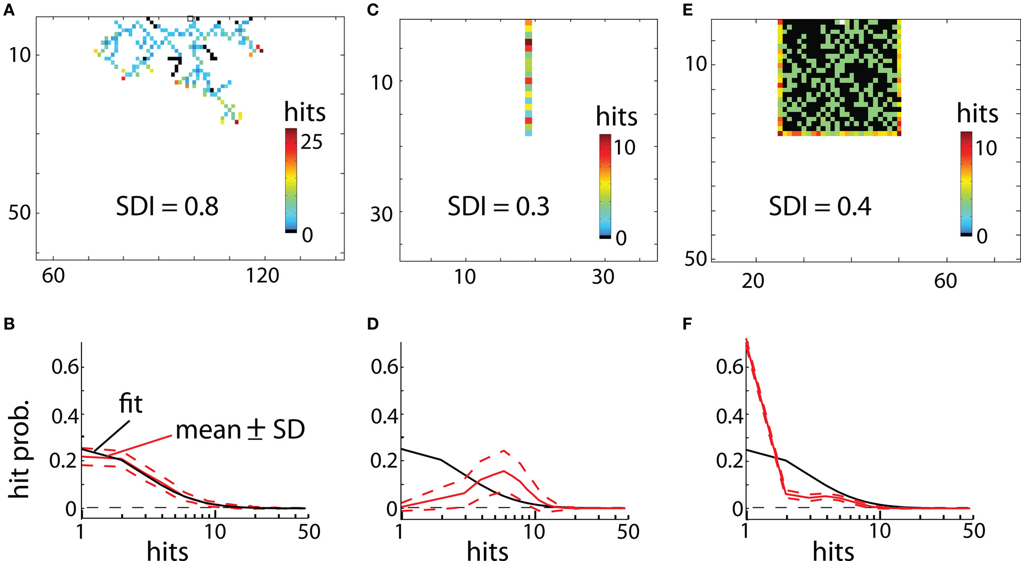
Figure 5. Examples of reproducing different shapes with DLA algorithm in 2D. (A) Reproducing branching structure. Black points indicate points of original shape which are not covered after the algorithm was terminated. Full size of grid used for that simulation was 300 × 150. (B) Hit distribution for shape in (A). Red lines indicate mean and ±SD from 50 reproductions of that shape. Black line shows fit of DLA distribution (the same as in Figure 3B). The x-axis is plotted below 0 to visualize logarithmic distribution of scale ticks (0 is indicated by horizontal dashed line). The good match between fit and this distribution indicates high diffusiveness of this shape. (C,D) Reproducing line and corresponding hit distribution. Because every particle of the line is at the border of that shape, thus each particle of line receives a large number of hits. (E) Reproducing solid square, and corresponding hit distribution in (F). Note that initially every new particle is connected to the aggregate due to overlap with the square, this results in a disproportionally large number of single hits as compared to DLA (first bin in F).

Reproducing line results in much lower values of SDI (SDI = 0.29 ± 0.04). Due to lack of screening from other branches, all parts of the line are hit by particles (Figure 5C). As opposed to DLA, the earlier covered parts of a line receive more hits than the outermost parts due to longer exposure. Therefore the hit distribution for the line is heavily skewed toward the right side (Figure 5D).

For solid shapes like a square in Figure 5E, the SDI is also significantly lower (SDI = 0.4 ± 0.012) as compared with DLA. Initially every particle hitting the aggregate becomes part of aggregate, as all connecting particles overlap with the object. For that the aggregate grows fast until it reaches the border of the square. Note that DLA cannot fill out completely solid shapes as growing branches prevent other particles from filling gaps. The distribution of hits for solid objects is composed of two parts (Figure 5F). It reflects large number of hits for points at the object border (right side of distribution), and usually a single hit for particles inside of the square (left side of distribution). Similarly, for reconstructions of objects in 3D, the highest values of SDI were obtained for 3D branching structure (SDI = 0.69 ± 0.1) and much lower values for line (SDI = 0.28 ± 0.4) and for cube (SDI = 0.26 ± 0.3).

Scale

For example, studying an oak tree at scales of millimeters is appropriate to investigate shape of a leaf or bark patterns, but to study branching patterns of a tree, the scale of meters is more suitable. In the same way a given object may be shaped by diffusive-like processes only at a particular scale. Therefore it is important to investigate the shape diffusiveness at different spatial scales. To measure at what spatial resolution a given object is, the most similar to the DLA shape a SDI can be calculated for different sizes of particles creating aggregate. For computational convenience, instead of increasing size of moving particles in relation to the reproduced object, the size of the object can be decreased, while keeping particle size the same. An example of SDI for a DLA at different scales is shown in Figure 6. Note that as spatial resolution of DLA decreases SDI changes from 0.9 to 0.45 approaching value typical for a solid object (Figures 6A–C). Similarly, when particle size become very small, multiple particle are needed to cover any “pixel” of the reproduced shape as it would be collection of solid objects, which also reduces SDI (Figure 6D).

FIGURE 6

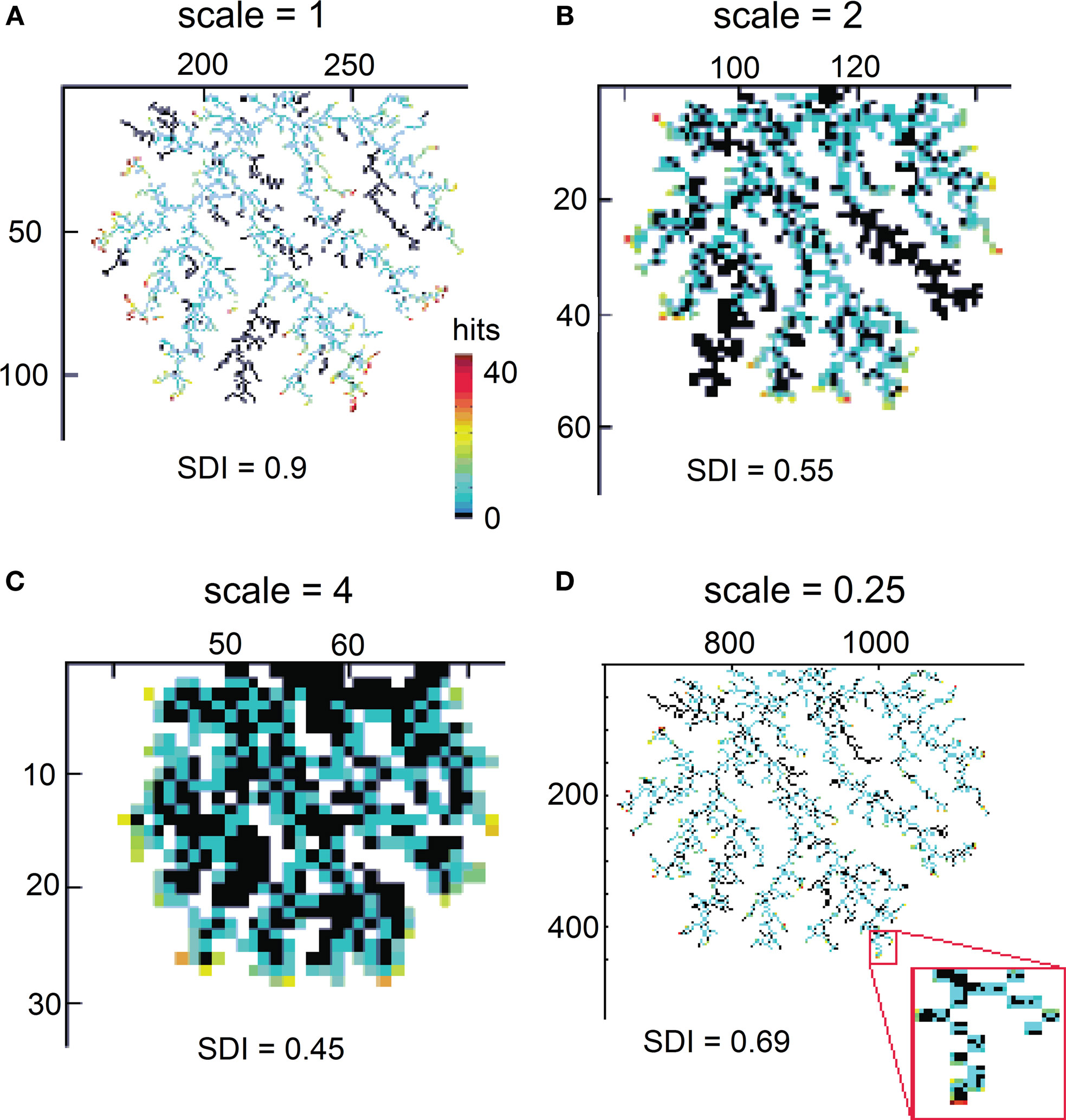
Figure 6. Reproducing an object at different scales. (A) Reproducing DLA at the scale at which it was generated. (B) Reproducing the same DLA as in (A) at twice smaller spatial resolution. (C) The same as (A) at four times smaller resolution. Full size of grid used for those simulations was 450 × 300, 225 × 150, and 112 × 75 respectively. (D) Reproducing DLA at four-times higher spatial resolution. Note in the insert that in this case multiple moving particles are required to fill one particle of DLA.

Neurons – Analysis in 2D

To evaluate diffusiveness of neuronal shape we analyzed dendritic trees of four different neuronal types: pyramidal cells, interneurons, Purkinje cells, and granule cells (Figure 7). The seed particle was located at the cell body of the reproduced neuron. This allowed generated DLA to grow in outward directions as actual neuronal processes. To investigate the scale at which a given neuron can be best reproduced with DLA models, different particle sizes were used: 1, 2, 4, 8, 16, and 32 μm.

FIGURE 7

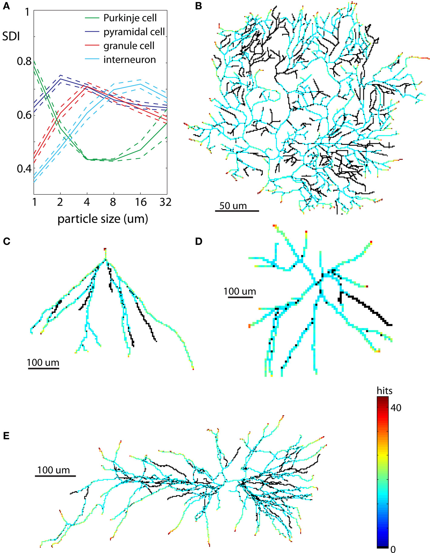
Figure 7. Examples of neurons reproduced in 2D. Each neuron is illustrated at spatial scales giving the largest SDI for that cell type. (A) Values of SDI for different types of neurons at different spatial scales (blue – pyramidal cell, green – Purkinje cell, red – granule cell, cyan – interneuron). Dashed line shows ±SEM. (B) Purkinje cell. (C) Granule cell. (D) Dendritic tree of interneuron. (E) Pyramidal cell.

The values of SDI across scales and neuronal types are summarized in Figure 7A. The spatial scale for which given cell type has the highest mean SDI indicates resolution at which it has most diffusive shape, or more precisely, resolution at which it is the most similar to DLA. Among all analyzed neurons the most diffusive shape showed Purkinje cells SDI = 0.78 ± 0.03 (mean ± SEM) at the scale of 1 μm (Figures 7A,B). At larger scales, SDI for Purkinje cells was significantly smaller. Pyramidal neurons showed the highest SDI = 0.74 ± 0.06 at the scale of 2 μm (Figures 7A,E), which was gradually decreasing for larger scales. When analyzed separately, apical dendrites usually had higher SDI than basal dendrites (SDI_apic = 0.73 ± 0.06, SDI_bas = 0.62 ± 0.06 at 2 μm). Dendritic trees of granule cells have much simpler shapes as compared to Purkinje cells or pyramidal neurons, and only at more coarse scales did granule cells resemble DLA. Thus as expected, values of SDI for granule cells were lower, and the maximum SDI = 0.71 ± 0.07 was at larger spatial scale of 4 μm; (Figures 7A,C). Interneurons had similar values of SDI as granule cells, but shifted to even larger spatial scales (maximum SDI = 0.71 ± 0.06 for 16 μm, Figures 7A,D).

Although measuring diffusiveness of a shape provides new and interesting information per se, in practice usefulness of such a measure depends on how well it can detect meaningful shape differences among analyzed neurons. To test such defined usefulness of SDI for neuroanatomical analyses, we used this measure to discriminate among different neuronal types. Each neuron was characterized by six numbers corresponding to SDI values calculated at scales: 1, 2, 4, 8, 16, and 32 μm. Using a linear discriminant analysis (Hastie et al., 2001) resulted in a well above chance discrimination among four neuronal types with 86% of neurons correctly classified (chance level is 25%). Result are summarized in Table 1. To avoid overfitting, the classifier was trained using all neurons except the predicted cell (leave-one-out cross-validation). Using non-linear methods like quadratic discriminant analysis or k-nearest neighbor classifier resulted in only minor improvement (87% correctly classified neurons). Even though an 87% success rate may not look too impressive, it compares favorably with other neuronal measures. For example, Cannon et al. (1999) used 31 different measures to quantitatively characterize 4 groups of neurons: granule cells, interneurons, and pyramidal cells from CA1 and CA3 regions. No single measure was significantly different for all pair-wise comparisons between groups (p < 0.001; Kolmogorov–Smirnov test), and only 2 out of 31 measures were significantly different between cells types used here: granule cells, interneurons and CA1 pyramidal cells (those two measures evaluate distribution of mass along principal axes: Vm₁ and Cmx; p < 0.001; Cannon et al., 1999). To compare those results more directly with SDI a first principal component was calculated to reduce vector of six SDI values describing each neuron to just one number (pc1). Using Kolmogorov–Smirnov test, distribution of pc1 values was significantly different (p < 0.0001) between analyzed here groups of granule cells, interneurons and CA1 pyramidal cells. Thus those analyses show that despite large variability of neuronal shapes, SDI can be used for reliable discrimination among cell classes, giving better results than most other neuroanatomical measures.

TABLE 1

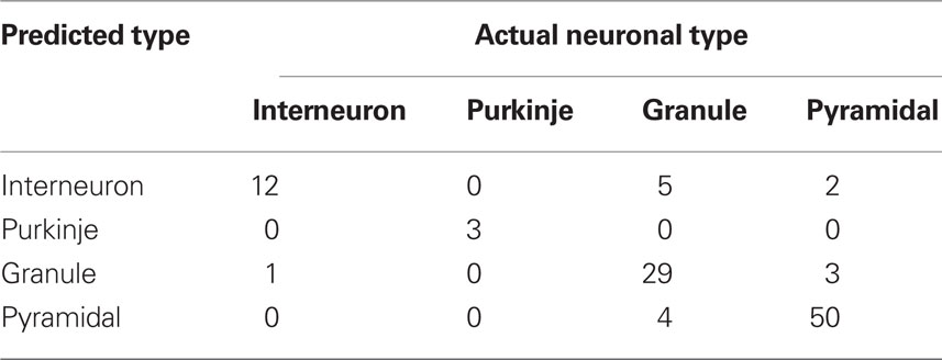
Table 1. Results of discrimination among neuronal classes using SDI calculated in 2D (linear discriminant analysis).

Neurons – Analysis in 3D

Neurons have elaborate 3D shapes, so while analyses in 2D are good for method development and an initial assessment, they may not give accurate reflection of 3D embedding. For that reason we repeated calculations of SDI for the same cells in 3D. Due to exponentially larger computational time and the computer memory demands required to generate DLA in 3D, neurons were analyzed only at five spatial scales (2, 4, 8, 16, and 32 μm). The results for all neuronal types are summarized in Figure 8A. Similarly to 2D analyses, Purkinje cells showed increasingly higher SDI for smaller scales. Other cells also show results consistent with 2D analyses with the highest SDI values at the intermediate scales. Nevertheless values of SDI for 3D neurons could not be directly derived from 2D SDI. The main difference between reproducing 2D and 3D shapes with DLA is in the larger penetrability of moving particles in 3D. For example for neurons projected to 2D the most outer parts effectively screen inner parts of dendritic tree, which causes a disproportionally large number of hits for outer parts (Figures 7B–E). In contrast, in 3D due to the additional degree of freedom (z-axis) particles can avoid more easily outer parts and reach inner branches (Figures 8B–E). This results in significantly different distribution of hits for branching shapes in 2D and 3D as shown in case of DLA in Figures 3 and 4B. Despite whose differences neuronal types could be differentiated with SDI measured in 2D with similar accuracy as in 3D. Using linear discriminant analysis as described before showed that 83% of neurons were correctly classified (chance level is 25%; Table 2).

FIGURE 8

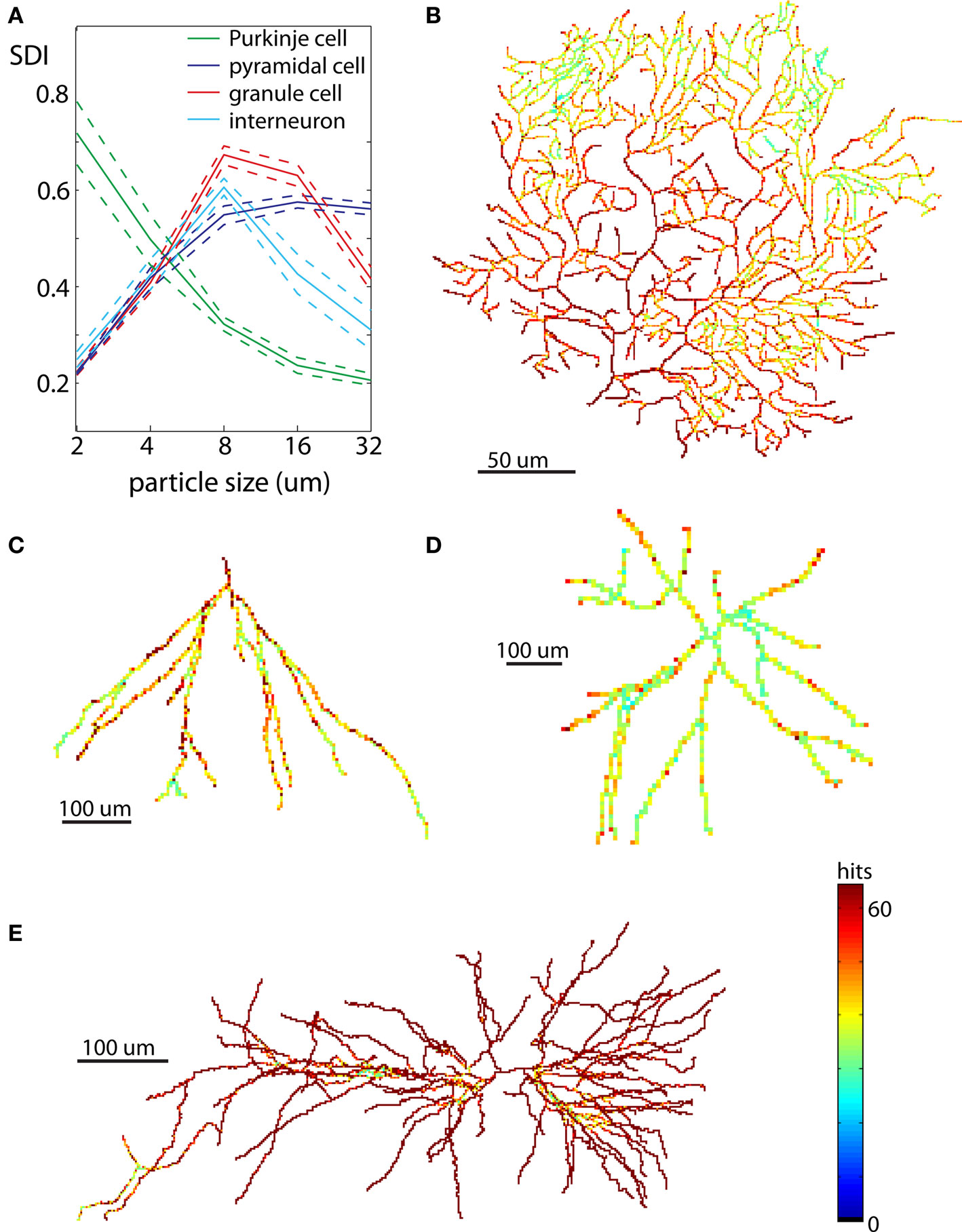
Figure 8. Examples of neurons reproduced in 3D. Each neuron is illustrated at the same scale as in Figure 7 to facilitate a comparison of spatial distribution of hits between neurons reproduced in 2D and 3D. (A) Values of SDI for different types of neurons at different spatial scales (blue – pyramidal cell, green – Purkinje cell, red – granule cell, cyan – interneuron). Dashed line shows ±SEM. (B) Purkinje cell. (C) Granule cell. (D) Dendritic tree of interneuron. (E) Pyramidal cell.

TABLE 2

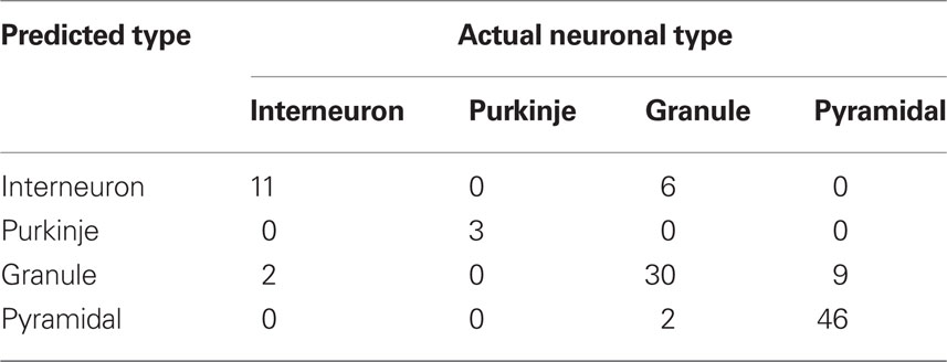
Table 2. Results of discrimination among neuronal classes using SDI calculated in 3D (linear discriminant analysis).

Discussion

In this paper we propose a Diffusion Limited Aggregate model as a “benchmark” for “diffusive” shape. Although DLA grows by connecting particles diffusing in space, DLA can also be seen as diffusing into space, where dendrites have the highest probability of growing in the direction of the largest local concentration of “trophic” particles. As a result, DLA forms complex tree-like shapes. Note that the seemingly simple concept of “tree-like shape” is in fact very difficult to quantitatively describe. For example, we would consider as a tree only a shape with a particular type of connectivity pattern, and with particular spatial distribution of segments, branching angles, relative lengths, orientation, etc. By using the DLA model to reproduce analyzed objects, we can quantify the tree-like resemblance of an object by simply measuring performance of the DLA algorithm. Thus this approach presents a conceptual change where the use a computational model allows to assess complex properties of an object, which otherwise would be very difficult to quantify with any other existing measures.

Measuring Diffusiveness

In general there is no single best measure to evaluate similarities between two objects or even graphs (Loncaric, 1998; Pelillo et al., 1998; Veltkamp and Hagedoorn, 1999; Osada et al., 2002). For that reason, generally, classifying objects into categories (e.g. car, animal, table, stool, etc.) remains still an unsolved problem in computer science (Rui et al., 1997). Thus the question of how to measure the similarity of a given shape to DLA is difficult to answer. The standard approach to this problem would be to measure: branching patterns including branching directions and angles, spatial extent of pattern in multiple directions, lengths and curvatures of branch segments, etc. Because so many different global and local measures would be necessary to extract and compare with DLA shape, this approach seems difficult to implement successfully. Here we propose a different solution: we use the DLA algorithm and measure its performance in reproducing a given pattern.

Performance of DLA algorithms could be measured in variety of ways, e.g.: how quickly it can cover shape; how completely it covers; how broad is the distribution of hits, etc. From all of the different measures we tried, the distance to the hit distribution of DLA provided the most reliable measure of similarity to DLA-like shapes. Because it is not convenient to use a distribution which is described with >50 numbers (probability for each hit values) we tried to fit the hit distribution of DLA with variety of known functions. We found a log-normal distribution to be well fitting all parts of the experimental distribution for 2D and 3D analyses. It is not obvious why a log-normal distribution, which describes the multiplicative product of many independent random variables, would be the best here, but the analytical investigation of the exact formula for the hit distribution of DLA and its relation to log-normal distribution is beyond the scope of this paper. Likely, part of the explanation is that the outermost parts of the aggregate have exponentially higher probability of being hit by randomly moving particles than the more inner parts of aggregate.

As explained in the Methods section, the hit distribution is calculated for range of hits 1–50. Nevertheless in some cases there are also parts of the reproduced shape which were never hit by diffusing particle (for example see area marked in black in Figures 5A,E or Figures 6A–D). Although the number of points with 0 hits is also informative about shape diffusiveness, it was not included in the calculation of SDI due to the high variation in number of zero hits across similar objects and even for repeated analyses of the same object. For example, if by chance the initial part of a branch was not hit by any particle then the entire branch would have zero hits (e.g., Figure 6B, right-middle branch). In another simulation, this branch could be completely cover with hits, resulting in a large variability of size of area with zero hits. On the other hand, for branches covered with hits the relative number of particles with 1–50 hits was very stable as illustrated in Figure 3 where SD is closely following the mean. Fortunately, for objects like neurons where branches are similar to each other, missing a branch or its parts had little effect on SDI which could be reliably evaluated only from covered branches. In practice this problem in only limited to 2D shapes. For neurons in 3D, particles more freely penetrate dendritic trees resulting in almost always complete coverage of neurons (compare color-coded distribution of hits in Figures 7B–E and Figures 8B–E).

Relation to Other Measures

Shape diffusiveness index is a complex measure which cannot be easily expressed with an equation. Instead SDI is defined based on hit distribution resulted from a probabilistic, iterative algorithm. SDI also cannot be directly related to a simple measure like mean segment lengths, because SDI depends on a non-trivial combination of a variety of parameters like relative spatial distribution of segments, connectivity pattern, branching angles, etc. Another difficulty with relating SDI to other measures is its non-monotonic dependence on spatial resolution, which allows the investigation of the spatial scale for branching processes. For example, for a granule cell, as shown in Figure 7A (red line), initially with the increasing spatial scale the value of SDI is also increasing, but when further increasing spatial scale above 4 μm, SDI is decreasing. Similarly, SDI cannot be directly related to more complex measures like fractal dimension, which unlike SDI, monotonically increases for more solid objects. That SDI is not easily related to other measures is also another reflection that with the current measures it would be difficult to quantify the similarity of an object to DLA.

Calculating SDI at multiple scales proved to be a reliable measure to discriminate neuronal types (Tables 1 and 2). Nevertheless at a single spatial scale, SDI may fail to differentiate between neuronal types (for instance see Figure 7A at scale of 4 μm where SDI values of pyramidal cells and granule cells highly overlap). Furthermore some trees may be a mixture of different types of branching structures (e.g., dendritic and axonal tree of a neuron) and without separating them, SDI may not provide accurate results. As mentioned earlier, it is important to remember that every measure has its limitations, SDI including.

Future Directions

Shape diffusiveness index seems to be in good agreement with an intuitive assessment of the similarity between an analyzed shape and DLA. Nevertheless, what is really needed is a measure of similarity not to an artificial structure, but to a specific type of shape. For example, it would be beneficial to have a measure describing if a particular neuron looks like a normal and healthy Purkinje cell. For instance, such a measure would be of interest when screening for irregularities in dendritic morphology caused by disease, drug, and/or aging. To achieve this, an approach suggested by this study would be to generate not a generic DLA model, but instead a DLA-based model of a specific neuronal type, and this tailored model would be used to reproduce an analyzed shape (modifying density of particles in space will result in DLAs resembling different neuronal types). Importantly, the method proposed here is not restricted to DLA models only. Most likely, any other model of neuronal growth could be successfully used to quantify the similarity of a given shape to, e.g., pyramidal neuron. It could be implemented in an analogous fashion to the DLA model, where by evaluating “how easy” it is to reproduce shape of a given neuron by using model proposed by Ascoli and Krichmar (2000), Samsonovich and Ascoli (2005), Eberhard et al. (2006), Koene et al. (2009), or Cuntz et al. (2010), could provide a good measure capable of competing with an experienced anatomist to quickly spot unusual neuronal trees.

Conflict of Interest Statement

The author declares that the research was conducted in the absence of any commercial or financial relationships that could be construed as a potential conflict of interest.

Acknowledgments

This work was supported by NSERC and AHFMR grants.

References

Ascoli, G., and Krichmar, J. (2000). L-neuron: a modeling tool for the efficient generation and parsimonious description of dendritic morphology. Neurocomputing 32–33, 1003–1011.

CrossRef Full Text

Ascoli, G. A., Krichmar, J., Nasuto, S., and Senft, S. (2001). Generation, description and storage of dendritic morphology data. Philos. Trans. R. Soc. Lond. B Biol. Sci. 356, 1131–1145.

Pubmed Abstract | Pubmed Full Text | CrossRef Full Text

Brown, K. M., Gillette, T. A., and Ascoli, G. A. (2008). Quantifying neuronal size: summing up trees and splitting the branch difference. Semin. Cell Dev. Biol. 19, 485–493.

Pubmed Abstract | Pubmed Full Text | CrossRef Full Text

Cannon, R. C., Turner, D. A., Pyapali, G. K., and Wheal, H. V. (1998). An on-line archive of reconstructed hippocampal neurons. J. Neurosci. Methods 84, 49–54.

Pubmed Abstract | Pubmed Full Text | CrossRef Full Text

Cannon, R. C., Wheal, H. V., and Turner, D. A. (1999). Dendrites of classes of hippocampal neurons differ in structural complexity and branching patterns. J. Comp. Neurol. 413, 619–633.

Pubmed Abstract | Pubmed Full Text | CrossRef Full Text

Caserta, F., Eldred, W. D., Fernandez, E., Hausman, R. E., Stanford, L. R., Bulderev, S. V., Schwarzer, S., and Stanley, H. E. (1995). Determination of fractal dimension of physiologically characterized neurons in two and three dimensions. J. Neurosci. Methods 56, 133–144.

Pubmed Abstract | Pubmed Full Text | CrossRef Full Text

Cuntz, H., Forstner, F., Borst, A., and Hausser, M. (2010). One rule to grow them all: a general theory of neuronal branching and its practical application. PLoS Comput. Biol. 6, e1000877. doi: 10.1371/journal.pcbi.1000877.

Pubmed Abstract | Pubmed Full Text | CrossRef Full Text

Eberhard, J. P., Wanner, A., and Wittum, G. (2006). NeuGen: a tool for the generation of realistic morphology of cortical neurons and neuronal networks in 3D. Neurocomputing 70, 327–342.

CrossRef Full Text

Halsey, T. C. (1997). The branching structure of diffusion limited aggregates. Europhys. Lett. 39, 43–48.

CrossRef Full Text

Hastie, T., Tibshirani, R., and Friedman, J. (2001). The Elements of Statistical Learning: Data Mining, Inference, and Prediction, 1st Edn. New York: Springer-Verlag.

Koene, R. A., Tijms, B., van Hees, P., Postma, F., de Ridder, A., Ramakers, G. J., van Pelt, J., and van Ooyen, A. (2009). NETMORPH: a framework for the stochastic generation of large scale neuronal networks with realistic neuron morphologies. Neuroinformatics 3, 195–210.

CrossRef Full Text

Kolb, B., Whishaw, I., and Q. (1998). Brain plasticity and behavior. Annu. Rev. Psychol. 49, 43–64.

Pubmed Abstract | Pubmed Full Text | CrossRef Full Text

Krichmar, J. L., Nasuto, S. J., Scorcioni, R., Washington, S. D., and Ascoli, G. A. (2002). Effects of dendritic morphology on CA3 pyramidal cell electrophysiology: a simulation study. Brain Res. 941, 11–28.

Pubmed Abstract | Pubmed Full Text | CrossRef Full Text

Loncaric, S. (1998). A survey of shape analysis techniques. Pattern Recognit. 31, 983–1001.

CrossRef Full Text

Luczak, A. (2006). Spatial embedding of neuronal trees modeled by diffusive growth. J. Neurosci. Methods 157, 132–141.

Pubmed Abstract | Pubmed Full Text | CrossRef Full Text

Mainen, Z. F., and Sejnowski, T. J. (1996). Influence of dendritic structure on firing pattern in model neocortical neurons. Nature 382, 363–366.

Pubmed Abstract | Pubmed Full Text | CrossRef Full Text

Mott, D. D., Turner, D. A., Okazaki, M. M., and Lewis, D. V. (1997). Interneurons of the dentate hilus border of the rat dentate gyrus: anatomical and electrophysiological heterogeneity. J. Neurosci. 17, 3990–4005.

Pubmed Abstract | Pubmed Full Text

Mountcastle, V. B. (1957). Modality and topographic properties of single neurons of cat’s somatic sensory cortex. J. Neurophysiol. 20, 408–434.

Pubmed Abstract | Pubmed Full Text

Osada, R., Funkhouser, T., Chazelle, B., and Dobkin, D. (2002). Shape distributions. ACM Trans. Graph. 21, 807–832.

CrossRef Full Text

Pelillo, M., Siddiqi, K., and Zucker, S. W. (1998). “Matching hierarchical structures using association graphs,” in Proceedings of the Fifth European Conference on Computer Vision, June 1998, Vol. II, Lecture Notes in Computer Science 1406, eds H. Burkhardt and B. Neumann (Freiburg: Springer-Verlag), 3–16.

Pyapali, G. K., Sik, A., Penttonen, M., Buzsáki, G., and Turner, D. A. (1998). Dendritic properties of hippocampal CA1 pyramidal neurons in the rat: intracellular staining in vivo and in vitro. J. Comp. Neurol. 391, 335–352.

Pubmed Abstract | Pubmed Full Text | CrossRef Full Text

Pyapali, G. K., and Turner, D. A. (1994). Denervation-induced dendritic alterations in CA1 pyramidal cells following kainic acid hippocampal lesions in rats. Brain Res. 652, 279–290.

Pubmed Abstract | Pubmed Full Text | CrossRef Full Text

Pyapali, G. K., and Turner, D. A. (1996). Increased dendritic extent in hippocampal CA1 neurons from aged F344 rats. Neurobiol. Aging 17, 601–611.

Pubmed Abstract | Pubmed Full Text | CrossRef Full Text

Ramon y Cajal, S. (1911). Histology of the Nervous System of Man and Vertebrates, Vol. 1 (Translated By L. Swanson and N. Swanson, 1995). Oxford, UK: Oxford University Press.

Rapp, M., Segev, I., and Yarom, Y. (1994). Physiology, morphology and detailed passive models of guinea-pig cerebellar Purkinje cells. J. Physiol. 474, 101–118.

Pubmed Abstract | Pubmed Full Text

Robinson, T. E., and Kolb, B. (2004). Structural plasticity associated with exposure to drugs of abuse. Neuropharmacology 47, 33–46.

Pubmed Abstract | Pubmed Full Text | CrossRef Full Text

Rui, Y., Huang, T. S., and Chang, S. F. (1997). Image retrieval: past, present, and future. J. Vis. Commun. Image Represent. 10, 1–23.

Samsonovich, A., and Ascoli G. (2005). Statistical determinants of dendritic morphology in hippocampal pyramidal neurons: a hidden Markov model. Hippocampus 15, 166–183.

Pubmed Abstract | Pubmed Full Text | CrossRef Full Text

Shepherd, G. M. (ed.). (2003). The Synaptic Organization of the Brain, 5th Edn. Oxford: Oxford University Press.

Sholl, D. A. (1953). Dendritic organization in the neurons of the visual and motor cortices of the cat. J. Anat. 87, 387–406.

Pubmed Abstract | Pubmed Full Text

Smit, G. J., and Uylings, H. B. (1975). The morphometry of the branching pattern in dendrites of the visual cortex pyramidal cells. Brain Res. 87, 41–53.

Pubmed Abstract | Pubmed Full Text | CrossRef Full Text

Smith, T. G. Jr., Lange, G. D., and Marks, W. B. (1996). Fractal methods and results in cellular morphology – dimensions, lacunarity and multifractals. J. Neurosci. Methods 69, 123–136.

Pubmed Abstract | Pubmed Full Text | CrossRef Full Text

Soltys. Z., Ziaja, M., Pawlínski, R., Setkowicz, Z., and Janeczko, K. (2001). Morphology of reactive microglia in the injured cerebral cortex. Fractal analysis and complementary quantitative methods. J. Neurosci. Res. 63, 90–97.

Pubmed Abstract | Pubmed Full Text | CrossRef Full Text

Turner, D. A., Li, X. G., Pyapali, G. K., Ylinen, A., and Buzsáki, G. (1995). Morphometric and electrical properties of reconstructed hippocampal Ca3 neurons recorded in vivo. J. Comp. Neurol. 356, 580–594.

Pubmed Abstract | Pubmed Full Text | CrossRef Full Text

Uylings, H. B., and van Pelt, J. (2002). Measures for quantifying dendritic arborizations. Network 13, 397–414.

Pubmed Abstract | Pubmed Full Text | CrossRef Full Text

van Ooyen, A., Duijnhouwer, J., Remme, M. W., and van Pelt, J. (2002), The effect of dendritic topology on firing patterns in model neurons. Network 13, 311–325.

Pubmed Abstract | Pubmed Full Text | CrossRef Full Text

Van Pelt, J., Uylings, H. B. M., Verwer, R. W. H., Pentney, R. J., and Woldenberg, M. J. (1992). Tree asymmetry – a sensitive and practical measure for binary topological trees. Bull. Math. Biol. 54:759–84

Pubmed Abstract | Pubmed Full Text

Veltkamp, R. C., and Hagedoorn, M. (1999). State-of-the-Art in Shape Matching. Technical Report UU-CS-1999-27. The Netherlands: Utrecht University.

Voss, R. F. (1984). Multiparticle fractal aggregation. J. Stat. Phys. 36, 861–872.

CrossRef Full Text