STDP in adaptive neurons gives close-to-optimal information transmission

Introduction

The experimental discovery of spike-timing-dependent plasticity (STDP) in the mid-nineties (Bell et al., 1997; Magee and Johnston, 1997; Markram et al., 1997; Bi and Poo, 1998; Zhang et al., 1998) led to two questions, in particular. The first is: what is the simplest way of describing this complex phenomenon? This question has been answered in a couple of minimal models (phenomenological approach) whereby long-term potentiation (LTP) and long-term depression (LTD) are reduced to the behavior of a small number of variables (Gerstner et al., 1996; Kempter et al., 1999; Song et al., 2000; van Rossum et al., 2000; Rubin et al., 2001; Gerstner and Kistler, 2002a; Froemke et al., 2006; Pfister and Gerstner, 2006; Clopath et al., 2010; see Morrison et al., 2008 for a review). Because they are inspired by in vitro plasticity experiments, the state variables usually depend solely on what is experimentally controlled, i.e., on spike times and possibly on the postsynaptic membrane potential. They are computationally cheap enough to be used in large-scale simulations (Morrison et al., 2007; Izhikevich and Edelman, 2008). The second question has to do with the functional role of STDP: what is STDP good for? The minimal models mentioned above can address this question only indirectly, by solving the dynamical equation of synaptic plasticity for input with given stationary properties (Kempter et al., 1999; van Rossum et al., 2000; Rubin et al., 2001). An alternative approach is to postulate a role for synaptic plasticity, and formulate it in the mathematical framework of optimization (“top-down approach”). Thus, in artificial neural networks, Hebbian-like learning rules were shown to arise from unsupervised learning paradigms such as principal components analysis (Oja, 1982, 1989), independent components analysis (ICA; Intrator and Cooper, 1992; Bell and Sejnowski, 1995; Clopath et al., 2008), maximization of mutual information (MI; Linsker, 1989), sparse coding (Olshausen and Field, 1996; Smith and Lewicki, 2006), and predictive coding (Rao and Ballard, 1999). In spiking neurons, local STDP-like learning rules were obtained from optimization criteria such as maximization of information transmission (Chechik, 2003; Toyoizumi et al., 2005, 2007), information bottleneck (Klampfl et al., 2009), maximization of the neuron’s sensitivity to the input (Bell and Parra, 2005), reduction of the conditional entropy (Bohte and Mozer, 2007), slow-feature analysis (Sprekeler et al., 2007), and maximization of the expected reward (Xie and Seung, 2004; Pfister et al., 2006; Florian, 2007; Sprekeler et al., 2009).

The functional consequences of STDP have mainly been investigated in simple integrate-and-fire neurons, where the range of temporal dependencies in the postsynaptic spike train spans no more than the membrane time constant. Few studies have addressed the question of the synergy between STDP and more complex dynamical properties on different timescales. In Seung (2003), more complex dynamics were introduced not at the cell level, but through short-term plasticity of the synapses. The postsynaptic neuron was then able to become selective to temporal order in the input. Another elegant approach to this question was taken in Lengyel et al. (2005) in a model of hippocampal autoassociative memory. Memories were encoded in the phase of firing of a population of neurons relative to an ongoing theta oscillation. Under the assumption that memories are stored using a classical form of STDP, they derived the form of the postsynaptic dynamics that would optimally achieve their recall. This turned out to match what they recorded in vitro, suggesting that STDP might optimally interact with the dynamical properties of the postsynaptic cell in this memory storage task.

More generally, optimality models are ideally suited to study plasticity and dynamics together. Indeed, optimal learning rules contain an explicit reference to the dynamical properties of the postsynaptic cell, by means of the transfer function that maps input to output values. This function usually appears in the formulation of a gradient ascent on the objective function. In this article, we exploit this in order to relate STDP to spike-frequency adaptation (SFA), an important feature of the dynamics of a number of cell types found in cortex. Recent phenomenological models of STDP have emphasized the importance of the interaction between postsynaptic spikes in the LTP process (Senn et al., 2001; Pfister and Gerstner, 2006; Clopath et al., 2010). In these models, the amount of LTP obtained from a pre-before-post spike pair increases with the number of postsynaptic spikes fired in the recent past, which we call the “triplet effect” (combination of one pre-spike and at least two post-spikes). The timescale of this post–post interaction was fitted to in vitro STDP experiments, and found to be very close to that of adaptation (100–150 ms).

We reason that STDP may be ideally tuned to SFA of the postsynaptic cell. We specifically study this idea within the framework of optimal information transmission (infomax) between input and output spike trains. We compare the performance of a learning rule derived from the infomax principle in Toyoizumi et al. (2005), to that of the triplet model developed in Pfister and Gerstner (2006). We also compare them to the standard pair-based learning window used in most STDP papers. Performance is measured in terms of information theoretic quantities. We find that the triplet learning rule yields a better performance than pair-STDP on a spatio-temporal receptive field formation task, and that this advantage crucially depends on the presence of postsynaptic SFA. This reflects a synergy between the triplet effect and adaptation. The reasons for this optimality are further studied by showing that the optimal model features a similar triplet effect when the postsynaptic neuron adapts. We also show that both the optimal and triplet learning rules increase the variability of the postsynaptic spike trains, and enlarge the frequency band in which signals are transmitted, extending it toward lower frequencies (1–5 Hz). Finally, we exploit the optimal model to predict the form of the STDP mechanism for two different target cell types. The results qualitatively agree with the in vitro data reported for excitatory synapses onto principal cells and those onto fast-spiking (FS) inhibitory interneurons. In the model, the learning windows are different because the intrinsic dynamical properties of the two postsynaptic cell types are different. This might be the functional reason for the target-cell specificity of STDP.

Materials and Methods

Neuron Model

We simulate a single stochastic point neuron (Gerstner and Kistler, 2002b) and a small portion of its incoming synapses (N = 1 for the simulation of in vitro experiments, N = 100 in the rest of the paper). Each postsynaptic potential (PSP) adds up linearly to form the total modeled synaptic drive

with

where denotes the j^th input spike train, and w_j (mV) are the synaptic weights. The effect of thousands of other synapses is not modeled explicitly, but treated as background noise. The firing activity of the neuron is entirely described by an instantaneous firing density

where

is the gain function, drawn in Figure 1A. Refractoriness and SFA both modulate the instantaneous firing rate via

The variables g_R and g_A evolve according to

where is the postsynaptic spike train and 0 < τ_R ≪ τ_A are the time constants of refractoriness and adaptation respectively. The firing rate thus becomes a compressive function of the average gain, as shown in Figure 1B. The response of the neuron to a step in input firing rate is depicted in Figure 1C.

For the simulation of in vitro STDP experiments, only one synapse is investigated. The potential u is thus given a baseline u_b (to which the PSP of the single synapse will add) such that g(u_b) yields a spontaneous firing rate of 7.5 Hz (Figure 1B).

FIGURE 1

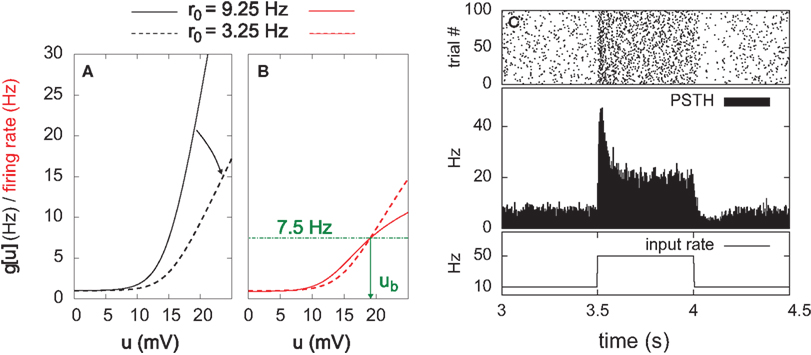
Figure 1. Stochastic neuron model. (A) The gain function g(u) (Eq. 4, solid line here) shows the momentary rate of a non-refractory neuron as a function of the membrane potential u. (B) The mean rate 〈g[u(t)]M(t)〉 of a neuron with refractoriness and adaptation is lower (solid red line). The baseline potential u_b used in the simulation is defined as the membrane potential that yields a spontaneous firing rate of 7.5 Hz (green arrow and dashed line). In some simulations, we need to switch off adaptation, but we want the same holding potential u_b to evoke the same 7.5 Hz output firing rate. The slope r₀ of the gain function is therefore rescaled (A, dashed curve) so that the frequency curves in the adaptation and no-adaptation cases (B, solid and dashed red curves) cross at u = u_b. (C) Example response property of an adaptive neuron. A single neuron receives synaptic inputs from 100 Poisson spike trains with a time-varying rate. The experiment is repeated 1000 times independently. Bottom: the input rate jumps from 10 to 50 Hz, stays there for half a second and returns back to 10 Hz (bottom). Middle: Peri-stimulus time histogram (PSTH, 4 ms bin). Top: example spike trains (first 100 trials).

In some of our simulations, postsynaptic SFA is switched off (q_A = 0). In order to preserve the same average firing rate given the same synaptic weights, r₀ is rescaled accordingly (Figures 1A,B, dashed lines).

In the simulation of Figure 8, we add a third variable g_B in the after-spike kernel M in order to model a FS inhibitory interneuron. This variable jumps down (q_B < 0) following every postsynaptic spike, and decays exponentially with time constant τ_B (with τ_R ≪ τ_B < τ_A).

All simulations were written in Objective Caml and run on a standard desktop computer operated by Linux. We used simple Euler integration of all differential equations, with 1 ms time resolution (0.1 ms for the simulation of in vitro experiments). All parameters are listed in Table 1 together with their values.

TABLE 1

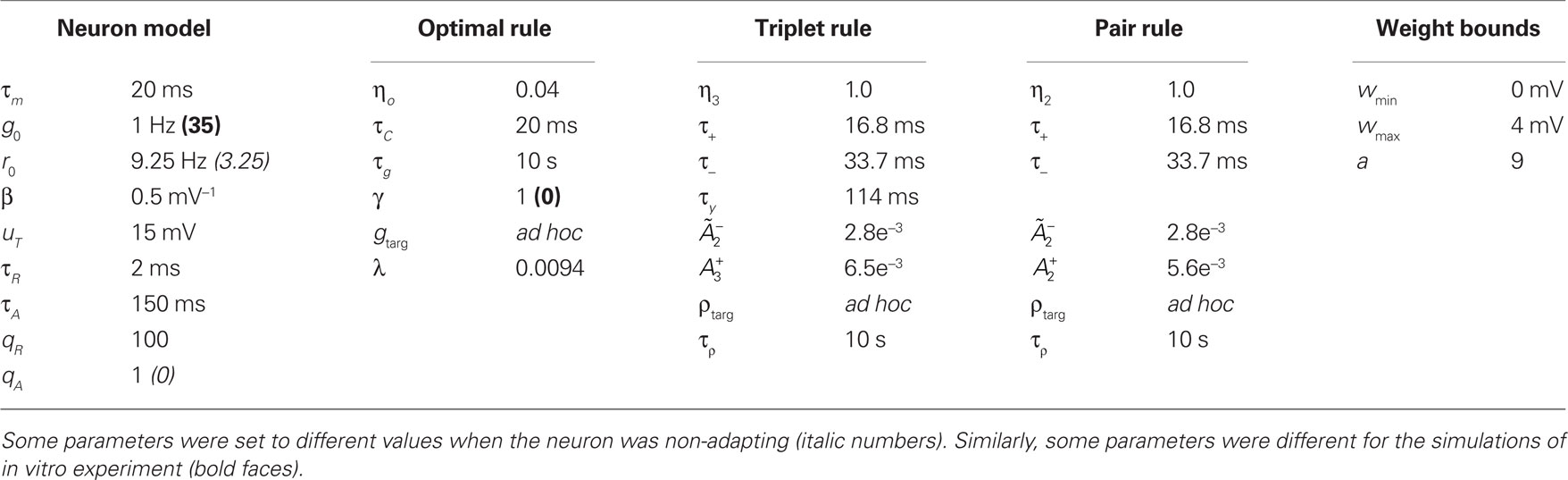
Table 1. Baseline values of all parameters defined in the text.

Presynaptic Firing Statistics

To analyze the evolution of information transmission under different plasticity learning rules, we consider N = 100 periodic input spike of 5 s duration generated once and for all (see below). This “frozen noise” is then replayed continuously, feeding the postsynaptic neuron for as long as is necessary (e.g., for learning, or for MI estimation).

To generate the time-varying rates of the N processes underlying this frozen noise, we first draw point events at a constant Poisson rate of 10 Hz, and then smooth them with a Gaussian kernel of width 150 ms. Rates are further multiplicatively normalized so that each presynaptic neuron fires an average of 10 spikes per second. We emphasize that this process describes the statistics of the inputs across different learning experiments. When we mention “independent trials,” we mean a set of experiments which have their own independent realizations of those input spike trains. However, in one learning experiment, a single such set of N input spike trains is chosen and replayed continuously as input to the postsynaptic neuron. The input is therefore deterministic and periodic. When the periodic input is generated, some neurons can happen to fire at some point during those 5 s within a few milliseconds of each other, and by virtue of the periodicity, these synchronous firing events will repeat in each period, giving rise to strong spatio-temporal correlations in the inputs. We are interested in seeing how different learning rules can exploit this correlational structure to improve the information carried by the postsynaptic activity about those presynaptic spike trains. We now describe what we mean by information transmission under this specific stimulation scenario.

Information Theoretic Measurements

The neuron can be seen as a noisy communication channel in which multidimensional signals are compressed and distorted before being transmitted to subsequent receivers. The goodness of a communication channel is traditionally measured by Shannon’s MI between the input and output variables, where the input is chosen randomly from some “alphabet” or vocabulary of symbols.

Here, the input is deterministic and periodic (Figure 2A). We therefore define the quality of information transmission by the reduction of uncertainty about the phase of the current input if we observe a certain output spike train at an unknown time. In discrete time (with time bin Δ = 1 ms), there are only N_φ = 5000 possible phases since the input has a period of 5 s. Therefore, the maximum number of bits that the noisy postsynaptic neuron can transmit is log₂(N_φ) ≃ 12.3 bits. We further assume that an observer of the output neuron can only see “words” corresponding to spike trains of finite duration T = KΔ. We assume T = 1 s for most of the paper, which corresponds to K = 1000 time bins. This choice is justified below.

FIGURE 2

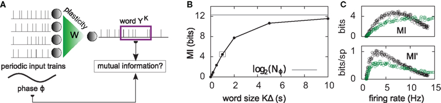
Figure 2. Information transmission through a noisy postsynaptic neuron. (A) Schematic representation of the feed-forward network. Five-second input spike trains repeat continuously in time (periodic input) and drive a noisy and possibly adapting output neuron via plastic synapses. It is assumed that an observer of the output spike train has access to portions Y^K of it, called “words,” of duration T = KΔ. The observer does not have access to a clock, and therefore has a flat prior expectation over possible phases before observing a word. The goodness of the system, given a set of synaptic weights w, is measured by the reduction of uncertainty about the phase, gained from the observation of an output word Y^K (mutual information, see text). (B) For a random set of synaptic weights (20 weights at 4 mV, the rest at 0), the mutual information (MI) is reported as a function of the output word size KΔ. Asymptotically, the MI converges to the theoretical limit given by log₂(N_φ) ( 12.3 bits. In the rest of this study, 1-s output words are considered (square). (C) Mutual information (MI, top) and information per spike (MI’, bottom) as a function of the average firing rate. Black: with SFA. Green: without SFA. Each dot is obtained by setting a fraction of randomly chosen synaptic efficacies to the upper bound (4 mV) and the rest to 0. The higher the fraction of non-zero weights, the higher the firing rate. The information per spike is a relevant quantity because spike generation costs energy.

The discretized output spike trains of size K (binary vectors), called Y^K, can be observed at random times and play the role of the output variable. The input random variable is the phase φ of the input. The quality of information transmission is quantified by the MI, i.e., the difference between the total response entropy and the noise entropy Here 〈•〉 denotes the ensemble average. In order to compute these entropies, we need to be able to estimate the probability of occurrence of any sample word Y^K, knowing and not knowing the phase. To do so, a large amount of data is first generated. The noisy neuron is fed continuously for a large number of periods N_p = 100 with a single periodic set of input spike trains and a fixed set of synaptic weights. The output spikes are recorded with Δ = 1 ms precision. From this very long output spike train, we randomly pick words of length K and gather them in a set 𝒮. We take |𝒮| = 1000. This is our sample data.

In general, estimating the probability of a random binary vector of size K is very difficult if K is large. Luckily, we have a statistical model for how spike trains are generated (Eq. 3), which considerably reduces the amount of data needed to produce a good estimate. Specifically, if the refractory state of the neuron [g_R(t),g_A(t)] is known at time t (initial conditions), then the probability 1 − exp(−ρ_kΔ) ≃ ρ_kΔ of the postsynaptic neuron spiking is also known for each of the K time bins following t (Eqs 3–5). The neuron model gives us the probability that a word Y^K occurred at time t – not necessarily the time at which the word was actually picked – (Toyoizumi et al., 2005):

where ρ_k = ρ(t + kΔ) and is one if there is a spike in the word at position k, and 0 otherwise. To compute the conditional probability of occurrence of a word Y^K knowing the phase φ, we have to further average Eq. 7:

where φ(t) = 1 + (t mod N_φ) denotes the phase at time t. Averaging over multiple times with same phase also averages over the initial conditions [g_R(t),g_A(t)], so that they do not appear in Eq. 8. The average in Eq. 8 is estimated using a set of 10 randomly chosen times t_i with φ(t_i) = φ.

The full probability of observing a word Y^K is given by where P(Y^K | φ) is computed as described above. Owing to the knowledge of the model that underlies spike generation, and to this huge averaging over all the possible phases, the obtained P(Y^K) is a very good estimate of the true density. We can then take a Monte-Carlo approach to estimate the entropies, using the set 𝒮 of randomly picked words: can be estimated by

and is estimated using

The MI estimate is the difference of these two entropies, and is expressed in bits. In Figure 2C, we introduce the information per spike MI’ (bits/spike), obtained by dividing the MI by the expected number of spikes in a window of duration KΔ. Figure 2B shows that the MI approaches its upper bound log₂(N_φ) as the word size increases. The word size considered here (1 s) is large enough to capture the effects of SFA while being small enough not to saturate the bound.

Although we constrain the postsynaptic firing rate to lie around a fixed value ρ_targ (see homeostasis in the next section), the rate will always jitter. Even a small jitter of less than 0.5 Hz (which we have in the present case) makes it impossible to directly compare entropies across learning rules. Indeed, while the MI depends only weakly on small deviations of the firing rate around ρ_targ, the response and noise entropies have much larger (co-)variations. In order to compare the entropies across learning rules, we need to know what the entropy would have been if the rate was exactly ρ_targ instead of ρ_targ + ε. We therefore compute the entropy [H(Y^K) or H(Y^K|φ)] for different firing rates in the vicinity of ρ_targ. These firing rates are achieved by slightly rescaling the synaptic weights, i.e., w_ij ← κw_ij where κ takes several values around 1. We then fit a linear model H = aρ + b, and evaluate H at ρ_targ.

The computation of the conditional probabilities P(Y^K|φ) was accelerated on an ATI Radeon (HD 4850) graphics processing unit (GPU), which was 130 times faster than a decent CPU implementation.

Learning Rules

Optimal learning rule

The optimal learning rule aims at maximizing information transmission under some metabolic constraints (“infomax” principle). Toyoizumi et al. (2005, 2007) showed that this can be achieved by means of a stochastic gradient ascent on the following objective function

whereby the mutual information 𝕀 between input and output spike trains competes with a homeostatic constraint on the mean firing rate 𝔻 and a metabolic penalty Ψ for strong weights that are often active. The first constraint is formulated as where KL denotes the Kullback–Leibler (KL) divergence. P denotes the true probability distribution of output spike trains produced by the stochastic neuron model, while assumes a similar model in which the gain g(t) is kept constant at a target gain g_targ. Minimizing the divergence between P and therefore means driving the average gain close to g_targ, thus implementing firing rate homeostasis. The second constraint reads whereby the cost for synapse j is proportional to its weight w_j and to the average number n_j of presynaptic spikes relayed during the K time bins under consideration. The Lagrange multipliers γ and λ set the relative importance of the three objectives.

Performing gradient ascent on 𝕃 yields the following online learning rule (Toyoizumi et al., 2005, 2007):

where

and

η_o is a small learning rate. The first term C_j is Hebbian in the sense that it reflects the correlations between the input and output spike trains. B_post is purely postsynaptic: it compares the instantaneous gain g to its average (information term), as well as the average gain to its target value g_targ (homeostasis). The average is estimated online by a low pass filter of g with time constant τ_g. The time course of these quantities is shown in Figure 3A for example spike trains of 1 s duration, for γ = 0.

FIGURE 3

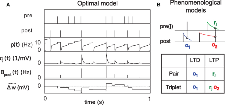
Figure 3. Description of the three learning rules. (A) Time course of the variables involved in the optimal model. denotes the cumulative weight change. (B) Schematic representation of the phenomenological models of STDP used in this paper. Each presynaptic spike yields LTD proportionally to o₁ (blue trace) in both models (pair and triplet). In the pair model, postsynaptic spikes evoke LTP proportionally to r_j (green trace), while in the triplet model r_j is combined with an additional postsynaptic trace o₂ (red).

Because of the competition between the three objectives in Eq. 11, the homeostatic constraint does not yield the exact desired gain g_targ. In practice, we set the value of g_targ empirically, such that the actual mean firing rate approaches the desired value.

Finally, we use τ_C, η_o, and λ as three free parameters to fit the results of in vitro STDP pairing experiments (Figure 8). τ_C is set empirically equal to the membrane time constant τ_m = 20 ms, while η_o and λ are determined through a least-squares fit of the experimental data. The learning rate η_o can be rescaled arbitrarily. In the simulations of receptive-field development (Figures 4–6), λ is set to 0 so as not to perturb unnecessarily the prime objective of maximizing information transmission. It is also possible to remove the homeostasis constraint (γ = 0) in the presence of SFA. As can be seen in Figure 2C, the MI has a maximum at 7.5 Hz when the neuron adapts, so that firing rate control comes for free in the information maximization objective. We therefore set γ = 0 when the neuron adapts, and γ = 1 when is does not. In fact, the homeostasis constraint only slightly impairs the infomax objective: we have checked that the MI reached after learning (Figures 4 and 5) does not vary by more than 0.1 bit when γ takes values as large as 20.

FIGURE 4

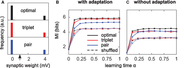
Figure 4. Triplets are better than pairs when the neuron adapts. (A) Distributions of synaptic efficacies obtained after learning. The weights were all initialized at 1 mV before learning (black arrow). When SFA is switched off, the very same bimodal distributions emerge (not shown). (B) Evolution of the MI along learning time. Learning time is arbitrarily indexed from 0 < α < 1. The dashed curves represent the MI when the weights taken from the momentary distribution at time α are shuffled. Each point is obtained from averaging the MI over 10 different shuffled versions of the synaptic weights. Error bars denote standard error of the mean (SEM) over 10 independent learning episodes with different input spike trains. (C) Same as in (B), but SFA is switched off. The y-scale is the same as in (B). Parameters for those simulations were λ = 0, γ = 0 with SFA, and γ = 1 without SFA. Other parameters took the values given in Table 1.

Triplet-based learning rule

We use the minimal model developed in Pfister and Gerstner (2006) with “all-to-all” spike interactions. Presynaptic spikes at synapse j leave a trace r_j (Figure 3B) which jumps by 1 after each spike and otherwise decays exponentially with time constant τ₊. Similarly, the postsynaptic spikes leave two traces, o₁ and o₂, which jump by 1 after each postsynaptic spike and decay exponentially with time constants τ₋ and τ_y respectively:

where x_j(t) and y(t) are sums of δ-functions at each firing time as introduced above. The synaptic weight w_j undergoes LTD proportionally to o₁ after each presynaptic spike, and LTP proportionally to r_jo₂ following each postsynaptic spike:

where η₃ denotes the learning rate. Note that o₂ is taken just before its update. Under the assumption that pre- and postsynaptic spike trains are independent Poisson processes with rates ρ_x and ρ_y respectively, the average weight change was shown in Pfister and Gerstner (2006) to be proportional to

The rule is thus structurally similar to a Bienenstock–Cooper–Munro (BCM) learning rule (Bienenstock et al., 1982) since it is linear in the presynaptic firing rates and non-linear in the postsynaptic rate. It is possible to roughly stabilize the postsynaptic firing rate at a target value ρ_targ, by having slide in an activity-dependent manner:

where is a starting value and is an average of the instantaneous firing rate on the timescale of seconds or minutes (time constant τ_ρ). Finally, is set to make ρ_targ an initial fixed point of the dynamics in Eq. 17:

The postsynaptic rate should therefore roughly remain equal to its starting value ρ_targ. In practice, the Poisson assumption is not valid because of adaptation and refractoriness, and independence becomes violated as learning operates. This causes the postsynaptic firing rate to deviate and stabilize slightly away from the target ρ_targ. We therefore always set ρ_targ empirically so that the firing rate stabilizes to the true desired target.

Pair-based learning rule

We use a pair-based STDP rule structurally similar to the triplet rule described by Eq. 16 (Figure 3B). The mechanism for LTD is identical, but LTP does not take into account previous postsynaptic firing:

where η₂ is the learning rate. also slides in an activity-dependent manner according to Eq. 18, to help stabilizing the output firing rate at a target ρ_targ. is set such that LTD initially balances LTP, i.e.,

Comparing learning rules in a fair way requires making sure that their learning rates are equivalent. Since the two rules share the same LTD mechanism, we can simply take the same value for as well as η₂ = η₃. Since LTD is dynamically regulated to balance LTP on average in both rules, this ensures that they also share the same LTP rate.

Weight bounds

In order to prevent the weights from becoming negative or from growing too large, we set hard bounds on the synaptic efficacies for all three learning rules, when not stated otherwise. That is, if the learning rule requires a weight change Δw_j, w_j is set to

This type of bounds, in which the weight change is independent of the initial synaptic weight itself, is known to yield bimodal distributions of synaptic efficacies. In the simulation of Figure 5, we also consider the following soft bounds to extend the validity of our results to unimodal distributions of weights:

where a is a free parameter and w₀ = 1 mV is the value at which synaptic weights are initialized at the beginning of all learning experiments. This choice of soft-bounds is further motivated in Section “Results.” The shapes of the LTP and LTD weight-dependent factors are drawn in Figure 5A, for a = 9. Note that the LTD and LTP factors cross at w₀, which ensures that the balance between LTP and LTD set by Eqs 19 and 21 is initially preserved.

FIGURE 5

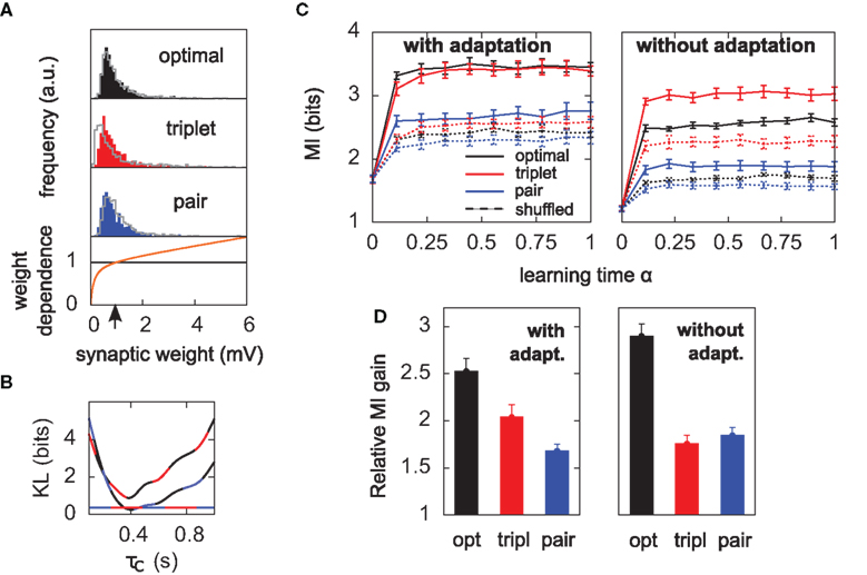
Figure 5. Results hold for “soft-bounded” STDP. The experiments of Figure 4 are repeated with soft-bounds on the synaptic weights (see Materials and Methods). (A) Bottom: LTP is weight-independent (black line), whereas the amount of LTD required by each learning rule (Δw < 0) is modulated by a growing function of the momentary weight value (orange curve). The LTP and LTD curves cross at w₀ = 1 mV, which is also the initial value of the weights in our simulations. Top: this form of weight dependence produces unimodal but skewed distributions of synaptic weights after learning, for all three learning rules. The learning paradigm is the same as in Figure 4. Gray lines denote the weight distributions when adaptation is switched off. Note that histograms are computed by binning all weight values from all learning experiments, but the distributions look similar on individual experiments. In these simulations λ = 0, a = 9, and τ_C = 0.4 s. (B) The parameter τ_C of the optimal learning rule has been chosen such that the weight distribution after learning stays as close as possible to that of the pair and triplet models. τ_C = 0.4 s minimizes the KL divergences between the distribution obtained from the optimal model and those from the pair (black-blue) and triplet (black-red) learning rules. The distance is then nearly as small as the triplet-pair distance (red-blue). (C) MI along learning time in this weight-dependent STDP scenario (cf. Figures 4B,C). (D) Normalized information gain (see text for definition).

When the soft-bounds are used, the parameter τ_C of the optimal model is adjusted so that the weight distribution obtained with the optimal rule best matches the weight distributions of the pair and triplet rules. This parameter indeed has an impact on the spread of the weight distribution: the optimal model knows about the generative model that underlies postsynaptic spike generation, and therefore takes optimally the noise into account, as long as τ_C spans no more than the width of the postsynaptic autocorrelation Toyoizumi et al. (2005). If τ_C is equal to this width (about 20 ms), some weights can grow very large (>50 mV), which results in non-realistic weight distributions. Increasing τ_C imposes more detrimental noise such that all weights are kept within reasonable bounds. In order to constrain τ_C in a non-arbitrary way, we ran the learning experiment for several values of τ_C and computed the KL divergences between weight distributions (optimal-triplet, optimal-pair). τ_C is chosen to minimize these, as shown in Figure 5B.

Simulation of in vitro Experiments

To obtain the predictions of the optimal model on standard in vitro STDP experiments, we compute the weight change of a single synapse (N = 1) according to Eq. 12. The effect of the remaining thousands of synapses is concentrated in a large background noise, obtained by adding a u_b = 19 mV baseline to the voltage. The gain becomes g_b = g(u_b) ≃ ( 21.45 Hz, which in combination with adaptation and refractoriness would yield a spontaneous firing rate of about 7.5 Hz (see Figure 1). Spontaneous firing is artificially blocked, however. Instead, the neuron is forced to fire at precise times as described below.

The standard pairing protocol is made of a series of pre–post spike pairs, the spikes within the same pair being separated by Δs = t_post − t_pre. Pairs are repeated with some frequency . The average is taken fixed and equal to g_b, considering that STDP is optimal for in vivo conditions such that should not adapt to the statistics of in vitro conditions. The homeostasis is turned off (γ = 0) in order to consider only the effects of the infomax principle.

Results

We study information transmission through a neuron modeled as a noisy communication channel. It receives input spike trains from a hundred plastic excitatory synapses, and stochastically generates output spikes according to an instantaneous firing rate modulated by presynaptic activities. Importantly, the firing rate is also modulated by the neuron’s own firing history, in a way that captures the SFA mechanism found in a large number of cortical cell types. We investigate the ability of three different learning rules to enhance information transmission in this framework. The first learning rule is the standard pair-based STDP model, whereby every single pre-before-post (resp. post-before-pre) spike pair yields LTP (resp. LTD) according to a standard double exponential asymmetric window (Bi and Poo, 1998; Song et al., 2000). The second one was developed in Pfister and Gerstner (2006) and is based on triplets of spikes. LTD is obtained similarly to the pair rule, whereas LTP is obtained from pairing a presynaptic spike with two postsynaptic spikes. The third learning rule (Toyoizumi et al., 2005) is derived from the infomax principle, under some metabolic constraints.

Triplet-STDP is Better than Pair-STDP When the Neuron Adapts

We assess and compare the performance of each learning rule on a simple spatio-temporal receptive field development task, with N = 100 presynaptic neurons converging onto a single postsynaptic cell (Figure 2A).

For each presynaptic neuron, a 5-s input spike train is generated once and for all (see Materials and Methods). All presynaptic spike trains are then replayed continuously 5,000 times. All synapses undergo STDP according to one of the three learning rules. Synaptic weights are all initially set to 1 mV, which yields an initial output firing rate of about 7.5 Hz. We set the target firing rate ρ_targ of each learning rule such that the output firing rate stays very close to 7.5 Hz. To gather enough statistics, the whole experiment is repeated 10 times independently, each time with different input patterns. All results are therefore reported as mean and standard error of the mean (SEM) over the 10 trials.

All three learning rules developed very similar bimodal distributions of synaptic efficacies (Figure 4A), irrespective of the presence or absence of SFA. This is a well known consequence of additive STDP with hard bounds imposed on the synaptic weights (Kempter et al., 1999; Song et al., 2000). The firing rate stabilizes at 7.5 Hz as desired, for all plasticity rules (not shown). In Figure 4B, we show the evolution of the MI (solid lines) as a function of learning time. It is computed as described in Section “Materials and Methods,” from the postsynaptic activity gathered during 100 periods (500 s). Since we are interested in quantifying the ability of different learning rules to enhance information transmission, we look at the information gain [defined as MI(α = 1) − MI(α = 0)] rather than the absolute value of the MI after learning. The triplet model reaches 98% of the “optimal” information gain while the pair model reaches 86% of it. Note that we call “optimal” what comes from the optimality model, but it is not necessarily the optimum in the space of solutions, because (i) a stochastic gradient ascent may not always lead to the global maximum, (ii) Toyoizumi et al.’s (2005) optimal learning rule involves a couple of approximations that may result in a sub-optimal algorithm, and (iii) their learning rule does not specifically optimize information transmission for our periodic input scenario, but rather in a more general setting where input spike trains are drawn continuously from a fixed distribution (stationarity).

It is instructive to compare how much information is lost for each learning rule when the synaptic weights are shuffled. Shuffling means that the distribution stays exactly the same, while the detailed assignment of each w_j is randomized. The dashed lines in Figure 4B depict the MI under these shuffling conditions. Each point is obtained from averaging the MI over 10 different shuffled versions of the weights. The optimal and triplet model lose respectively 33 and 32% of their information gains, while the pair model loses only 23%. This means that the optimal and triplet learning rules make a better choice in terms of the detailed assignment of each synaptic weight. For the pair learning rule, a larger part of the information gain is a mere side-effect of the weight distribution becoming bimodal. As an aside, we observe that the MI is the same (4.5 bits) in the “shuffled” condition for all three learning rules. This is an indication that we can trust our information comparisons. The result is also compatible with the value found by randomly setting 20 weights to the maximum value and the others to 0 (Figure 2B, square mark).

How is adaptation involved in this increased channel capacity? In Figure 2C, the MI is plotted as a function of the postsynaptic firing rate, for an adaptive (black dots) and a non-adaptive (gray dots) neuron, irrespective of synaptic plasticity. Each point in the figure is obtained by setting randomly a given fraction χ of synaptic weights to the upper bound (4 mV), and the rest to 0 mV. The weight distribution stays bimodal, which leaves the neuron in a high information transmission state. χ is varied in order to cover a wide range of firing rates. We see that adaptation enhances information transmission at low firing rates (<10 Hz). The MI has a maximum at 7.5 Hz when the neuron is adapting (black circles). If adaptation is removed, the peak broadens and shifts to about 15 Hz (green circles). If the energetic cost of firing spikes is also taken into account, the best performance is achieved at 3 Hz, whether adaptation is enabled or not. This is illustrated in Figure 2C (lower plot) where the information per spike is reported as a function of the firing rate.

Is adaptation beneficial in a general sense only, or does it differentially affect the three learning rules? To answer this question, we have the neuron learn again from the beginning, SFA being switched off. The temporal evolution of the MI for each learning rule is shown in Figure 4C. Overall, the MI is lower when the neuron does not adapt (compare Figure 4B and Figure 4C), which is in agreement with the previous paragraph and Figure 2C. Importantly, the triplet model loses its advantage over the pair model when adaptation is removed (compared red and blue lines in Figure 4C). This suggests a specific interaction between synaptic plasticity and the intrinsic postsynaptic dynamics in the optimal and triplet models. This is further investigated in later sections.

Finally, the main results of Figure 4 also hold when the distribution of weights remains unimodal. To achieve unimodal distributions with STDP, the hypothesis of hard-bounded synaptic efficacies must be relaxed. We implemented a form of weight-dependence of the weight change, such that LTP stays independent of the synaptic efficacy, while stronger synapses are depressed more strongly (see Materials and Methods). The weight-dependent factor for LTD had traditionally been modeled as being directly proportional to w_j (e.g., van Rossum et al., 2000), which provides a good fit to the data obtained from cultured hippocampal neurons by Bi and Poo (1998). Morrison et al. (2007) proposed an alternative fit of the same data with a different form of weight-dependence of LTP. Here we use a further alternative (see Materials and Methods, and Figure 5A). We require that the multiplicative factors for LTP and LTD exactly match at w_j = w₀ = 1 mV, where initial weights are set in our simulations. Further, we found it necessary that the slope of the LTD modulation around w₀ be less than 1. Indeed, our neuron model is very noisy, such that reproducible pre–post pairs that need to be reinforced actually occur among a sea of random pre–post and post–pre pairs. If LTD too rapidly overcomes LTP above w₀, there is no chance for the correlated pre–post spikes to evoke sustainable LTP. The slope must be small enough for correlations to be picked up. This motivates our choice of weight dependence for LTD as depicted in Figure 5A. The weight distributions for all three learning rules stay indeed unimodal, but highly positively skewed, such that the neuron can really “learn” by giving some relevant synapses large weights (tails of the distributions in Figure 5A). Note that the obtained weight distributions resemble those recorded by Sjöström et al. (2001) (see e.g., Figure 3C in their paper).

The evolution of the MI along learning time is reported in Figure 5C. Overall, MI values are lower than those of Figure 4B. Unimodal distributions of synaptic efficacies are less informative than purely bimodal distributions, reflecting the lower degree of specialization to input features. Such distributions may however be advantageous in a memory storage task where old memories which are not recalled often need to be erased to store new ones. In this scenario, strong weights which become irrelevant can quickly be sent back from the tail to the main weight pool around 1 mV. For a detailed study of the impact of the weight-dependence on memory retention, see Billings and van Rossum (2009).

We see that it is difficult to directly compare absolute values of the MI in Figure 5C, since the “shuffled” MIs (dashed lines) do not converge to the same value. This is because some weight distributions are more skewed than others (compare red and blue distributions in Figure 5A). In the present study, we are more interested in knowing how good plasticity rules are at selecting individual weights for up- or down-regulation, on the basis of the input structure. We would like our performance measure to be free of the actual weight distribution, which is mainly shaped by the weight- dependence of Eq. 23. We therefore compare the normalized information gain, i.e., [MI(α = 1) − MI(α = 0)] / [MI_sh(α = 1) − MI(α = 0)], where MI_sh denotes the MI for shuffled weights. The result is shown in Figure 5D: the triplet is again better than the pair model, provided the postsynaptic neuron adapts.

Our simulations show that when SFA modulates the postsynaptic firing rate, the triplet model yields a better gain in information transmission than pair-STDP does. When adaptation is removed, this advantage vanishes. There must be a specific interaction between triplet-STDP and adaptation that we now seek to unravel.

Triplet-STDP Increases the Response Entropy when the Neuron Adapts

Information transmission improves if the neuron learns to produce more diverse spike trains [H(Y^K) increases], and if the neuron becomes more reliable [H(Y^K|φ) decreases] In Figure 6A we perform a differential analysis of both entropies, on the same data as presented in Figure 4 (i.e., for hard-bounded STDP). Whether the postsynaptic neuron adapts (top) or not (bottom), the noise entropy (right) is drastically reduced, and the triplet learning rule does so better than the pair model (compare red and blue). The differential impact of adaptation on the two models can only be seen in the behavior of the response entropy H(Y^K) (left). When the postsynaptic neuron adapts, triplet- and optimal STDP both increase the response entropy, while it decreases with the pair model. This behavior is reflected in the interspike-interval (ISI) distributions, shown in Figure 6B. With adaptation, the optimal and triplet rules produce distributions that are close to an exponential (which would be a straight line in the logarithmic y-scale). In contrast, the ISI distribution obtained from pair-STDP stays almost flat for ISIs between 25 and 120 ms. Without adaptation, the optimal and triplet models further sparsifies the ISI distribution which then becomes sparser than an exponential, reducing the response entropy.

FIGURE 6

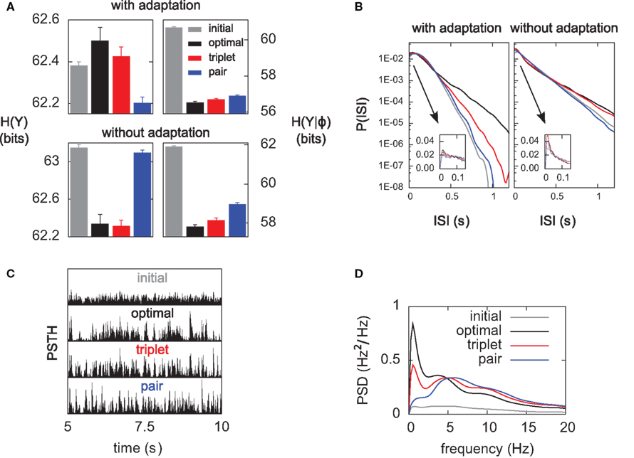
Figure 6. Differential analysis of the entropies. The learning experiments are the same as in Figure 4, using hard-bounds on the synaptic weights. (A) Response entropy (left) and noise entropy (right) with (top) and without (bottom) postsynaptic SFA. Entropies are calculated at the end of the learning process, except for the gray boxes which denote the entropies prior to learning. (B) Interspike-interval distributions with (left) and without (right) SFA, after learning (except gray line, before learning). The main plots have a logarithmic y-scale, whereas the insets have a linear one. (C) Peri-stimulus time histograms (PSTHs) prior to learning (top) and after learning for each learning rule, over a full 5-s period. All plots share the same y-scale. (D) Power spectra of the PSTHs shown in (C), averaged over the 10 independent learning experiments.

Qualitative similarities between the optimal and triplet models can also be found in the power spectrum of the peri-stimulus time histogram (PSTH). The PSTHs are plotted in Figure 6C over a full 5-s period, and their average power spectra are displayed in Figure 6D. The PSTH is almost flat prior to learning, reflecting the absence of feature selection in the input. Learning in all three learning rules creates sharp peaks in the PSTH, which illustrates the drop in noise entropy seen in Figure 6A (right). The pair learning rule produces PSTHs with almost no power at low frequencies (below 5 Hz). In contrast, these low frequencies are strongly boosted by the optimal and triplet models. This is however not specific to SFA being on or off (not shown). We give an intuitive account for this in Section “Discussion.”

This section has shed light on qualitative similarities in the way the optimal and triplet learning rules enhance information transmission in an adaptive neuron. We now seek to understand the reason why taking account of triplets of spikes would be close-to-optimal in the presence of postsynaptic SFA.

The Optimal Model Exhibits a Triplet Effect

How similar is the optimal model to the triplet learning rule? In essence, the optimal model is a stochastic gradient learning rule, which updates the synaptic weights at every time step depending on the recent input–output correlations and the current relevance of the postsynaptic state. In contrast to this, phenomenological models require changing the synaptic efficacy upon spike occurrence only. It is difficult to compress what happens between spikes in the optimal model down to a single weight change at spike times. However we know that the dependence of LTP on previous postsynaptic firing is a hallmark of the triplet rule, and is absent in the pair rule. We therefore investigate the behavior of the optimal learning rule on post–pre–post triplets of spikes, and find a clear triplet effect (Figure 7).

FIGURE 7

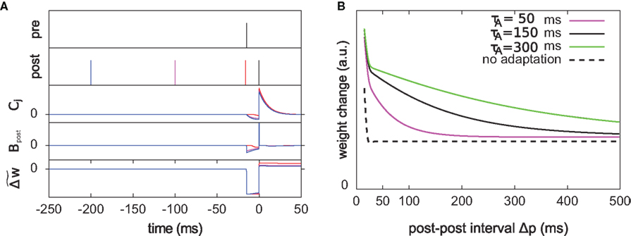
Figure 7. The optimal model incorporates a triplet effect when the postsynaptic neuron adapts. (A) A pre–post pair (Δs = 15 ms interval, black lines in the first two rows) is preceded by another postsynaptic spike. The post–post interval Δp is made either 16 (red line), 100 (purple), and 200 ms (blue). The time course of C_j, B_post, and the cumulative weight change are plotted in the bottom rows. (B) Total weight change (optimal model) as a function of the post–post interval, for various adaptation time constants, and without adaptation (dashed line).

We consider an isolated post–pre–post triplet of spikes, in this order (Figure 7A). Isolated means that the last pre- and postsynaptic spikes occurred a very long time before this triplet. Let , t_pre, and denote the spike times. The pre–post interval is kept constant equal to . We vary the length of the post–post interval from 16 to 500 ms. The resulting weight change is depicted in Figure 7B. For comparison, the triplet model would produce – by construction – a decaying exponential with time constant τ_y. In the optimal model, potentiation decreases as the post–post interval increases. Two times constants show up in this decay, which reflect that of refractoriness (2 ms) and adaptation (150 ms). The same curve is drawn for two other adaptation time constants (see red and blue curves). When adaptation is removed, the triplet effect vanishes (dashed curve). It should be noted that the isolated pre–post pair itself (i.e., large post–post interval) results in a baseline amount of LTP, which is not the case in the triplet model. Figure 7A shows how this effect arises mechanistically. Three different triplets are shown, with the pre–post pair being fixed, and the post–post interval being either 16, 100, or 200 ms (red, purple, and blue respectively).

To further highlight the similarity between the optimal learning rule and the triplet model, we now derive an analytical expression for the optimal weight change that follows a post–pre–post triplet of spikes. Let us observe that the final cumulated weight change evoked by the triplet is dominated by the jump that occurs just following the second postsynaptic spike (Figure 7A) – except for the negative jump of size λ that follows the presynaptic spike arrival, but this is a constant. Our analysis therefore concentrates on the values of and . Let us denote by the value of the unitary synaptic PSP at time . Around the baseline potential u_b = 19 mV, the gain function is approximately linear (cf. Figure 1A), i.e., where g_b = g(u_b) and are constants. From Eq. 14, we read which is approximately equal to

assuming the contribution of w_jε_j is small compared to the baseline gain g_b. The term proportional to M in Eq. 14 is negligible compared to the δ-function. From Eq. 13, we see that

The total weight change following the second postsynaptic spike is therefore

where

Since we have taken τ_C = τ_m, the first two exponentials collapse into ε_j. To carry out the integration, let us further simplify the adaptation model into , assuming that ms so that the refractoriness has already vanished at the time of the presynaptic spike, while adaptation remains. It is also assumed that the triplet is isolated, so that we can neglect the cumulative effect of adaptation. Eq. 27 becomes

If Δs ≪ τ_A, the last term into square brackets is approximately Δs/τ_A. If not, becomes so small that the whole r.h.s of Eq. 26 vanishes. To sum up, the total weight change following the second postsynaptic spike is given by

The first term on the r.h.s of Eq. 29 is a pair term, i.e., a weight change that depends only on the pre–post interval Δs. We note that it is proportional to , meaning that the time constant of the causal part of the STDP learning window is half the membrane time constant. The second term exactly matches the triplet model, when τ_A = τ_y and τ₊ = τ_m/2. Indeed, the triplet model would yield the following weight change:

From this we conclude that the triplet effect, which primarily arose from phenomenological minimal modeling of experimental data, also emerges from an optimal learning rule when the postsynaptic neuron adapts. To understand in more intuitive terms how the triplet mechanism relates to optimal information transmission, let us consider the case where the postsynaptic neuron is fully deterministic. If so, the noise entropy is null, so that maximizing information transfer means producing output spike trains with maximum entropy. If the mean firing rate ρ_targ is a further constraint, output spike trains should be Poisson processes, which as a by-product would produce exponentially distributed ISIs. If the neuron is endowed with refractory and adapting mechanisms, there is a natural tendency for short ISIs to appear rarely. Therefore, plasticity has to fight against adaptation and refractoriness to bind more and more stimulus features to short ISIs. The triplet effect is precisely what is needed to achieve this: if a presynaptic spike is found to be responsible for a short ISI, it should be reinforced more than if the ISI was longer. This issue is further developed in Section “Discussion.”

Optimal STDP is Target-Cell Specific

The results of the previous sections suggest that STDP may optimally interact with adaptation to enhance the channel capacity. In principle, if STDP is optimized for information transmission, it cannot ignore the intrinsic dynamics of the postsynaptic cell which influences the mapping between input and output spikes. The cortex is known to exhibit a rich diversity of cell types, with the corresponding range of intrinsic dynamics, and in parallel, STDP is target-cell specific (Tzounopoulos et al., 2004; Lu et al., 2007). Within the optimality framework, we should therefore be able to predict this target-cell specificity of STDP by investigating the predictions of the optimal model in the context of in vitro pairing experiments. Predictions should be made for different types of postsynaptic neurons, and be compared to experimental data. The optimal learning rule was shown in Toyoizumi et al. (2007) to share some features with STDP. We here extend this work to a couple of additional features including the frequency dependence. We also apply it to another type of postsynaptic cell, an inhibitory FS interneuron, for which in vitro data exist.

Only one synapse is investigated, with unit weight w₀ = 1 mV before the start of the experiment. Sixty pre–post pairs with given interspike time Δs are repeated in time with frequency f. The subsequent weight change given by Eq. 12 is reported as a function of both parameters (Figures 8A,B).

FIGURE 8

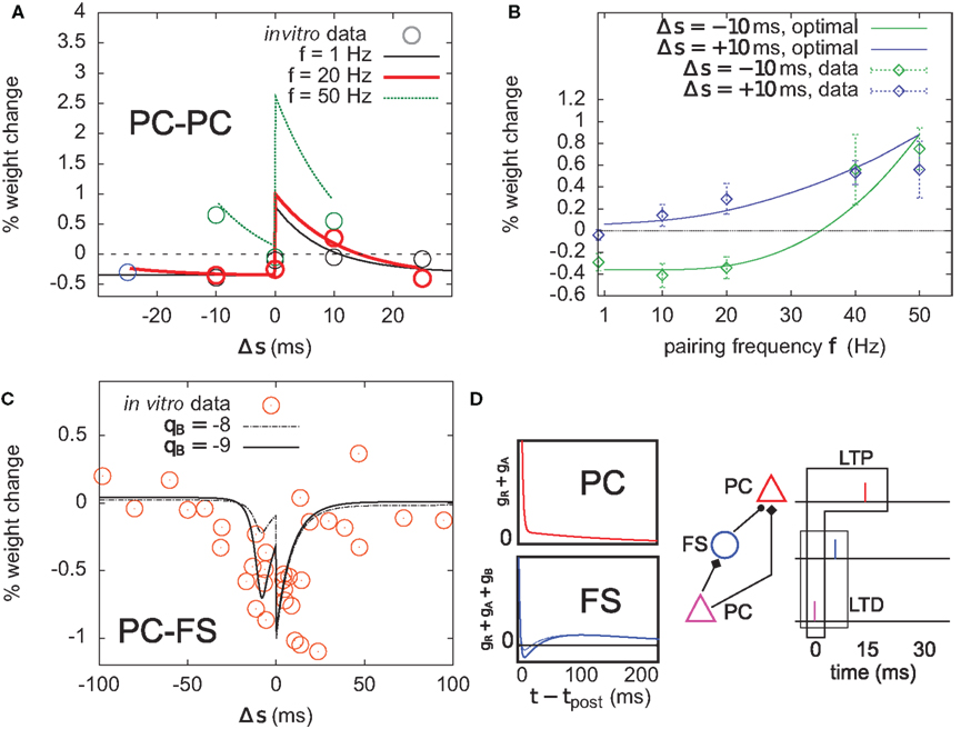
Figure 8. Optimal plasticity shares features with target-cell specific STDP. (A) The optimal model applied on 60 pre–post pairs repeating at 1 (black line), 20 (red thick), and 50 Hz (green) yields STDP learning windows that qualitatively match those recorded in Sjöström et al. (2001). For comparison, the in vitro data has been redrawn with permission. (B) LTP dominates when the pairing frequency is increased. The optimal frequency window is plotted for post-before-pre (−10 ms, solid green curve) and pre-before-post pairs (+10 ms, solid blue) repeated with frequency f (x-axis). Points and error bars are the experimental data, redrawn from Sjöström et al. (2001) with permission. (C) Learning window that minimizes information transmission at an excitatory synapse onto a fast-spiking (FS) inhibitory interneuron. The procedure is the same as in (A). The spike-triggered adaptation kernel was updated to better match that of a FS cell (see D). Dots are redrawn from Lu et al. (2007). (D) Left: after-spike kernels of firing rate suppression for the principal excitatory cell (red, same as the one we used throughout the article, see Materials and Methods) and the fast-spiking interneuron (blue). The latter was modeled by adding a third variable q_B < 0 with time constant τ_B = 30 ms to the initial kernel. Solid blue line: q_B = −9. Dashed blue line: q_B = −8. Right: schematic of a feed-forward inhibition microcircuit. A first principal cell (PC) makes an excitatory connection to another PC. It also inhibits it indirectly through a FS interneuron. The example spike trains illustrate the benefit of having LTD for pre-before-post pairing at the PC–FS synapse (see text).

The optimal model features asymmetric timing windows at 1, 20, and 50 Hz pairing frequencies (Figure 8A). At 1 and 20 Hz, pre-before-post yields LTP and post-before-pre leads to LTD. At 50 Hz the whole curve is shifted upwards, resulting in LTP on both sides. The model qualitatively agrees with the experimental data reported in Sjöström et al. (2001), redrawn for comparison (Figure 8A, circles).

The frequency dependence experimentally found in Markram et al. (1997) and Sjöström et al. (2001) is also qualitatively reproduced (Figure 8B). Post–pre pairing (Δs = −10 ms, green curve) switches from LTD at low frequency to LTP at higher frequencies, which is consistent with the timing windows in Figure 8A. For pre–post pairing (Δs = +10 ms, blue curve), LTP also increases with the pairing frequency. We also found that when SFA was removed, it was impossible to have a good fit for both the time window and the frequency dependence (not shown).

To further elucidate the link between optimal STDP and the after-spike kernel (g_R + g_A in Eq. 5), we ask whether plasticity at excitatory synapses onto FS interneurons can be accounted for in the same principled manner. In general, the intrinsic dynamics of inhibitory interneurons are very different from that of principal cells in cortex. STDP at synapses onto those cells is also different from STDP at excitatory-to-excitatory synapses (Tzounopoulos et al., 2004; Lu et al., 2007). The dynamics of FS cells are well modeled using a kernel which is shown in Figure 8D (Mensi et al., 2010). We augment the after-spike kernel with an additional variable g_B governed by

Parameters were set to τ_B = 30 ms, τ_A = 150 ms, q_B = −9, and q_A = 4. The resulting kernel (i.e., g_R + g_A + g_B – Figure 8D, blue kernel) exhibits after-spike refractoriness followed by a short facilitating period before adaptation takes over (note that the kernel is suppressive, meaning that positive values correspond to suppression of activity while negative values mean facilitation). Since interneurons do not project over long distances to other areas, the infomax objective function might not appear as well justified. Instead, let us consider the simple microcircuit shown in Figure 8D. A first principal cell (PC) makes an excitatory synapse onto a second PC, and we assume the infomax principle is at work. The first PC inhibits the second PC via a FS interneuron. How, intuitively, should the PC-to-FS synapse change so that the FS cell also contributes to the overall information maximization between the two PCs? In a very crude understanding of the infomax principle, if a pre-before-post pair of spikes is evoked at the PC–PC synapse (see spike trains in Figure 8D), the probability of having this pair again should be increased. If a similar pre-before-post pair is simultaneously evoked at the PC–FS synapse, then decreasing its weight will make it less likely that the FS spike again after the first PC. This in turn makes it more likely that the first PC–PC pair of spike will occur again. Therefore, PC–FS synapses should undergo some sort of anti-Hebbian learning. In fact, we found information minimization (i.e., the optimal model with opposite learning rate) to yield a good match between the simulated STDP time window (Figure 8C) and that found in Lu et al. (2007), which also exhibits LTD on both sides with some LTP at large intervals (see orange dots, superimposed). The post-before-pre part of the window can be understood intuitively: when a presynaptic spike arrives a few milliseconds after a postsynaptic spike, it falls in the period where postsynaptic firing is facilitated (q_B < 0). Therefore, it still has some influence on the subsequent postsynaptic activity. In order to avoid later causal pre–post events, the weight should be decreased. We see that the optimal STDP window depends on the after-spike kernel that describes the dynamical properties of the postsynaptic cell: q_B directly modulates the post–pre part of the window (see dashed curve in Figure 8C).

Together, these results suggest that if STDP is considered as arising from an optimality principle, it naturally interacts with the dynamics of the postsynaptic cell. This might underlie the target-cell specificity of STDP (Tzounopoulos et al., 2004; Lu et al., 2007).

Discussion

Experiments (Markram et al., 1997; Sjöström et al., 2001; Froemke et al., 2006) as well as phenomenological models of STDP (Senn et al., 2001; Froemke et al., 2006; Pfister and Gerstner, 2006; Clopath et al., 2010) point to the fact that LTP is not accurately described by independent contributions from neighboring postsynaptic spikes. In order to reproduce the results of recent STDP experiments, at least two postsynaptic spikes must interact in the LTP process. We have shown that this key feature (“triplet effect” in Pfister and Gerstner, 2006; Clopath et al., 2010; and similarly in Senn et al., 2001) happens to be optimal for an adapting neuron to learn to maximize information transmission. We have compared the performance of an optimal model (Toyoizumi et al., 2005) to that of two minimal STDP models. One of them incorporated the triplet effect (Pfister and Gerstner, 2006), while the second one did not (standard pair-based learning rule; Gerstner et al., 1996; Kempter et al., 1999; Song et al., 2000). The triplet-based model performs very close to the optimal one, and this advantage over pair-STDP disappears when SFA is removed from the intrinsic dynamics of the postsynaptic cell.

Our results are not restricted to additive STDP in which the amount of weight change is independent of the weight itself. It also holds when the amount of LTD increases with the efficacy of the synapse, a form which better reflects experimental observations (Bi and Poo, 1998; Sjöström et al., 2001). In the model introduced here, the amount of LTD is modulated by a sub-linear function of the synaptic weight. The deviation from linearity is set by a single parameter a > 0, with the purely multiplicative dependence of van Rossum et al. (2000) being recovered when a = 0. Since we modeled only a fraction of the total input synapses, we assumed a certain level of noise in the postsynaptic cell to account for the activity of the remaining synapses, thereby staying consistent with the framework of information theory in which communication channels are generally considered noisy. Because of this noise level, we found a large a was required for the weight distribution to become positively skewed as reported by Sjöström et al. (2001) (cortex layer V). For both the pair and triplet learning rules, the noisier the postsynaptic neuron, the weaker the LTD weight-dependence (i.e., the larger a) must be to keep a significant spread of the weight distribution. This means that other (possibly simpler) forms of weight dependence for LTD would work equally well, provided the noise level is adjusted accordingly. For example, in a nearly deterministic neuron, input–output correlations are strong enough for the weight-distribution to spread even when LTD depends linearly on the synaptic weight (a = 0, not shown).

In the original papers where the optimal and triplet rule were first described, it was pointed out that both rules could be mapped onto the BCM learning rule (Bienenstock et al., 1982). Both learning rules are quadratic in the postsynaptic activity. In turn, the link between the BCM rule and ICA has also already been researched (Intrator and Cooper, 1992; Blais et al., 1998; Clopath et al., 2010), as has the relationship between the infomax principle and ICA (Bell and Sejnowski, 1995). It therefore does not come as a surprise that the triplet model performs close to the infomax optimal learning rule. What is novel is the link to adaptation and spike after-potential.

We have also shown that when the optimal or triplet plasticity models are at work, the postsynaptic neuron learns to transmit information in a wider frequency band (Figure 6D): both rules evoke postsynaptic responses that have substantial power below 5 Hz, in contrast to the pair-based STDP rule. This is intuitively understood from the triplet effect combined with adaptation. Let us imagine STDP starts creating a peak in the PSTH so that we have, with high probability, a first postsynaptic spike at time t₀. If a presynaptic spike at time t₀ + (Δ/2) is followed by a further postsynaptic spike at time t₀ + Δ (Δ on the order of 10 ms), the triplet effect reinforces the connection from this presynaptic unit. In turn, it will create another peak at time t₀ + Δ, and this process can continue. Peaks thus extend and become broader, until adaptation becomes strong enough to prevent further immediate firing. The next series of peaks will then be delayed by a few hundred milliseconds. Broadening of peak widths and ISIs together introduce more power at lower frequencies in the PSTH.

One should bear in mind that neurons process incoming signals in order to convey them to other receivers. Although the information content of the output spike train really is an important quantity with respect to information processing, the way it can be decoded by downstream neurons should also be taken into account. Some “words” in the output spike train may be more suited for subsequent transmission than others. It has been suggested (Lisman, 1997) that since cortical synapses are intrinsically unreliable, isolated incoming spikes cannot be received properly, whereas bursts of action potentials evoke a reliable response in the receiving neuron. There is a lot of evidence for burst firing in many sensory systems (see Krahe and Gabbiani, 2004 for a review). As shown in Figure 6, the optimal and triplet STDP models tend to sparsify the distribution of ISIs, meaning that the neuron learns to respond vigorously (very short ISIs) to a larger number of features in the input stream, while remaining silent for longer portions of the stimulus. The neuron thus overcomes the effects of adaptation, which in baseline conditions (before learning) gives the ISI distribution a broad peak and a Gaussian-like drop-off. Our results therefore suggest that reliable occurrence of short ISIs can arise from STDP in adaptive neurons that are not intrinsic bursters. This is in line with Eyherabide et al. (2008), which recently provided evidence for high information transmission through burst activity in an insect auditory system (Locusta migratoria). The recorded neurons encoded almost half of the total transmitted information in bursts, and this was also shown not to require intrinsic burst dynamics.

Since our results rely on the outcome of a couple of numerical experiments, one might be concerned about the validity of the findings outside the range of parameter values we have used. There are for example a couple of free parameters in the neuron model. It is obviously difficult to browse the full high-dimensional parameter space and search for regions where the results would break down. We therefore tried to constrain our neuron parameters in a sensible manner. For example, the parameters of the SFA mechanism (q_A and τ_A) were chosen such that the response properties to a step in input firing rate would look plausible (Figure 1C). The noise parameter r₀ and the threshold value u_T were chosen so as to achieve an output rate of 7.5 Hz when all synaptic weights are at 1 mV. We acknowledge, though, that r₀ could be made arbitrarily large (reducing the amount of noise) since u_T can compensate for it. In the limit of very low noise, information transmission cannot be improved by increasing the neuron’s reliability anymore, since the noise entropy would already be minimal. We have shown however that a substantial part of the information gain found in the optimal and triplet models are due to an increased response entropy. This qualitative similarity, together with the structural similarities highlighted in Figures 7 and 8, lead us to believe that our results would still hold in the deterministic limit, and for noise levels in between. The optimal plasticity rule becoming ill-defined in this limit, we did not investigate this further.

To what extent can we extrapolate our results to the optimality of synaptic plasticity in the real brain? It obviously depends on the amount of trust one can put into this triplet model. Phenomenological models of STDP are usually constructed based on the results of in vitro experiments. They end up reproducing the quantitative outcome of only a few pre–post pairing schemes which are far from spanning the full complexity of real spike trains. To what extent can these models be trusted in more natural situations? From a machine learning perspective, a minimal model is likely to generalize better than a more detailed model, because its small number of free parameters might prevent it from overfitting the experimental data at the expense of its interpolation/extrapolation power. In this study, we have put the emphasis on an extrapolation of recent minimal models (Pfister and Gerstner, 2006; Clopath et al., 2010): the amount of LTP obtained from a pre-before-post pair increases with the recent postsynaptic firing frequency. By construction, the models account for the frequency dependence of the classical pairing experiment (they are fitted on this, among other things). However, they are seriously challenged by a more detailed study of spike interactions at L2/3 pyramidal cells (Froemke et al., 2006). There, it was explicitly shown that (n-posts)–pre–post bursts yield an amount of LTD which grows with n, the number of postsynaptic spikes in the burst preceding the pair. In contrast, post–pre–post triplets in hippocampal slices lead to LTP in a way that is consistent with the triplet model (Wang et al., 2005). The results of our study should therefore be interpreted bearing in mind the variability in experimental results. The recurrent in vitro versus in vivo debate should also be considered: synaptic plasticity depends on a lot of biochemical parameters for which the slice conditions do not faithfully reflect the normal operating mode of the brain.

A second controversy lies in our optimality model itself. While efficient coding of presynaptic spike trains may seem a reasonable goal to achieve at, say, thalamocortical synapses in sensory cortices, many other objectives could well be considered when it comes to other brain areas. Some examples are optimal decision making through risk balancing, reinforcement learning via reward maximization, or optimal memory storage and recall in autoassociative memories. It will be interesting to see more STDP learning rules in functionally different areas and how these relate to optimality principles.

Finally, while we investigated information transmission through a single postsynaptic cell, it remains to be elucidated how local information maximization in large recurrent networks of spiking neurons translates into a better information flow through the network.

Conflict of Interest Statement

The authors declare that the research was conducted in the absence of any commercial or financial relationships that could be construed as a potential conflict of interest.

Acknowledgments

This work was partially supported by the European Union Framework 7 ICT Project 215910 (BIOTACT, www.biotact.org). Jean-Pascal Pfister was supported by the Wellcome Trust. We thank Dr. Eilif Muller for having motivated the use of graphics cards (GPU) to compute the MI.

References

Bell, A. J., and Parra, L. C. (2005). “Maximising sensitivity in a spiking network,” in Advances in Neural Information Processing Systems, Vol. 17, eds L. K. Saul, Y. Weiss, and L. Bottou (Cambridge, MA: MIT Press), 121–128.

Bell, A. J., and Sejnowski, T. J. (1995). An information maximization approach to blind separation and blind deconvolution. Neural Comput. 7, 1129–1159.

Pubmed Abstract | Pubmed Full Text | CrossRef Full Text

Bell, C. C., V., H., Sugawara, Y., and Grant, K. (1997). Synaptic plasticity in a cerebellum-like structure depends on temporal order. Nature 387, 278–281.

Pubmed Abstract | Pubmed Full Text | CrossRef Full Text

Bi, G. Q., and Poo, M. M. (1998). Synaptic modifications in cultured hippocampal neurons: dependence on spike timing, synaptic strength, and postsynaptic cell type. J. Neurosci. 18, 10464–10472.

Pubmed Abstract | Pubmed Full Text

Bienenstock, E. L., Cooper, L. N., and Munro, P. W. (1982). Theory for the development of neuron selectivity: orientation specificity and binocular interaction in visual cortex. J. Neurosci. 2, 32–48.

Pubmed Abstract | Pubmed Full Text

Billings, G., and van Rossum, M. C. W. (2009). Memory retention and spike-timing dependent plasticity. J. Neurophysiol. 101, 2775–2788.

Pubmed Abstract | Pubmed Full Text | CrossRef Full Text

Blais, B. S., Intrator, N., Shouval, H., and Cooper, L. N. (1998). Receptive field formation in natural scene environments: comparison of single-cell learning rules. Neural Comput. 10, 1797–1813.

Pubmed Abstract | Pubmed Full Text | CrossRef Full Text

Bohte, S. M., and Mozer, M. C. (2007). Reducing the variability of neural responses: a computational theory of spike-timing-dependent plasticity. Neural Comput. 19, 371–403.

Pubmed Abstract | Pubmed Full Text | CrossRef Full Text

Chechik, G. (2003). Spike timing-dependent plasticity and relevant mutual information maximization. Neural Comput. 15, 1481–1510.

Pubmed Abstract | Pubmed Full Text | CrossRef Full Text

Clopath, C., Büsing, L., Vasilaki, E., and Gerstner, W. (2010). Connectivity reflects coding: a model of voltage-based STDP with homeostasis. Nat. Neurosci. 13, 344–352.

Pubmed Abstract | Pubmed Full Text | CrossRef Full Text

Clopath, C., Longtin, A., and Gerstner, W. (2008). “An online Hebbian learning rule that performs independent component analysis,” in Advances in Neural Information Processing Systems, Vol. 20, eds J. Platt, D. Koller, Y. Singer, and S. Roweis (Cambridge, MA: MIT Press), 321–328.

Eyherabide, H. G., Rokem, A., Herz, A. V. M., and I., S. (2008). Burst firing is a neural code in an insect auditory system. Front. Comput. Neurosci. 2, 1–17. doi: 10.3389/neuro.10.003.2008.

Pubmed Abstract | Pubmed Full Text | CrossRef Full Text

Florian, R. V. (2007). Reinforcement learning through modulation of spike timing-dependent synaptic plasticity. Neural Comput. 19, 1468–1502.

Pubmed Abstract | Pubmed Full Text | CrossRef Full Text

Froemke, R. C., Tsay, I., Raad, M., Long, J., and Dan, Y. (2006). Contribution of individual spikes in burst-induced long-term synaptic modification. J. Neurophysiol. 95, 1620–1629.

Pubmed Abstract | Pubmed Full Text | CrossRef Full Text

Gerstner, W., Kempter, R., van Hemmen, J., and Wagner, H. (1996). A neuronal learning rule for sub-millisecond temporal coding. Nature 383, 76–78.

Pubmed Abstract | Pubmed Full Text | CrossRef Full Text

Gerstner, W., and Kistler, W. K. (2002a). Mathematical formulations of Hebbian learning. Biol. Cybern. 87, 404–415.

CrossRef Full Text

Gerstner, W., and Kistler, W. (2002b). Spiking Neuron Models. New York: Cambridge University Press.

Intrator, N., and Cooper, L. (1992). Objective function formulation of the BCM theory of visual cortical plasticity – statistical connections, stability conditions. Neural Netw. 5, 3–17.

CrossRef Full Text

Izhikevich, E., and Edelman, G. M. (2008). Large-scale model of mammalian thalamocortical systems. Proc. Natl. Acad. Sci. U.S.A. 105, 3593–3598.

Pubmed Abstract | Pubmed Full Text | CrossRef Full Text

Kempter, R., Gerstner, W., and van Hemmen, J. L. (1999). Hebbian learning and spiking neurons. Phys. Rev. E 59, 4498–4514.

CrossRef Full Text

Klampfl, S., Legenstein, R., and Maass, W. (2009). Spiking neurons can learn to solve information bottleneck problems and to extract independent components. Neural Comput. 21, 911–959.

Pubmed Abstract | Pubmed Full Text | CrossRef Full Text

Krahe, R., and Gabbiani, F. (2004). Burst firing in sensory systems. Nat. Rev. Neurosci. 5, 13–23.

Pubmed Abstract | Pubmed Full Text | CrossRef Full Text

Lengyel, M., Kwag, J., Paulsen, O., and Dayan, P. (2005). Matching storage and recall: hippocampal spike timing-dependent plasticity and phase response curves. Nat. Neurosci. 8, 1677–1683.

Pubmed Abstract | Pubmed Full Text | CrossRef Full Text

Linsker, R. (1989). How to generate ordered maps by maximizing the mutual information between input and output signals. Neural Comput. 1, 402–411.

CrossRef Full Text

Lisman, J. (1997). Bursts as a unit of neural information: making unreliable synapses reliable. Trends Neurosci. 20, 38–43.

Pubmed Abstract | Pubmed Full Text | CrossRef Full Text

Lu, J., Li, C., Zhao, J.-P., Poo, M., and Zhang, X. (2007). Spike-timing-dependent plasticity of neocortical excitatory synapses on inhibitory interneurons depends on target cell type. J. Neurosci. 27, 9711–9720.

Pubmed Abstract | Pubmed Full Text | CrossRef Full Text

Magee, J. C., and Johnston, D. (1997). A synaptically controlled associative signal for Hebbian plasticity in hippocampal neurons. Science 275, 209–213.

Pubmed Abstract | Pubmed Full Text | CrossRef Full Text

Mensi, S., Naud, R., Avermann, M., Peterson, C., and Gerstner, W. (2010). Complexity and performance in simple neuron models. Front. Neurosci. doi: 10.3389/conf. fnins.2010.03.00064.

CrossRef Full Text

Markram, H., Lübke, J., Frotscher, M., and Sakmann, B. (1997). Regulation of synaptic efficacy by coincidence of postsynaptic AP and EPSPs. Science 275, 213–215.

Pubmed Abstract | Pubmed Full Text | CrossRef Full Text

Morrison, A., Aertsen, A., and Diesmann, M. (2007). Spike-timing dependent plasticity in balanced random networks. Neural Comput. 19, 1437–1467.

Pubmed Abstract | Pubmed Full Text | CrossRef Full Text

Morrison, A., Diesmann, M., and Gerstner, W. (2008). Phenomenological models of synaptic plasticity based on spike timing. Biol. Cybern. 98, 459–478.

Pubmed Abstract | Pubmed Full Text | CrossRef Full Text

Oja, E. (1982). A simplified neuron model as a principal component analyzer. J. Math. Biol. 15, 267–273.

Pubmed Abstract | Pubmed Full Text | CrossRef Full Text

Oja, E. (1989). Neural networks, principal components, and subspaces. Int. J. Neural Syst. 1, 61–68.

CrossRef Full Text

Olshausen, B. A., and Field, D. J. (1996). Emergence of simple-cell receptive field properties by learning a sparse code for natural images. Nature 381, 607–609.

Pubmed Abstract | Pubmed Full Text | CrossRef Full Text

Pfister, J.-P., and Gerstner, W. (2006). Triplets of spikes in a model of spike timing-dependent plasticity. J. Neurosci. 26, 9673–9682.

Pubmed Abstract | Pubmed Full Text | CrossRef Full Text

Pfister, J.-P., Toyoizumi, T., Barber, D., and Gerstner, W. (2006). Optimal spike-timing dependent plasticity for precise action potential firing in supervised learning. Neural Comput. 18, 1309–1339.

CrossRef Full Text

Rao, R. P., and Ballard, D. H. (1999). Predictive coding in the visual cortex: a functional interpretation of some extra-classical receptive-field effects. Nat. Neurosci. 2, 79–87.

Pubmed Abstract | Pubmed Full Text | CrossRef Full Text

Rubin, J., Lee, D. D., and Sompolinsky, H. (2001). Equilibrium properties of temporally asymmetric Hebbian plasticity. Phys. Rev. Lett. 86, 364–367.

Pubmed Abstract | Pubmed Full Text | CrossRef Full Text

Senn, W., Tsodyks, M., and Markram, H. (2001). An algorithm for modifying neurotransmitter release probability based on pre- and postsynaptic spike timing. Neural Comput. 13, 35–67.

Pubmed Abstract | Pubmed Full Text | CrossRef Full Text

Seung, H. S. (2003). Learning in spiking neural networks by reinforcement of stochastic synaptic transmission. Neuron 40, 1063–1073.

Pubmed Abstract | Pubmed Full Text | CrossRef Full Text

Sjöström, P., Turrigiano, G., and Nelson, S. (2001). Rate, timing, and cooperativity jointly determine cortical synaptic plasticity. Neuron 32, 1149–1164.

Pubmed Abstract | Pubmed Full Text | CrossRef Full Text

Smith, E. C., and Lewicki, M. S. (2006). Efficient auditory coding. Nature 439, 978–982.

Pubmed Abstract | Pubmed Full Text | CrossRef Full Text

Song, S., Miller, K. D., and Abbott, L. F. (2000). Competitive Hebbian learning through spike-time-dependent synaptic plasticity. Nat. Neurosci. 3, 919–926.

Pubmed Abstract | Pubmed Full Text | CrossRef Full Text

Sprekeler, H., Hennequin, G., and Gerstner, W. (2009). “Code-specific policy gradient rules for spiking neurons,” in Advances in Neural Information Processing Systems, Vol. 22, eds Y. Bengio, D. Schuurmans, J. Lafferty, C. K. I. Williams, and A. Culotta (Cambridge, MA: MIT Press), 1741–1749.

Sprekeler, H., Michaelis, C., and Wiskott, L. (2007). Slowness: an objective for spike-timing-dependent plasticity? PLoS Comput. Biol. 3, e112. doi: 10.1371/journal.pcbi.0030112.

Pubmed Abstract | Pubmed Full Text | CrossRef Full Text

Toyoizumi, T., Pfister, J.-P., Aihara, K., and Gerstner, W. (2005). Generalized Bienenstock–Cooper–Munro rule for spiking neurons that maximizes information transmission. Proc. Natl. Acad. Sci. U.S.A. 102, 5239–5244.

Pubmed Abstract | Pubmed Full Text | CrossRef Full Text

Toyoizumi, T., Pfister, J.-P., Aihara, K., and Gerstner, W. (2007). Optimality model of unsupervised spike-timing-dependent plasticity: synaptic memory and weight distribution. Neural Comput. 19, 639.

Pubmed Abstract | Pubmed Full Text | CrossRef Full Text

Tzounopoulos, T., Kim, Y., Oertel, D., and Trussell, L. (2004). Cell-specific, spike timing-dependent plasticity in the dorsal cochlear nucleus. Nat. Neurosci. 7, 719–725.

Pubmed Abstract | Pubmed Full Text | CrossRef Full Text

van Rossum, M. C. W., Bi, G. Q., and Turrigiano, G. G. (2000). Stable Hebbian learning from spike timing-dependent plasticity. J. Neurosci. 20, 8812–8821.

Pubmed Abstract | Pubmed Full Text

Wang, H.-X., Gerkin, R. C., Nauen, D. W., and Wang, G.-Q. (2005). Coactivation and timing-dependent integration of synaptic potentiation and depression. Nat. Neurosci. 8, 187–193.

Pubmed Abstract | Pubmed Full Text | CrossRef Full Text

Xie, X., and Seung, H. S. (2004). Learning in neural networks by reinforcement of irregular spiking. Phys. Rev. E 69, 041909.

CrossRef Full Text

Zhang, L. I., Tao, H. W., Holt, C. E., Harris, W. A., and Poo, M. M. (1998). A critical window for cooperation and competition among developing retinotectal synapses. Nature 395, 37–44.

Pubmed Abstract | Pubmed Full Text | CrossRef Full Text