Population coding of visual space: modeling

Introduction

Space serves as a framework for organizing our visual experience. An object is always perceived as having some extent and as existing at some location. The object itself will also generally have different parts in some sort of spatial relation to each other in a manner that defines object shape. Kant theorized that the spatial organization we experience of the world is imposed by the characteristics of our perceptual apparatus, which he argued produced a Euclidean visual space (Kant, 1781/1999). Helmholtz was among the first to empirically examine the spatial aspect of vision (Helmholtz, 1910/1962). His psychophysical investigations demonstrated that the geometry of visual space differed markedly from a Euclidean one. A vast body of psychophysical data since then corroborates Helmholtz, indicating that visual space is affected by both stimulus and task conditions in a manner difficult to describe by any fixed geometry (Wagner, 2006).

In this report we present a simple neural model for the representation of space. We explore how various known neural characteristics (such as increasing receptive field (RF) size with eccentricity) influence the spatial representation. In the model, location is represented by the collective activity of a population of neurons with different but overlapping tuning curves for space. These spatial tuning curves correspond to the RFs of visual neurons. The basic structure of this model, a population code constructed out of a set of overlapping tuning curves, is widely used for neural representations of various visual parameters (color, stereo depth, motion, etc.). As there were no synaptic interactions between neurons in the model (as is typical for models of population coding), the model did not form a neural network. We were primarily interested in the representation of space in visually responsive areas in occipital, parietal, inferotemporal, and prefrontal cortices, but some aspects of the approach developed here might transfer to other topics such as the construction of spatial maps for navigation in the hippocampus.

The model was restricted to consideration of 2D stimuli, as neural mechanisms for the extraction of depth information include additional mechanisms than those for the other two dimensions (although the final representation of space might not differ for the three dimensions). A frontoparallel plane (similar to a computer screen) defined the universe of all possible stimulus locations serving as inputs to the model. Given this stimulus set, the model did not include consideration of any depth cues, whether binocular (stereo, disparity, or vergence angle) or monocular (texture gradients, for example), and all stimulus representations were monocular. To a limited extent, neural representation of space in the depth domain has been considered previously (Lehky and Sejnowski, 1990). In addition, we were concerned solely with modeling retinotopic space and did not examine coordinate transforms to other frames of reference.

Algorithmically, the model revolved around statistical dimensionality reduction techniques. The number of dimensions for the spatial representation was reduced from the size of the neural population (up to several hundred thousand neurons) down to a 3D manifold embedded within the high-dimensional neural response space, dimensionally isomorphic with 3D physical space. We were particularly interested in how accurately such low-dimensional manifolds were able to capture the global geometry of standard Euclidean physical space. We shall argue that for some purposes the ability to form a low-dimensional representation of space may be computationally efficient (see also Sereno and Lehky, 2011).

A wide variety of dimensionality reduction methods are available (Lee and Verleysen, 2007; Izenman, 2008), both linear and non-linear. We focused on one of the oldest and most widely used non-linear techniques, multidimensional scaling (MDS). No claim is made that the brain is implementing these dimensionality reduction algorithms, and no attempt was made in the model to neurally implement any dimensionality reduction algorithm. We used MDS as a data analysis tool for data from a virtual monkey, where we could define and manipulate the precise characteristics of the neural population, mimicking different cortical areas’ known population characteristics. Using MDS tells us what information is available implicitly encoded within population activities. We suggest the brain is making use of that information. However, there are many ways to make use of the information and we do not wish to claim on the basis of available evidence that the brain is or is not implementing any particular algorithm.

In using population responses to reconstruct visual space, the model only had access to neural firing rates. That is, the response of each neuron was not labeled with additional information indicating RF properties for that neuron (RF peak location, RF diameter, and RF tuning curve shape). It is not clear in terms of biological mechanisms how all that additional information would be attached to the response of each neuron and communicated to the next neuron. If such information were available then the problem of spatial representation can become trivial, with just four spatially overlapping neurons sufficient to reconstruct 3D space through a process of trilateration. By not including information about tuning curve characteristics, our approach differs fundamentally from standard population decoding models based on Bayesian statistics or basis functions which do assume such information is available (Oram et al., 1998; Zhang et al., 1998; Deneve et al., 1999; Pouget et al., 2000; Averbeck et al., 2006; Jazayeri and Movshon, 2006; Quian Quiroga and Panzeri, 2009).

When recovering a parameter from neural population activity (in this case spatial position), the parameter must be specified relative to some coordinate system or frame of reference. For the Bayesian or basis function decoding models referenced above, the grid of tuning curves with labeled characteristics provides that reference frame. In that case the reference frame is said to be extrinsic as it is externally imposed on the stimulus by the RFs. For our model, tuning curve properties were not available and therefore could not serve as a reference frame. However, it is still possible to specify spatial position in terms of the relationships between objects that occupy the space (i.e., relative positions), which is what we did. Here the frame of reference is intrinsic. Extrinsic and intrinsic frames of reference are discussed by Lappin and Craft (2000). It is a general characteristic of MDS models, such as we use here, to specify recovered parameters within such an intrinsic reference frame. A consequence of using intrinsic reference frames is that information about scale, orientation, and position for a 2D spatial stimulus configuration is lost, although the relational structure of the configuration is retained. For the standard population coding models using extrinsic reference frames, the coding of sensory stimuli is atomistic as each stimulus point can be decoded without reference to any other stimulus point. On the other hand, for a decoding model based on an intrinsic reference frame, the coding is relational over a configuration of stimulus points (where we allow the configuration either to be physically present or built up within memory). Representation in terms of intrinsic reference frames therefore connect with Gestalt ideas about perception (Köhler, 1992). A recent model which shares our use of an intrinsic frame of reference to represent space is presented by Curto and Itskov (2008), which otherwise takes a different mathematical approach.

In recent years, MDS models of vision have focused on the representation of shape (Cutzu and Edelman, 1996; Edelman and Duvdevani-Bar, 1997; Sugihara et al., 1998; Edelman, 1999; Op de Beeck et al., 2001; Vogels et al., 2001; Kiani et al., 2007; Lehky and Sereno, 2007; Kriegeskorte et al., 2008). Ironically, little effort has gone into similar MDS studies on the representation of visual space, despite the inherently spatial nature of the technique (e.g., the standard textbook example of MDS involves the recovery of a spatial map of cities given a table of intercity distances). Previous applications of MDS in a spatial context include a neurophysiological study in monkey hippocampus (Hori et al., 2003), as well as several human psychophysical studies of space perception (Indow, 1968, 1982; Toye, 1986).

Although MDS can recover abstract shape spaces in those models oriented to shape perception, it is difficult to evaluate the accuracy of such recovered spaces as there is no objective standard to compare them to. That is, there is no universal metric to quantify shape similarity. On the other hand, we do know and can precisely quantify what physical space is like (it is Euclidian for scales that are behaviorally relevant), which gives us a standard with which to compare spatial representations recovered from population activity. Making such comparisons between physical space and recovered neural spatial representations will be the approach we use to evaluate the spatial representations. This does not mean that neurally-represented space ought to quantitatively match physical space, but that physical space can serve as a reference point for comparing neural space.

This modeling was motivated by actual spatial response data obtained from monkey neurophysiological recording in dorsal and ventral visually responsive cortex, described in the accompanying report (Sereno and Lehky, 2011). MDS methods, identical to those used in the model, were applied to that data in order to recover, compare, and better understand representations of visual space from those areas. This resulted in the observation that spatial representations differed substantially in the two cortical areas. The dorsal stream was able to represent space in a metrically accurate manner within a low-dimensional manifold while the ventral stream was not able to do so (recovering only a topologically- or categorically-correct spatial representation). One goal of the modeling here, therefore, was to understand how differences in such recovered spatial representations might arise from differences in the RF characteristics of neural populations in different cortical areas.

Materials and Methods

Receptive Field Size and Shape

Receptive field centers were spread in two dimensions, forming a regular hexagonal array (Figure 1) in most simulations. The RF for each neuron was a 2D Gaussian curve. Peak heights for all neurons were normalized to 1.0 unless otherwise noted. Neurophysiological data in both the ventral visual stream (AIT, Op de Beeck and Vogels, 2000) and dorsal visual stream (LIP, Ben Hamed et al., 2001) indicate that RFs in higher extrastriate areas have spatial tuning curves that are approximately Gaussian. The response r for such a RF was given by:

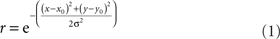
Receptive field diameter was specified by the space constant σ. Examples of populations with different RF diameters are shown in Figure 1A. Tails of the Gaussian tunings curves were not truncated and therefore extended across the whole visual field. As a consequence of that, each stimulus point stimulated the entire population of tuning curves.

FIGURE 1

Figure 1. Illustration of parameters describing the neural population for encoding space. Green dots mark the locations of receptive field centers. Black circles indicate receptive field diameter, with radius equal to one space constant σ of the 2D Gaussian spatial tuning curve. In the model, characteristics of the encoding population are defined by (A) Receptive field diameter, (B) Spacing between receptive field centers, (C) Dispersion of receptive field centers.

We also examined the effect of changing RF shape in two ways. The first variant was elliptical RFs. These were described by:

The anisotropy was produced by setting the x and y space constants to be unequal, σ_y = 3σ_x, producing the elongated fields with the major axis aligned vertically (Figure 18A). The other RF variant included surround inhibition. That was done using RFs described by Difference of Gaussians (DOG):

after which peak height was normalized to 1.0. This equation produced a RF shape in which the excitatory region was approximately the same size and shape as produced by Eq. 1, but with inhibitory regions added at the periphery (Figure 16A).

Receptive Field Spacing

Another parameter defining the encoding population was RF spacing- the distance separating two RF centers. This is illustrated in Figure 1B. Although primarily working with constant RF spacing on a regular hexagonal grid, we also examined the consequences of having randomly distributed RF centers (Figures 20A,B). In particular, Gaussian distributed RF centers resulted in more model neurons devoted to foveal and parafoveal representations, more closely mimicking cortical representations.

Receptive Field Dispersion

A third population parameter we varied was the dispersion of RF centers (Figure 1C). The RF center dispersion was the visual field range (diameter) over which RF centers extended. If the RF centers were narrowly dispersed they would be confined to within a region close to the foveal representation (for example, all RF centers confined within a circle 4° in diameter). Representations with narrow RF dispersion are foveally emphasized. A wide dispersion would have RF centers spread over a broader area. RF center dispersion was defined purely in terms of RF center locations. It did not include the outer edges of the RF regions around the periphery. High-level structures in both the ventral visual stream (AIT, Op de Beeck and Vogels, 2000) and dorsal visual stream (LIP, Ben Hamed et al., 2001) have relatively narrow RF dispersions compared to striate cortex.

Number of Model Neurons

The number of model neurons in the population was set by the requirement to fill a hexagonal grid. The number of locations in the grid was determined by the RF spacing between units and RF dispersion. Smaller RF spacing or greater RF dispersion led to a larger number of neurons. Hence, changing the RF spacing parameter (see Receptive Field Spacing, above), by definition, changed the number of RFs stimulated by a single point.

Stimulus Input in Physical Space

As an input to the model we generally used a grid of stimulus points in physical space arranged along a polar coordinate grid, such as shown in Figure 2. Those points were presented as stimuli to the neural population one at a time, producing a different neural response vector for each of the locations. By using a discrete grid of stimulus locations as input rather than a continuous pattern, we follow the same approach used in experimental investigations of spatial perception established by Helmholtz in the mid-nineteenth century (Helmholtz, 1910/1962) and used to the present day in both human and monkey studies (see, e.g., companion report, Sereno and Lehky, 2011).

FIGURE 2

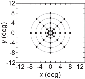
Figure 2. Typical configuration of points in physical space that served as input to the model. It consisted of 40 points arranged in a polar grid. The center of the grid corresponded to visual fixation. The points were arranged over five eccentricities, at [1, 2, 4, 6, 8] degrees of visual angle. At each eccentricity, eight points were placed in a circle at 45° increments.

Multidimensional Scaling

Multidimensional scaling was carried out using the Matlab Statistics Toolbox. Neural response vectors from the stimulus configuration were then fed into a classical MDS analysis (Young and Householder, 1938; Shephard, 1980; Borg and Groenen, 1997). The output of MDS was a set of geometrical coordinates, one for each stimulus location, corresponding to the relative spatial positions of stimulus points as encoded within the neural population. As detailed below, a measure of distortion was then calculated comparing the original spatial configuration in physical space with the spatial configuration that was recovered from the model’s neural encoding of space. The effect of model parameters (RF diameter, etc.) on the level of spatial distortion within the neural encoding could then be examined. In addition to the eight points at each eccentricity depicted in Figure 2, we added a ninth point at an angle of 22.5° to introduce an asymmetry in the grid, which aided in aligning the neural and physical coordinate systems when using the Procrustes transform as described below, but we did not use this extra point for error calculations. We were not generally concerned with the selectivity of the model neurons to stimulus shape, assuming that this population of neurons was responsive to the stimulus that was presented (although shape effects are considered in Figure 10).

Multidimensional scaling is a non-linear algorithm that takes as input a matrix of distances between all the response vectors and produces as output a spatial configuration of points that reproduces those distances. It proceeds iteratively to minimize an error function between the original distances and distances in the output spatial configuration.

Given n neurons in the population, presenting a stimulus at a particular location led to a pattern of activation described by a vector with n components. Each component of the vector indicated the firing rate, under that stimulus condition, for one neuron. For a stimulus at location a, we obtained the vector a₁, a₂, a₃,…a_n, and for a stimulus at location b, the vector b₁, b₂, b₃,…b_n, having a different pattern of activation.

As a first step in the implementation of the spatial MDS analysis, a measure of the distances between different response vectors must be computed. It is possible to define a variety of distance measures, but the one we used was based on the correlation between vectors. The distance d between two response vectors was defined as d = 1 − r, where r was the Pearson correlation coefficient between vectors, calculated on a component-by-component basis. Under a correlation-based measure, the distance between two response vectors depends on the angle between the vectors and not the lengths of the vectors. The correlation coefficient is equal to the cosine of the angle between response vectors (if they are centered to mean zero), giving a more geometric interpretation of r.

A correlation-based measure has the advantage over a Euclidean one in not being sensitive to overall changes of the level of activity in the population, but rather emphasizing changes in the pattern of population activity. For example, if moving from one stimulus condition to another caused or coincided with a doubling of the activity of all neurons, that would lead to a doubling of the Euclidean distance between the two response vectors, but zero distance under a correlation-based measure because the relative activities of the different neurons had not changed. This could occur in a biological system due to changes in animal alertness, for example.

For n neurons in the encoding population, the population response to a stimulus at a particular location can be represented by a point in n-dimensional space. With data from k locations, we have k points in n-dimensional space. In the model, populations were large, ranging from hundreds of neurons to hundreds of thousands of neurons, depending on the parameters chosen. Thus information about spatial location was embedded within a very high-dimensional space. The purpose of MDS was to reduce the dimensionality of the spatial representation (Lee and Verleysen, 2007), allowing examination of how accurately space could be represented within low-dimensional manifolds under different RF characteristics for the encoding population.

If we have data for stimuli at k locations, then there are k response vectors. Calculating the distances between all possible pairs of response vectors leads to a k × k matrix containing those values, called the distance matrix. The distance matrix served as the immediate input to the MDS analysis. The MDS algorithm includes, by definition, the constraint that those distances be preserved as much as possible when calculating a low-dimensional approximation to the data. By preserving inter-point distances at low dimensions, the relative spatial configuration amongst the points was preserved, giving us a map of global space as represented within a low-dimensional manifold by the neural population.

It should be noted that whether or not population responses lie on a low-dimensional manifold reflects inherent geometrical properties of those responses, independent of MDS or any other dimensionality reduction method. MDS does not cause responses to lie on a low-dimensional manifold, but merely serves as an analytic tool that reports whether such a low-dimensional manifold exists.

“Low-dimensional” in practice meant we projected high-dimensional population activity down to a 3D neural response manifold, as physical space is 3D. The physical stimulus was 2D, so that the recovered spatial representation ought to have been confined to a 2D subspace within that 3D manifold, if the geometry of neural space were dimensionally isomorphic to the geometry of physical space. Spatial distortion in the 2D representation of a 2D stimulus would be mathematically indicated by extension of the representation into higher dimensions in the MDS analysis.

We interpreted the third dimension derived from the MDS analysis as representing a third physical dimension (depth), analogous to the way the first two MDS dimensions were interpreted as representing the other two physical dimensions. This meant that curvature into the third MDS dimension was interpreted as distortion in which the flat physical stimulus has now become curved in depth within its neural representation. This interpretation was attractive as there is extensive psychophysical evidence that flat, frontoparallel patterns are indeed perceived as curving in space, originating with Helmholtz’s work (Helmholtz, 1910/1962) and moving forward into more modern times (Ogle, 1962; Foley, 1966; Wagner, 2006). Distortions into mathematical dimensions greater than three would simply be indicative of misplaced locations within a 3D space. Typically such higher-dimensional distortions were small in magnitude.

We found that some neural population parameters produced spatial representations that were dimensionally isomorphic to physical space, while others did not produce such isomorphism. Whether actual neural representations of space are isomorphic of course remains an empirical question, explored in the accompanying paper (Sereno and Lehky, 2011).

Procrustes Transform

The Procrustes transform was used to help quantify the amount of distortion between the physical configuration of stimulus points and the configuration of points recovered by MDS. This transformation was only used as a tool to evaluate MDS results, and no claim is made that it occurs in vivo.

The output from MDS was a set of k geometrical coordinates defining the relative locations of stimulus points as extracted from neural activities. Because the coordinates were extracted from distances between population vectors whose elements are firing rates, the scale was arbitrary and did not correspond to any physical unit such as centimeters or degrees of visual angle. Also, as MDS only extracts relative positions, the coordinate system of the recovered points could be rotated and reflected relative to physical space. Such an arbitrary linear transform in the neural representation of space is not a problem, just as the upside-down optical projection of the world on the retina is not a problem.

To quantitatively compare the recovered neural space with the original physical space, both must be transformed to the same coordinate system. To accomplish that, we used the Procrustes transform, a formalism that allowed us to quantify how accurately relative positions were recovered. The Procrustes transform linearly scaled, rotated, and reflected the geometrical coordinates output by MDS in such a manner as to minimize an error measure between stimulus coordinates in neural space and the stimulus coordinates in physical space. The error measure we used, called stress, was the square root of the normalized sum of squared errors between the two sets of coordinates:

In the equation, d_ij is the physical Euclidean distance between stimulus locations i and j, is the distance recovered by MDS from the neural population representation, and 〈•〉 is the mean value operator. The denominator normalizes the error by the scale of the distances. The Procrustes calculations were done in three dimensions. As the physical stimulus points were 2D, we set the value of the third physical dimension equal to zero for all points when doing the calculations.

If the representation of space within a 3D neural manifold was simply a linear transform of physical space, then stress would be zero. If there was a residual non-zero stress after performing the Procrustes transform, then there would be a non-linear distortion between physical space and the neural representation (the relative positions of stimulus points would be incorrectly represented). Greater stress indicates greater spatial distortion implicit within the neural population coding. Thus, by calculating stress we have a measure of the accuracy of the low-dimensional neural encoding of space. When plotting spatial positions recovered by the model, we show outputs of the Procrustes transform unless otherwise noted.

Besides looking at stress values, a second independent way to quantify the performance of the analysis is to examine the eigenvalues associated with the MDS output. Eigenvalues were calculated from the matrix Y × Y′ where Y was the MDS output matrix of recovered spatial positions, each matrix row representing a single position. If there are n neurons in the encoding population, the original representation of visual space has n dimensions. After the MDS analysis there are still n dimensions, but the n-dimensional space has been transformed so that most of the variance can be explained by a small number of those dimensions. Associated with each dimension in the MDS output is an eigenvalue that indicates how much of the variance is accounted for by that dimension. If MDS has been successful in reducing the dimensionality of the population representation, then only a few of these eigenvalues will be large and most will be close to zero. When all the eigenvalues are normalized such that their sum is 1.0, then the values of the normalized eigenvalues indicate the fraction of variance in the data that is accounted for by each dimension. We then pick those dimensions whose eigenvalues account for a large fraction of the total and use them to form a low-dimensional approximation of the original data. Ideally, for our conditions with stimuli confined to two dimensions within 3D physical space, to produce an isomorphic representation, the reconstructed neural space should have only two dimensions with non-zero eigenvalues, both of them equal to 0.5, and the rest of the dimensions should have zero eigenvalues.

Results

Spatial representations formed by the encoding population of neurons were examined as a function of the characteristics of the RFs forming the population.

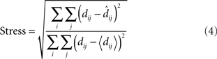
The effect of changing RF diameter is shown in Figure 3. As the analysis was done in three dimensions corresponding to physical space, the spatial coordinates of the stimulus points recovered from the population activity were also in three dimensions, even though the original physical stimulus was flat on the frontoparallel plane. The left column of Figure 3 plots these recovered points projected onto two dimensions (frontal plane), to facilitate comparison to the 2D physical configuration. The right column plots the side view, showing the curvature of the recovered representation into the third dimension (depth). Because MDS results are equivocal concerning the sign of the recovered coordinates, whether the curvature along the z coordinate is toward or away from the observer cannot be determined; here and in all following plots we follow the convention that curvature is away from the observer.

FIGURE 3

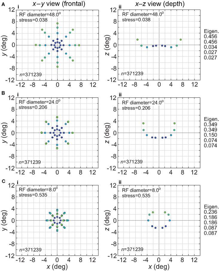
Figure 3. Spatial representation recovered by the model, for different receptive field diameters. (A) RF diameter = 48° (B) RF diameter = 24° (C) RF diameter = 8°. The number of model neurons in the encoding population is indicated by n. For each receptive field diameter, the left column shows the spatial representation in the x-y or frontoparallel plane. The right column shows curvature of the recovered spatial representation in the z-axis direction, caused by spatial distortion introduced by the neural coding. The x-z plots in the right column are taken along a cross-section of space corresponding to the y = 0 axis. Normalized eigenvalues associated with the multidimensional scaling procedure are displayed to the right of each row. RF dispersion was 64°, RF spacing was 0.1°, and the stimulus configuration was a 16° diameter grid as in Figure 2. Dots are color coded by eccentricity of physical stimulus, in order to ease interpretation of recovered spatial configurations that are highly distorted.

As the physical stimulus had no variation in depth, this curvature in depth is an indication of distortion in a low-dimensional neural representation of space. The eigenvalues in Figure 3 give another indication of spatial distortion. Ideally only two dimensions should have non-zero eigenvalues to represent the 2D stimulus configuration in a dimensionally isomorphic manner, but here we see non-zero eigenvalues spreading into higher dimensions.

For very large RFs (Figure 3A), the spatial representation recovered from the population activity has a high degree of accuracy in a 3D manifold. This is shown by the low value of stress between the configuration of the physical stimulus and the recovered configuration (stress = 0.038). As RF diameter becomes smaller, spatial distortion increases. The higher distortion is indicated by the increase in stress (stress = 0.535, Figure 3C) and also by the increase in eigenvalues beyond the first two dimensions as one goes down the rightmost column in Figure 3.

Increased distortion as RF diameters shrink is also apparent directly from inspection of the plots in Figure 3. The spatial representation is most accurate near fixation, and becomes increasingly distorted toward the periphery. The distortion has the effect of contracting the representation of peripheral points in the stimulus configuration inward toward the center. This 2D contraction is accompanied by increased curvature into the third dimension. If RF size is sufficiently small, distortion at large eccentricities becomes so great that the 2D representation of the most peripheral ring of points crosses inside more central rings (Figure 3C). The 2D topological ordering of points from the original physical stimulus configuration has been lost.

The effect of varying another population parameter, the dispersion of RF centers, is examined in Figure 4. A RF centers dispersion of 64° means that all RF centers are confined within a circle of diameter 64° centered on the foveal representation, or, equivalently, that all RF centers are within 32° of the foveal representation. As will be discussed later, the dispersion of RF centers is known to vary greatly between different cortical visual areas, so this parameter sheds light on the spatial consequence of that variation. We found that the accuracy of spatial representations within a low-dimensional manifold does depend strongly on the dispersion of RF centers, with accuracy decreasing when the RF centers are narrowly confined to a central region for large RF sizes.

FIGURE 4

Figure 4. Spatial representation recovered by the model, for different receptive field dispersions. (A) RF dispersion = 64° diameter (B) RF dispersion = 24° diameter (C) RF dispersion = 8° diameter. For each dispersion value, left column shows the spatial representation in the x-y or frontoparallel plane. The right column shows curvature of the recovered spatial representation in the z-axis direction, caused by spatial distortion introduced by the neural coding. RF diameter was 48°, RF spacing was 0.1°, and the stimulus configuration was a 16° diameter grid.

Comparing Figures 3 and 4, the spatial distortion caused by narrow RF center dispersion differs in nature from that caused by small RF diameter. For narrowly dispersed RF centers, although the representation becomes highly distorted, topological ordering is never lost. On the other hand, for small RF diameter the topological ordering is lost.

Spatial distortion, as measured by stress, is shown as a function of both RF diameter and RF dispersion in Figure 5. Stress plots are shown for three spatial configurations of the stimulus input, differing in diameter. The middle row in Figure 5 corresponds to the stimulus configuration used in Figures 3 and 4. In MDS studies, a stress level of 0.1 is conventionally assigned as the boundary between a “good” representation and a “poor” representation (Borg and Groenen, 1997), though like the p = 0.05 criterion for statistical significance, this is entirely arbitrary. A biological criterion of what constitutes a good representation could eventually be based on psychophysical discrimination studies.

FIGURE 5

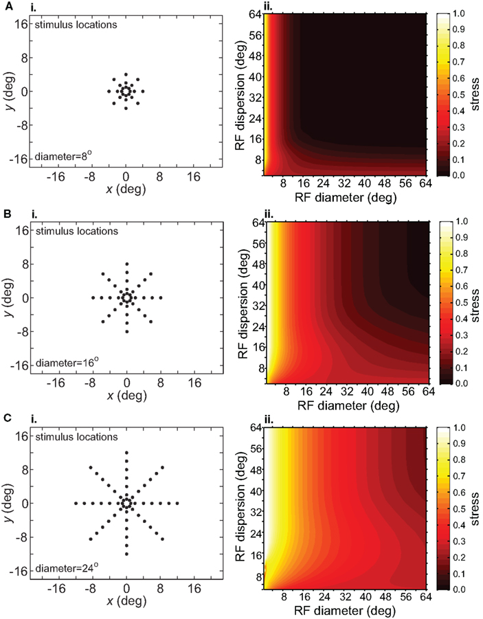
Figure 5. Three-dimensional plot of stress as a function of RF diameter and RF dispersion, using grid stimulus configurations. (A) 8° diameter stimulus grid. (B) 16° diameter stimulus grid. (C) 24° diameter stimulus grid.

Figure 5 confirms that RF diameter and RF dispersion are both important parameters affecting the accuracy of the spatial representation. When using grid stimulus patterns, the lowest distortions occur when both those parameters have large values. The decreased accuracy when RF center dispersion is narrow occurs even when the RFs are very large. Likewise, there is decreased accuracy when RF diameter is small, even when there is large dispersion. With large RFs, multiple overlapping RFs cover the peripheral visual field, but that is not sufficient to form an accurate large-scale spatial map. The RF centers must also spread out over the periphery.

We can create the converse of a narrowly focused RF center dispersion by arranging a “foveal-sparing” distribution of RF centers to form an annulus around the foveal region (e.g., Motter and Mountcastle, 1981). In our simulations, removing the foveal representation did not reduce the accuracy of spatial representations, and even improved them very slightly.

To verify that the observed sensitivity to RF diameter and dispersion did not reflect an idiosyncrasy of the MDS technique, we tried the same analysis procedure using a different dimensionality reduction algorithm, principal components analysis (PCA). The resulting stress plot for PCA is shown in Figure 6, corresponding to the stimulus configuration used in Figure 5B for the MDS analysis. The contours for the PCA stress plot qualitatively resemble those of the MDS stress plot (lowest stress values when both RF diameter and RF dispersion are large), except that in the PCA plot the entire surface is shifted to higher stress values. Those higher stress values may reflect limitations in the PCA algorithm, a linear dimensionality reduction method, compared to MDS, a non-linear method, in extracting optimal low-dimensional approximations to the original high-dimensional neural response data.

FIGURE 6

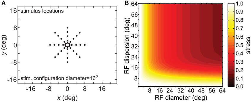
Figure 6. Three-dimensional plot of stress using principal components analysis rather than multidimensional scaling. (A) Spatial configuration of stimulus, which was a 16° diameter stimulus grid as used in Figure 5B. (B) Stress plotted as a function of RF diameter and RF dispersion.

Although RF diameter and RF dispersion were found to be important parameters, RF spacing did not have a major effect on spatial representations. Figure 7 shows that a plot of stress as a function of RF spacing is flat going out to inter-neuron spacings of several degrees. Visual cortical RF spacing in actuality is some small fraction of a degree, well within the flat portion of the graph. For a biologically plausible range, therefore, the accuracies of spatial representations are not sensitive to the RF spacing of the encoding population. In addition, changing RF spacing also changes the effective number of RFs stimulated by a single point (see Figure 1B). Thus, as shown in Figure 7, the number of neurons in the model had a negligible effect on the results.

FIGURE 7

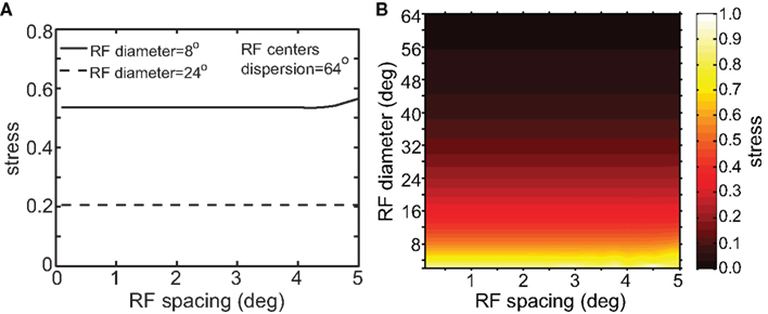
Figure 7. Stress as a function of RF spacing. (A) 2D plot, at selected values for RF diameter and RF dispersion. (B) 3D plot of stress as a function of RF diameter and RF spacing. These plots show that RF spacing has a negligible effect on stress.

A significant result shown in Figure 5 is that the accuracy of the spatial representation decreased for larger stimulus configurations. Interestingly, the stress plots for different-sized stimulus configurations are close to scaled copies of each other. Taking a square from the lower left corner of the stress plot for a small stimulus configuration and expanding it produces the approximate plot for a large stimulus.

The size-effect plots in Figure 5 confound two variables: the diameter of the stimulus configuration and the number of points in the configuration. To separate those factors we conducted two other sets of simulations. First, we kept the number of points constant while changing diameter by using ring-shaped stimulus configurations rather than grids. Second, we changed the number of points in a ring without changing its diameter.

Increasing the diameter of the stimulus ring increased distortion of the recovered spatial configuration (Figure 8), showing that stimulus spatial scale does matter. On the other hand, increasing the number of points in a ring did not change distortion to a large extent (compare Figure 9 with Figure 8B). Notably, all ring configurations had much lower stress than grid configurations, indicating difficulty in dealing with multiple eccentricities simultaneously. Overall, it appears more difficult to form an accurate global representation as the region of space included in the representation increases.

FIGURE 8

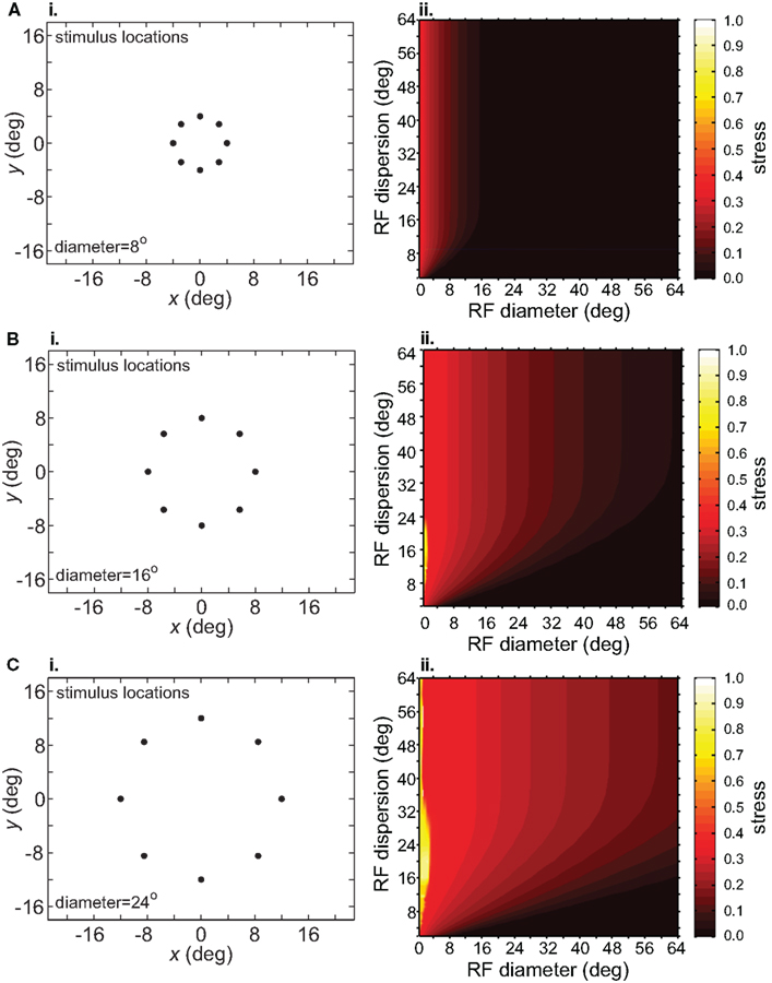
Figure 8. Effect of stimulus scale on recovered spatial representations. 3D plots of stress as a function of RF diameter and RF dispersion, using ring stimulus configurations with different diameters. (A) 8° diameter stimulus ring. (B) 16° diameter stimulus ring. (C) 24° diameter stimulus ring.

FIGURE 9

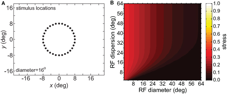
Figure 9. Effect on recovered spatial representations of increasing number of stimulus points. (A) Spatial configuration of stimulus, which was a ring with an increased number of positions compared to Figure 8. (B) Stress plotted as a function of RF diameter and RF dispersion.

The simulations considered so far have been of homogeneous populations in which all neurons were similarly responsive to the same shape feature. That homogeneity in shape responsiveness was reflected in the fact that the Gaussian spatial tuning curves in the population all had the same peak height. We now examine the effect of allowing neurons in the population to have selectivity for different shapes. Such an inhomogeneous population will have spatial tuning curves that have different peak heights (Figure 10A). Neurons highly responsive to a particular stimulus shape have tall peaks, while neurons that do not respond well to that shape have shallow peaks.

FIGURE 10

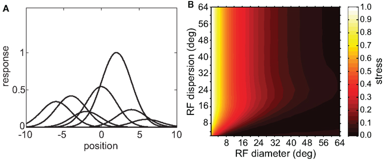
Figure 10. Spatial representations recovered from an inhomogeneous neural population containing neurons tuned to different shape features. (A) Heights of Gaussian spatial tuning curves varied depending on responsiveness of each neuron to the single shape used as a stimulus. Tuning curves are depicted schematically as 1D functions, whereas they were actually 2D Gaussian functions. Peak heights have been normalized so that the tallest peak is equal to 1.0. (B) 3D plot of stress as a function of RF diameter and RF dispersion, using a population with inhomogeneous shape responsiveness. Stimulus configuration was a 16° diameter grid.

For the simulations we varied the spatial tuning curve height for each neuron by multiplying it by a gamma distributed random number. The equation for a gamma probability density function is:

where Γ is the gamma function. The parameters were set to a = 2.0 and b = 0.5, giving a mean value of the multiplicative factor of ab = 1.0. A gamma distribution was chosen because neurophysiological data indicates that the probability distribution of responses in a neural population to a single shape stimulus is right-skewed (Lehky et al., 2005; Franco et al., 2007).

Having thus created a mosaic of cells tuned to different shape features, we proceeded in the same manner as before to examine the representation of space, using one fixed shape as stimulus. The resulting 3D plot of stress as a function of RF diameter and RF dispersion for an inhomogeneous population is shown in Figure 10B. For comparison, the same plot for a homogeneous population under the same stimulus conditions is given in Figure 5B.

Including inhomogeneous shape responsiveness in the population did not degrade the ability to form spatial representations. In fact, for some parameter conditions (small RF dispersion and large RF diameter), the inhomogeneous population had substantially lower stress than the homogeneous population. For many other parameter conditions there was little difference between homogeneous and inhomogeneous populations. There were no conditions under which the inhomogeneous population noticeably underperformed the homogeneous population.

Having considered the effects of stimulus scale on recovered spatial representations in Figures 5 and 8 we then examined stimulus translation. We used a stimulus grid whose diameter was small enough (6°) that it formed fairly accurate low-dimensional representations when centered at fixation (Figure 11A), given the RF parameters chosen (large dispersion, 48°, left column; or small dispersion, 12°, right column; holding RF diameter constant at 12°). Upon translating the stimulus configuration to 4° eccentricity (Figure 11B), the spatial representation remained accurate for the wide RF dispersion, but became highly distorted for the narrow RF dispersion.

FIGURE 11

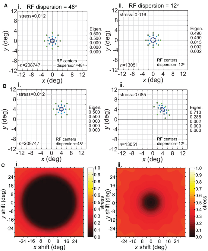
Figure 11. Effect of stimulus translation on the recovered spatial representation: different RF dispersions. Left column: wide RF dispersion (48°). Right column: narrow RF dispersion (12°). (A) Stimulus configuration centered at fixation. (B) Stimulus configuration centered at (4°, 4°). (C) 3D plot of stress as a function of x and y stimulus translation. In all cases, receptive field diameter was 12°, receptive field spacing 0.1°, and the stimulus configuration was a 6° diameter grid.

For the stimulus configuration at 4°, the recovered spatial representation is plotted as centered at 4° in Figure 11B to facilitate comparison with the physical stimulus (this shift in the plot is caused by the Procrustes transform). In reality, because spatial representations are based on distances between population response vectors that result in an intrinsic code (relative positions), the center of the representation is not tied to a particular coordinate; the center location is undefined (see also translated stimuli in Sereno and Lehky, 2011). Because we are just extracting relative positions, representation of the stimulus configuration is position invariant at a population level (within limits described next).

Stress is plotted as a function of stimulus translation in Figure 11C for the two RF dispersion values. The plots show a central region around fixation where spatial representations of Euclidean physical space are highly accurate. The diameter of that central region roughly corresponds to RF dispersion. Again, as we are using intrinsic coding in this model, different positions of the stimulus configuration within the central region cannot be distinguished. In other words, the central region defines an area of positional invariance, where the recovered stimulus configuration does not change. Distortion of the recovered stimulus configuration starts to increase as the edge of the stimulus configuration passes beyond the region containing RF centers (despite the fact that the RFs themselves extend far past the RF centers). With this additional distortion, the recovered spatial configuration changes shape in different parts of the visual field, and positional invariance is lost in the periphery. Overall the representation of space is non-Euclidean due to the “distortion” in the periphery, but is approximately Euclidean (given large enough RF diameter) for a variable region around fixation, dependent on RF dispersion.

While we see in Figure 11C that RF dispersion had a critical effect on the size of the region of positional invariance, RF diameter was not a major factor determining invariance. Figure 12C shows stress plotted as a function of stimulus translation for small RF diameter (4°, left column) and large RF diameter (24°, right column), holding RF dispersion constant at 48°. The central region of invariance was essentially the same diameter for both RF diameters.

FIGURE 12

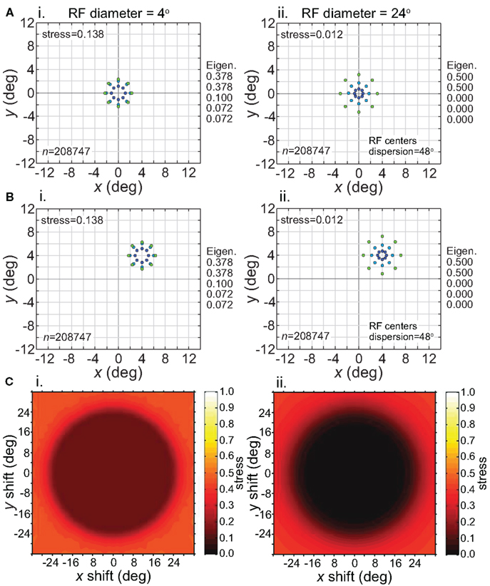
Figure 12. Effect of stimulus translation on the recovered spatial representation: different RF diameters. Left column: small RF diameter (4°). Right column: large RF diameter (24°). (A) Spatial representation recovered from the model with stimulus configuration centered at fixation. (B) Spatial representation recovered from the model with stimulus configuration centered at (4°,4°). (C) 3D plot of stress as a function of x and y stimulus translation. In all cases, receptive field dispersion was 24°, receptive field spacing 0.1°, and the stimulus configuration was a 6° diameter grid.

Although the size of the invariance window was not strongly affected by RF diameter, the level of distortion within the window was diameter-dependent. Small RFs led to higher distortion in the recovered spatial representation within the window (Figure 12, left column). However, despite the higher distortion, the representation remained invariant because the relative positions of points remained unchanged as the stimulus configuration was shifted about. Thus we see, comparing left and right columns in Figure 12, that the issues of accurate representation and invariant representation are dissociable.

The intrinsic nature of the spatial representation extracted by the model during stimulus translation is made explicit in Figure 13. This figure corresponds to the left column of Figure 11 (wide RF dispersion), with the translation occurring inside the window of invariance. The first row in Figure 13 indicates the physical stimulus configuration, centered at [0°, 0°] (left column) or translated to [4°, 4°] (right column). The second row shows the MDS outputs at the two stimulus locations. Because MDS is only recovering relative positions of stimulus points, information about absolute position has been lost. The representations for the centered and translated stimuli are essentially identical. In other words, the representations are position invariant. The third row shows the output from the Procrustes transform. Here the MDS output has been transformed to maximize congruence with the physical stimulus configuration, a procedure that allows us to quantify how well the relative positions of the stimulus points have been recovered.

FIGURE 13

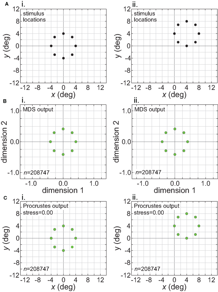
Figure 13. Translation of stimulus configuration (large RF dispersion). This corresponds to the conditions in left column of Figure 11, inside central invariant area. Left column: stimulus configuration centered at fixation [0°, 0°]. Right column: stimulus configuration centered at [4°, 4°]. (A) Physical stimulus configuration, a ring of points 8° in diameter. (B) Output of multidimensional scaling procedure. (C) Procrustes transform of MDS output. Receptive field diameter was 24°, receptive field dispersion was 48°, and receptive field spacing was 0.1°.

While Figure 13 shows the effects of stimulus translation inside the window of invariance, Figure 14 shows what happens when translation goes beyond that window. Figure 14 corresponds to the situation in the right column of Figure 11 (narrow RF dispersion). In the MDS output (Figure 14B), information about absolute position has been lost. However, in this case the loss of absolute position information did not lead to a positionally-invariant representation. Shifting the stimulus location caused secondary non-invariances by changing the scale of the representation and also distorting relative positions of points within the stimulus configuration (“shape”). (The change in scale of the MDS output could have been removed by normalizing the distance matrix in the MDS procedure to have some fixed mean value, which we did not do.) Thus we see here that the absence of absolute positonal information is necessary but not sufficient for positional invariance.

FIGURE 14

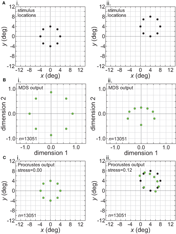
Figure 14. Translation of stimulus configuration (small RF dispersion). This corresponds to conditions in right column of Figure 11, outside central invariant area. Left column: stimulus configuration centered at fixation [0°, 0°]. Right column: stimulus configuration centered at [4°, 4°]. (A) Physical stimulus configuration, a ring of points 8° in diameter. (B) Output of multidimensional scaling procedure. (C) Procrustes transform of MDS output. Green dots indicate recovered spatial configuration, black dots indicate original physical spatial configuration. (Black dots are obscured in left Procrustes panel.) Receptive field diameter was 24°, receptive field dispersion was 12°, and receptive field spacing was 0.1°.

Noise is a ubiquitous feature of neural responses. The effect of noise on recovered spatial representations was examined using noise that was either correlated (correlation coefficient = 1.0) or uncorrelated (correlation coefficient = 0.0) amongst cells in the population. The noise had two components, one being background noise independent of the level of neural activity and the other proportional to neural activity. The overall equation for the noise-corrupted response r_n was:

where r was the deterministic response (with range 0.0–1.0) and N(0, σ) was normally distributed noise with mean zero and standard deviation σ. The results are shown in Figure 15. Correlated noise had absolutely no effect. That is as expected because perturbing two neural response vectors in exactly the same way does not affect the distance between them, and therefore does not affect recovered stimulus positions under the MDS analysis we are using. Uncorrelated noise increased distortion in the recovered spatial representation. The increased distortion was not primarily due to random jitter in the recovered positions (although there was some of that), but rather increased signal spreading into the third dimension at larger stimulus eccentricities, mimicking the effect of a smaller RF size. It appears that the chief effect of uncorrelated noise is to reduce the effective RF diameter in the population. Uncorrelated noise also produced negative eigenvalues in the MDS output, indicating that the recovered spatial locations could not be represented within a Euclidean space with complete accuracy.

FIGURE 15

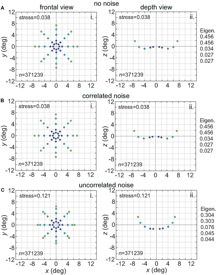
Figure 15. Effect of noise on recovered spatial representations. Left column: frontal view. Right column: depth view. (A) Noise free neurons (B) Neurons with correlated noise (correlation coefficient = 1.0). (C) Neurons with uncorrelated noise (correlation coefficient = 0.0). Receptive field diameter was 64°, receptive field dispersion was 48°, and receptive field spacing was 0.1°.

We also looked at the effects of adding an inhibitory surround to the spatial tuning curves of the RFs. Instead of having Gaussian tuning curves, we used DOG (Eq. 3; Figure 16). This large change in the RF profile allowed us to examine if the results were highly sensitive to our general assumption that RFs were Gaussian. Adding the inhibitory surround had little effect on the spatial representation formed by the population model, making the representation slightly less accurate (higher stress) for populations with smaller RF diameter. The primary determinant of the quality of the spatial representation remained the RF size, and not the presence or absence of suppressive regions in the RF.

FIGURE 16

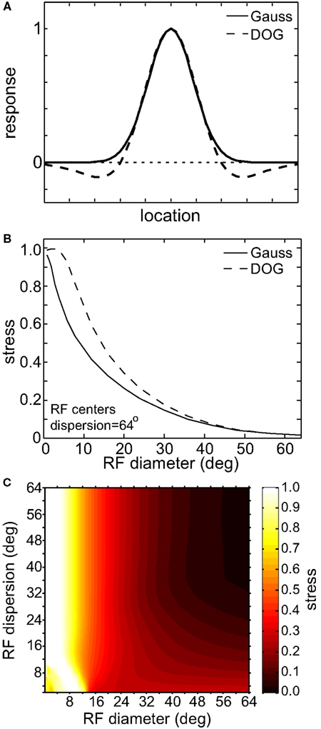
Figure 16. Effect of inhibitory surround within receptive fields on the accuracy of low-dimensional spatial representations. (A) Spatial profiles of two receptive field types. These represent slices through what where actually 2D circularly symmetric receptive fields. (B) 2D plot of stress as a function of receptive field diameter, using both Gaussian and Difference of Gaussians (DOG) receptive fields. RF dispersion was 48°. (C) 3D plot of stress as a function RF diameter and RF dispersion using DOG receptive fields. Compare to Figure 5B, where we used Gaussian receptive fields. In both (B) and (C) RF spacing was 0.1° and stimulus configuration was a 16° grid.

In many visual areas RF diameter increases as a function of eccentricity (Hubel and Wiesel, 1974; Gattass and Gross, 1981; Gattass et al., 1981, 1988; Van Essen et al., 1984; Albright and Desimone, 1987; Boussaoud et al., 1991; Ben Hamed et al., 2001; Motter, 2009). We added this feature to one variant of the model (Figure 17A), making RF diameter increase linearly with eccentricity as has generally been observed in the literature:

where σ₀ was the space constant defining RF diameter (Eq. 1) at the foveal region, E was eccentricity in degrees, and a was the slope of the eccentricity function, set equal to 1.0. Although in reality the slope varies with brain area (appearing to increase the further one gets from striate cortex, Gross et al., 1993), the value we chose was within the range reported in the literature. When comparing constant and eccentricity-dependent RFs we made both their RF diameters equal at the foveal region.

FIGURE 17

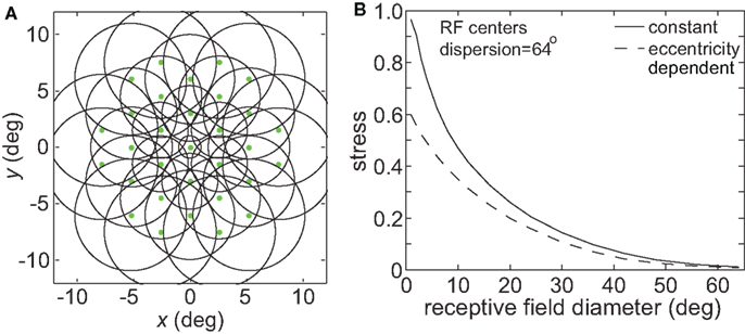
Figure 17. Effect of variable receptive field diameter on accuracy of low-dimensional spatial representations. (A) Neural population with receptive field diameters increasing linearly as a function of eccentricity. Green dots represent receptive field centers and circles represent one space constant of 2D Gaussian receptive fields. Diagram indicates receptive field configuration schematically for easy visualization, and does not match RF parameters used in simulations. (B) Stress as a function receptive field diameter, for both constant and variable diameter receptive fields. For the variable diameters plot, x-axis value is the foveal RF diameter, with that diameter increasing with slope 1.0 as a function of eccentricity. RF spacing was 0.1° and the stimulus configuration was a 16° diameter grid.

Making RF size eccentricity-dependent did lead to some improvement in the accuracy of spatial representations especially for smaller RF diameter (decreased stress between the physical stimulus configuration and the recovered configuration; Figure 17B). However, the behavior of the model essentially remained the same in a qualitative sense, without causing a major change in the shape of the stress vs. RF diameter curve. Given that we already know spatial representations improve when using larger RFs (Figure 3), and that stimuli located at larger eccentricities are the most difficult to accurately incorporate within a spatial representation (Figure 8), it is not surprising that larger RFs in the periphery improve the spatial accuracy achieved by the neural population, especially for populations/areas that have small RFs near the fovea.

Another variation in RF shape was to make them anisotropic rather than circularly symmetric, as biological RFs are never perfectly circular. For our simulations we used elliptical RFs (Eq. 2), oriented vertically with the long axis double the length of the short axis (32° × 16°, Figure 18A). The spatial representation recovered from a population with such RFs is shown is Figure 18B. Stress was higher with elliptical RFs, compared to stress for circular fields having the same mean RF diameter (24°; see Figure 3B). Inspection of Figure 18B shows the nature of this increased distortion: stimulus configurations that are physically circular were represented as elliptical, especially at small eccentricities. The vertical/horizontal anisotropies in this representation of space matched those of the underlying RFs.

FIGURE 18

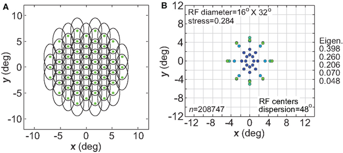
Figure 18. Effect of anisotropic receptive fields on spatial representations. (A) Neural population with elliptical receptive fields. (B) Spatial representation produced by elliptical receptive fields. Space constants of the Gaussian receptive fields were 16° in the x-direction and 32° in the y-direction. RF spacing was 0.1° and the stimulus configuration was a 16° diameter grid.

Receptive fields associated with a single cerebral hemisphere cover primarily the contralateral half of the visual field. We examined the effect this might have on spatial representations by confining RF centers of the model to one hemifield (Figure 19A). Results are given in Figure 19B. As would be expected, the representation of space was highly skewed toward the hemifield covered by the RFs. This skewing may be slightly overstated by the model, as our distribution of RF centers was strictly confined to one side whereas biologically there is some scatter to the other side, especially in higher visual areas. One effect of the skewing was to produce a vertical/horizontal anisotropy in the representation of space, resembling that seen in Figure 18. Thus we see that anisotropic spatial representations can result from either an anisotropic RF shape (Figure 18) or an anisotropic distribution of RFs centers (Figure 19).

FIGURE 19

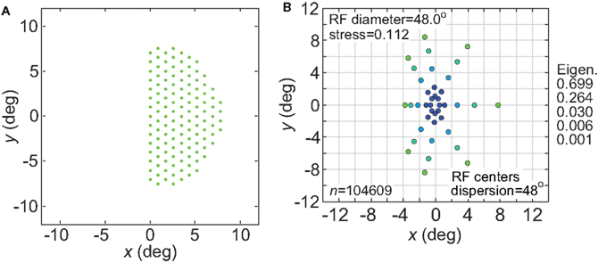
Figure 19. Effect of confining receptive field centers to one visual hemifield. (A) Green dots represent configuration of receptive field centers responding to right visual field stimuli (left cerebral hemisphere). (B) Representation of space produced by the hemifield receptive field geometry. RF spacing was 0.1° and the stimulus configuration was a 16° diameter grid.

So far we have primarily used a regular hexagonal array of RF centers (as in Figure 1). Figure 20 examines the effects of placing the RF centers at random locations, following either a uniform distribution or a Gaussian distribution (the Gaussian distribution mimicked the greater concentration of RFs observed in the central representations of visual cortex). The results show virtually no difference between using a regular array of RF centers and a uniform random distribution (plot lines overlapping). Accuracy of the spatial representations was reduced slightly using a Gaussian random distribution of RF centers. Using a Gaussian distribution appeared to have an effect equivalent to a slight reduction in the RF dispersion.

FIGURE 20

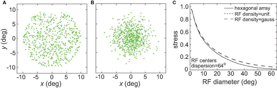
Figure 20. (A) Effect of random placement of receptive field centers, rather than on a hexagonal grid. Two random distributions were examined: uniform and Gaussian. (A) Example uniform distribution of RF centers. (B) Example Gaussian distribution of RF centers. (C) Stress as a function of RF diameter, for regular hexagonal RF array as well as the two random distributions. The curves for the hexagonal array arrangement and the uniform distribution are almost identical and appear superimposed.

The spatial representations developed above were based on presenting one stimulus point at a time from the stimulus configuration, and then comparing population activities as that point was moved to different locations. In Figure 21 we explore interactions between two stimulus points presented simultaneously, with linear summation of responses within each RF. The space was mapped out as one stimulus point remained at a fixed location and a second point moved to different positions within a grid.

FIGURE 21

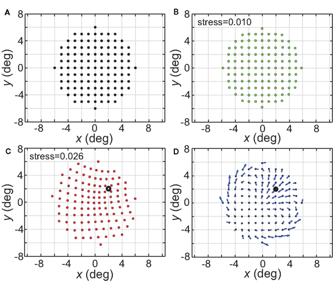
Figure 21. Distortion of spatial representation in vicinity of a fixed stimulus point. (A) Configuration of stimulus points in physical space. It consisted of a 6° × 6° square grid of points at 1° intervals. (B) Spatial representation of stimulus configuration recovered by neural model. Neural space was mapped presenting one stimulus point at a time, as was done in all previous cases described here. (C) Spatial representation when two stimulus points were presented simultaneously. One stimulus point was held fixed at location (2°, 2°), indicated by the black dot. Neural space was then mapped with a second point presented at different positions along the square grid. RF diameter was 48°, RF dispersion was 48°, and receptive field spacing was 0.1°. (D) Differences between panels (B) and (C) indicate spatial distortions caused by two-point interactions. Blue arrows indicate magnitude and direction of difference for each stimulus point.

The physical stimulus configuration is given in Figure 21A, consisting of a circular grid of stimulus locations. The spatial representation recovered from population activity using the usual single-point procedure is shown in Figure 21B, for a set of population parameters providing a highly accurate spatial recovery (RF diameter = 32°; RF dispersion = 64°). The next panel (Figure 21C) shows how the simultaneous presence of a second fixed stimulus point (marked by a large open dot) warped the representation of space.

Figure 21D indicates, by the use of arrows for each point, the magnitude (length) and direction (angle) of these spatial distortions (two stimuli versus one stimulus), demonstrating both attraction and repulsion in the apparent relative positions of the two points. Overall, the representation of space in a region around the points becomes contracted with a general shift toward the spatial center of the population (not the center of the stimuli). If the second stimulus is off-center (e.g., Figure 21C) the distortion is maximal near this stimulus and mostly occurs within the hemifield containing the stimulus, with little change spilling into the space directly opposite. If the second stimulus is placed at the spatial center of the population (not shown), the contraction toward the center occurs from all directions. Replacing the hexagonal grid of RF centers with either a uniform random distribution or Gaussian random distribution leads to similar two-point spatial warping.

Discussion

We have developed a population coding model of visual space based on an intrinsic representation of stimulus locations, and explored how the resulting representation of space is affected by the RF characteristics of the neural population implementing it. An intrinsic representation means that stimulus locations are defined relative to each other, and not relative to an external coordinate frame (Lappin and Craft, 2000). In their psychophysical study, Lappin and Craft (2000) concluded that visual space is encoded in an intrinsic manner. Our model is an intrinsic representation as a consequence of the fact that there are no “labeled lines”: the reconstruction of space is based entirely on neural firing rates without labels attached to each firing rate indicating RF properties (position, size, shape) of the neuron.

Spatial representations based on extrinsic coding are firmly anchored to a particular external coordinate system (external to the stimuli, which may include a coordinate system defined by a grid of RFs). The problem in that case is to find ways of making the representation invariant (with respect to scale, translation, and rotation) for particular situations, such as for some aspects of object recognition. On the other hand spatial representations based on intrinsic coding, which only specify relative positions, are inherently invariant. The problem now is the opposite: to generate non-invariant representations (representations tied to a particular physical location, orientation, etc.) as the need arises.

We suggest that one primary need for non-invariant visual representations arise from interacting with the physical world, such as required in visuomotor control of saccades, reaching, or grasping. Non-invariance can be effected by making sensory representations of space and motor representations of space consistent with each other through learning (e.g., Fuchs and Wallman, 1998; Krakauer et al., 2000). Neural representations of space could be arbitrarily scaled, rotated and reflected provided that, through learning, visual maps and motor control maps become aligned in appropriate cortical areas such that visual guidance leads to successful motor performance. Connecting perceptual representation to action in the world serves to tie the representation to some external frame of reference (similar in purpose to the Procrustes transform formalism that was used as a tool in the model to quantify congruence between the extracted representation and the original physical stimulus configuration).

Although intrinsic coding leads to invariant representations, our simulations found that the characteristics of the neural substrate placed limits on such invariance. For example, in Figure 11 we saw that translational invariance for low-dimensional representations was limited to a region around fixation, whose size was defined by RF dispersion. In general, throughout various simulations, we found that undistorted low-dimensional representations of physical space were confined to an area around fixation whose size depended on the RF characteristics of the population. We give the name “Euclidean window” to the limited region of space around fixation where low-dimensional representation appears to be approximately Euclidean and various invariances hold. It has also been called, within a psychological context, the “Newtonian oasis” (Heelan, 1983; Arnheim, 2004).

Note that positional invariance here refers to maintaining relative positions within a stimulus configuration unchanged when the configuration is presented at different locations in the visual field. The same term, positional invariance, has also been used in the past to describe unchanged rank order of responses to different shapes at different positions (Ito et al., 1995; Janssen et al., 2008). We suggest that this concept might better be described instead as invariant feature-selectivity across stimulus position.

In this study we have been interested in identifying conditions that lead to accurate representations of physical space when those representations are confined to 3D manifolds within a high-dimensional neural response space. We suggest here that making the representation of visual space dimensionally isomorphic with 3D physical space allows a more efficient interface between perceptual representations and motor representations for visuomotor control (where the motor representations control action in the physical world). This is a variant of the idea of Soechting and Flanders (1992) that maintaining common representational formats in different parts of the brain might facilitate exchange of information. In addition, Edelman and Intrator (1997) have argued that low-dimensional visual representations in general make many perceptual problems more tractable by reflecting the low-dimensional nature of the real world. In general, given the principle that the simplest model or description of the world is to be preferred (see Hempel, 1966; Popper, 2002; re Ockham’s razor), it can be argued that a low-dimensional representation fits that criterion by offering mathematically the most parsimonious description. Even though low-dimensional and high-dimensional representations of space may be equivalent in terms of information content, formatting the same information in different ways within a neural population can lead to changes in the nature, speed, and efficiency of the processing that is supported, as was pointed out by Kosslyn (1986). Seung and Lee (2000) provide a general discussion of the possible importance to perceptual processing of low-dimensional manifolds within high-dimensional neural response spaces.

By suggesting that in some cases spatial representations may be dimensionally isomorphic with physical space, we are proposing an isomorphism that is abstract and functional (a low-dimensional manifold embedded within a high-dimensional neural response space), rather than a structural isomorphism where 3D space is literally represented by a 3D grid of neurons in the brain (see Lehar, 2003 for a discussion of functional versus structural isomorphism). Representations lying on such a functional manifold retain neighborhood spatial relations without any requirement for actually reducing the high-dimensionality of responses of the embedding neural population.

Implicit in the suggestion above that low-dimensional representations of space may be critical for efficient visuomotor control, is the possibility that the dimensionality of space may be dissimilar in different cortical regions. In particular, low-dimensional spatial representations may occur within the dorsal visual stream, which is associated with the representation of space for the control of action (Ungerleider and Mishkin, 1982; Goodale and Milner, 1992), while the ventral visual stream may not be constrained to such a low-dimensional representation (or may be operating in a reference frame, perhaps allocentric, that appears high-dimensional when mapped retinotopically). Evidence for this is presented in the accompanying paper (Sereno and Lehky, 2011), which reports low-dimensional spatial representation in a dorsal structure (lateral intraparietal cortex) and higher-dimensional representation in a ventral structure (anterior inferotemporal cortex, AIT).

The idea that spatial representations may be different in different cortical areas finds support in our simulations. Having a model allowed us to examine how the nature of the spatial representation is determined by neural population characteristics, and we indeed found that the representation of space was strongly affected by those characteristics.

In the model, RF diameter was an important determinant of the capability of neural populations to accurately encode visual space within a low-dimensional manifold. There are several dozen visually responsive cortical areas (Felleman and Van Essen, 1991), and RF diameters differ widely amongst those areas. The smallest RFs are located in striate cortex, where they are typically a small fraction of a degree across (Hubel and Wiesel, 1977; Kagan et al., 2002). RF diameter progressively increases as one ascends the hierarchy of visual areas. At the upper levels of the hierarchy, median RF diameters are around 10° in either the ventral visual pathway (Op de Beeck and Vogels, 2000) or dorsal visual pathway (Ben Hamed et al., 2001). It is difficult to give a definite number for RF diameter because different labs have used different conditions or definitions and at higher cortical stages RF size appears to be substantially modulated by stimulus conditions (Op de Beeck and Vogels, 2000; Rolls et al., 2003).

Based on our modeling, these different visual areas should have different capabilities for forming accurate low-dimensional representations of space. Using intrinsic spatial coding, as we did for this model, populations with small RFs can only form highly distorted spatial representations. If the RFs are sufficiently small, the distortion increases to the extent that not only are the metrics of space warped, but even the topological ordering of points in space become scrambled (Figure 3C). In extrastriate areas with larger RF sizes, the capacity to represent visual space with high accuracy improves.

For the intrinsic spatial coding used here we found that large RFs produced the most accurate representations. The opposite would hold true if spatial coding were extrinsic. If the response of each cell were somehow labeled with the retinotopic coordinates of that cell (plus other RF properties), then striate cortex, with very small RFs would produce the most precise global spatial maps, while higher visual areas with larger RFs would have the poorest spatial representations. Without such an assumption of labeled lines, although responses of small RFs are sensitive to slight changes in stimulus position, there is only a limited ability to attach a location to those responses within the context of a large global map. To accomplish that global spatial mapping with unlabeled neural responses, the RFs themselves must be spread out globally.

In addition to RF size, another important parameter identified by the modeling was the dispersion of RF centers. While it is widely appreciated that RF size varies in different visual areas, it is perhaps less well known that the dispersion of RF centers also varies. Striate cortex has its RF centers spread out over the broadest range, with substantial numbers extending out to 30° or 40° from the foveal representation (Gattass et al., 1981; Van Essen et al., 1984). At the other extreme, the most narrowly dispersed RF centers are found in AIT, where they are almost entirely confined to within 3°–4° of the fovea (Tovée et al., 1994; Op de Beeck and Vogels, 2000). Between those two values, we have RF center dispersions for V2 (Gattass et al., 1981), V3 (Gattass et al., 1988), V4 (Gattass et al., 1988; Motter, 2009), posterior inferotemporal (Boussaoud et al., 1991), and moving dorsally, area MT (Gattass and Gross, 1981) as well as LIP (Ben Hamed et al., 2001), with dispersion values falling in the range of 10–20° from the fovea.

The modeling results indicate that the most accurate low-dimensional spatial representations occur for stimulus configurations placed inside the central region of the visual field where RF centers are located. Although that might appear to give an advantage to the area with the broadest dispersion, namely striate cortex, RF diameters in striate cortex are so small that even the best spatial reconstructions near fixation are very poor. The higher extrastriate areas, with their larger RFs, are better able to support accurate global spatial representations. However because the dispersions of RF centers are more narrowly focused in those areas, low distortion representations are restricted to more central areas of the visual field (within 10–20° of fovea). AIT in particular, because its RF centers are severely confined to within 4°, would have the most constricted region of accurate spatial representations, confined to the foveal and parafoveal regions. In cases where good spatial representations are restricted to central vision, it would then be necessary to build up accurate large-scale metric maps of space by a sequential process, integrating information in memory over multiple saccades.

Using the terminology of Kosslyn et al. (1992), cortical areas with large RF diameter and wide RF dispersion implement a coordinate representation of Euclidean physical space in a metrically accurate manner. Cortical areas with somewhat smaller RF diameter, but particularly with narrow RF dispersion, represent space in a qualitative categorical manner, retaining neighborhood relations such as ordering (a point is to the left or right of another, for example). Kosslyn et al. (1992), using back-propagation modeling, noted a similar relation between RF diameter and coordinate/categorical representations of space that we have found here using MDS, with larger RFs providing the most accurate representation of space.

Our model investigated position invariant encoding at the population level rather than single-cell level, using intrinsic encoding of space to extract relational structures within a configuration of stimulus positions. This is a different approach from that taken by some computational models of object recognition, which look for invariance in single-cell properties and postulate large-diameter RFs as a mechanism for position invariant recognition (e.g., Riesenhuber and Poggio, 2000; Serre et al., 2007). Instead of invariance occurring at the single neuron level, we suggest that invariant coding may be a population property, involving conservation of relationships amongst neural activities in a population.

In our model, a central region of translational invariance around fixation was defined primarily by the dispersion of RF centers in the population (Figure 11). As discussed earlier, accurate spatial representation of the stimulus configuration within a low-dimensional manifold required both large RF diameter and wide RF dispersion. On the other hand, invariant spatial representation for translation depended on wide RF dispersion, but, significantly, did not require large RF diameter. Accuracy and invariance are two properties of spatial representations that can be dissociated. As objects are, to some extent, defined by the spatial configuration of their parts, these results may also relate to issues in object recognition.

Consistent with the limited range of translational invariance seen in the model, psychophysical data also shows limitations in position invariance during object recognition tasks (Kravitz et al., 2008). Furthermore, other models of object recognition emphasize the need to retain some degree of positional information (rather than positional invariance) in order to maintain the separate identities of multiple objects within a scene (Roudi and Treves, 2008; Li et al., 2009).

Moreover, physiological data indicates position information is present in the responses of cells with large RFs, even in the ventral stream (Op de Beeck and Vogels, 2000; Lehky et al., 2008; Sereno and Lehky, 2011). Recent human fMRI studies also show modulation of responses in the ventral stream by spatial information (Sayres and Grill-Spector, 2008; Kravitz et al., 2010). Such spatial selectivity is a necessary consequence of having Gaussian RFs, as data in those studies indicate is the case. The presence of large RFs cannot be taken in itself as evidence that spatial information is being lost.

As was mentioned above, RF dispersion is broader in LIP (Ben Hamed et al., 2001) than in AIT (Tovée et al., 1994; Op de Beeck and Vogels, 2000). Under our model, we would predict greater translational invariance in LIP. Applying the same population coding analysis as used here, physiological data in the accompanying paper (Sereno and Lehky, 2011) suggests that such is indeed the case.

Although we have framed the discussion here in terms of stimulus “points,” the same methods can be used to recover the positions of more complex shapes. For example, in the accompanying non-human primate paper, we present simple geometric objects (circles, triangles, etc.) at different positions while recording single-cell responses. Using identical MDS methods for these monkey data as used in the model, we recover the position of those objects. Visual neurons are selective to both location and shape, and population coding for both occurs together. In this model we focus on location coding while ignoring the shape aspect of responses.

Psychophysical investigations have found large distortions in the perception of space, such that the global geometric structure of visual space appears to be non-Euclidean (Suppes, 1977; Indow, 2004; Wagner, 2006). This is shown, for example, by measurements of the apparent frontoparallel plane (AFPP) horopter (Herring, 1879/1942; Helmholtz, 1910/1962; Ogle, 1962; Foley, 1966; Musatov, 1976). If a horizontal array of vertical rods is placed along an objective frontoparallel plane, they appear to curve away from the observer. If the positions of the rods are adjusted such that they subjectively appear on a frontoparallel plane, the array physically curves inward. This is an indication of a curved visual space (in this case with a hyperbolic or Bolyai–Lobachevsky geometry), rather than a Euclidean space. A seminal model of hyperbolic visual space was developed by Luneberg (1947). Although most experimental work and modeling has involved binocular viewing conditions, the finding that perceptual space is non-Euclidean extends to monocular vision as well (Koenderink et al., 2010).

The modeling presented here also produces an apparent curvature of space when presented with stimuli within a frontoparallel plane (right column panels, Figures 3 and 4). Curvature of space in the model was a product of RF characteristics (RF diameter and dispersion of RF centers) in the encoding neural population. With large enough RFs, the modeling shows a region around fixation where a Euclidean representation of space appears to hold to a close approximation (what was called above the “Euclidean window”), with non-Euclidean distortions becoming greater as stimulus configurations extend to larger eccentricities.

In the model, viewing these distortions in the representation of visual space as curvature in depth depends on giving a spatial interpretation to the third dimension of the MDS output. That would be analogous to the way that the first two MDS dimensions were given a spatial interpretation as the x- and y-directions in the frontoparallel plane. All dimensions produced by MDS are mathematical abstractions and must be provided with physical interpretations as part of the modeling process. The spread of signals into the fourth MDS dimension and higher was interpreted as misplacement of points (distortion) within the three spatial dimensions.

Horizontal–vertical anisotropies in the representation of space occurred under two conditions within the model. First, it occurred if the RFs themselves were anisotropic (non-circular; Figure 18). Second, it occurred if the distribution of RF centers were anisotropic, with a strong bias toward a contralateral placement of the RF centers (Figure 19). Non-circular RFs have previously been suggested as an explanation for anisotropic perception of space seen in psychophysical data (McGraw and Whitaker, 1999). Here we suggest, in addition to that, a second possibility, namely, the distribution of RF centers. One consequence of vertical/horizontal anisotropy is to make the eigenvalues for the first two dimensions markedly unequal, as shown in Figures 18 and 19. A similar inequality was found in eigenvalues from MDS analysis of psychophysical spatial data (Indow, 1968), providing additional evidence that human vision is indeed anisotropic. It is interesting to note that anisotropy was also found in the eigenvalues from an identical MDS analysis of physiological spatial data in monkeys (see Sereno and Lehky, 2011). Some forms of amblyopia involve abnormal distortions of visual space with an exaggerated degree of anisotropy (Lagrès and Sireteanu, 1991). Under the modeling here, that might be attributed to disturbances in the RF organization in extrastriate cortex.

In the laboratory, it is often critical to reduce the complexity of input, for example to a single stimulus, to begin to understand how the visual system operates. While most of our manipulations used a single stimulus presentation, we did also briefly consider two-stimuli interactions. Our model showed that the representation of space was warped by the simultaneous presentation of two stimuli (Figure 21). Such warping of space in the region near a visual stimulus has been observed psychophysically (Badcock and Westheimer, 1985a,b; Greene and Brown, 1995; Ruda, 1998), and it is possible that visual crowding effects (Levi, 2008) may also be due to spatial distortion caused by multiple stimuli. More generally, it has long been recognized that there are spatial interactions with simultaneous multiple stimuli, both in behavioral studies (Sereno and Kosslyn, 1991; Sereno and Sereno, 1999) as well as physiological studies (such as response modulation beyond the classical RF, Allman et al., 1985; Knierem and Van Essen, 1992).

We modeled the effects of two stimuli by linearly summing the responses to the stimuli within each RF, with no excitatory or inhibitory influences between different neurons. The source of spatial interactions was therefore quite different than normally postulated in the neurophysiology literature. Rather than having such interactions mediated by horizontal synaptic connections between neurons (e.g., Das and Gilbert, 1999), they occurred here purely as the result of population activity amongst non-interacting neurons. While lateral connections are likely to be one important aspect of this issue, the model raises the possibility that population coding effects, not apparent at the single-cell level, also contribute to spatial interactions observed perceptually. Although linear summation of responses from multiple stimuli within a single RF may not be biophysically realistic, it is sufficient to demonstrate the principle. See Sereno and colleagues (Patel et al., 2010; Sereno et al., 2010) for more elaborate dynamical modeling of spatial interactions amongst multiple stimuli.

While we presented the two stimuli simultaneously, the timing between two stimuli may be critical. For example, both behavioral (e.g., Posner and Cohen, 1984) and physiological studies (Bell et al., 2004) show that changes in stimulus timing can produce either reflexive facilitation or inhibition depending on the degree of asynchrony. Moreover, the shapes of the two stimuli (same or different) affect these reflexive spatial interactions (Patel et al., 2010; Sereno et al., 2010). In addition, it is possible that instead of having two stimuli physically present (i.e., reflexive attention), voluntary attention directed at a point may have a similar effect, so that voluntary attention might lead to similar distortions in spatial representations. Thus, the inclusions of dynamic neuronal properties, lateral interactions, multiple stimuli, feature tuning, as well as voluntary attentional conditions are potential areas for future development of a more complete spatial model.

Conflict of Interest Statement

The authors declare that the research was conducted in the absence of any commercial or financial relationships that could be construed as a potential conflict of interest.

Acknowledgments

The research was supported by a grant from the NSF 0924636. We thank Saumil Patel, Margaret Sereno, and Anthony Wright for comments on the manuscript.

References

Albright, T. D., and Desimone, R. (1987). Local precision of visuotopic organization in the middle temporal area (MT) of the macaque. Exp. Brain Res. 65, 582–592.

Pubmed Abstract | Pubmed Full Text

Allman, J. M., Miezin, F. M., and McGuiness, E. (1985). Stimulus specific responses from beyond the classical receptive field: neurophysiological mechanisms for local-global comparisons in visual neurons. Annu. Rev. Neurosci. 8, 407–430.

Pubmed Abstract | Pubmed Full Text

Arnheim, R. (2004). Art and Visual Perception: A Psychology of the Creative Eye. Berkeley: University of California Press.

Averbeck, B. B., Latham, P. E., and Pouget, A. (2006). Neural correlations, population coding and computation. Nat. Rev. Neurosci. 7, 358–366.

Pubmed Abstract | Pubmed Full Text

Badcock, D. R., and Westheimer, G. (1985a). Spatial location and hyperacuity: flank position within the centre and surround zones. Spat. Vis. 1, 3–11.

CrossRef Full Text

Badcock, D. R., and Westheimer, G. (1985b). Spatial location and hyperacuity: the centre/surround localization contribution function has two substrates. Vision Res. 25, 1259–1267.

Bell, A. H., Fecteau, J. H., and Munoz, D. P. (2004). Using auditory and visual stimuli to investigate the behavioral and neuronal consequences of reflexive covert orienting. J. Neurophysiol. 91, 2172–2184.

Pubmed Abstract | Pubmed Full Text | CrossRef Full Text

Ben Hamed, S., Duhamel, J.-R., Bremmer, F., and Graf, W. (2001). Representation of the visual field in the lateral intraparietal area of macaque monkeys: a quantitative receptive field analysis. Exp. Brain Res. 140, 127–144.

Pubmed Abstract | Pubmed Full Text | CrossRef Full Text

Borg, I., and Groenen, P. (1997). Modern multidimensional scaling: theory and applications. New York: Springer.

Boussaoud, D., Desimone, R., and Ungerleider, L. G. (1991). Visual topography of area TEO in the macaque. J. Comp. Neurol. 306, 554–575.

Pubmed Abstract | Pubmed Full Text

Curto, C., and Itskov, V. (2008). Cell groups reveal structure of stimulus space. PLoS Comput. Biol. 4, e1000205. doi: 10.1371/journal.pcbi.1000205.

Pubmed Abstract | Pubmed Full Text | CrossRef Full Text

Cutzu, F., and Edelman, S. (1996). Faithful representation of similarities among three-dimensional shapes in human vision. Proc. Natl. Acad. Sci. U.S.A. 93, 12046–12050.

Pubmed Abstract | Pubmed Full Text

Das, A., and Gilbert, C. D. (1999). Topography of contextual modulations mediated by short-range interactions in primary visual cortex. Nature 399, 655–661.

Pubmed Abstract | Pubmed Full Text | CrossRef Full Text

Deneve, S., Latham, P. E., and Pouget, A. (1999). Reading population codes: a neural implementation of ideal observers. Nat. Neurosci. 2, 740–745.

Pubmed Abstract | Pubmed Full Text

Edelman, S. (1999). Representation and Recognition in Vision. Cambridge, MA: MIT Press.

Edelman, S., and Duvdevani-Bar, S. (1997). A model of visual recognition and categorization. Philos. Trans. R. Soc. Lond., B, Biol. Sci. 352, 1191–1202.

Pubmed Abstract | Pubmed Full Text

Edelman, S., and Intrator, N. (1997). “Learning as extraction of low-dimensional representations,” in Mechanisms of Perceptual Learning, eds D. Medin, R. Goldstone, and P. Schyns (New York: Academic Press), 353–380.

Felleman, D. J., and Van Essen, D. C. (1991). Distributed hierarchical processing in the primate cerebral cortex. Cereb. Cortex 1, 1–47.

Pubmed Abstract | Pubmed Full Text

Foley, J. M. (1966). Locus of perceived equidistance as a function of viewing distance. J. Opt. Soc. Am. 56, 822–827.

Pubmed Abstract | Pubmed Full Text

Franco, L., Rolls, E. T., Aggelopoulos, N. C., and Jerez, J. M. (2007). Neuronal selectivity, population sparseness, and ergodicity in the inferior temporal visual cortex. Biol. Cybern. 96, 547–560.

Pubmed Abstract | Pubmed Full Text | CrossRef Full Text

Fuchs, A. F., and Wallman, J. (1998). Saccadic gain modification: visual error drives motor adaptation. J. Neurophysiol. 80, 2405–2416.

Pubmed Abstract | Pubmed Full Text

Gattass, R., and Gross, C. G. (1981). Visual topography of striate projection zone (MT) in posterior superior temporal sulcus of the macaque. J. Neurophysiol. 46, 621–638.

Pubmed Abstract | Pubmed Full Text

Gattass, R., Gross, C. G., and Sandell, J. H. (1981). Visual topography of V2 in the macaque. J. Comp. Neurol. 201, 519–539.

Pubmed Abstract | Pubmed Full Text

Gattass, R., Sousa, A. P., and Gross, C. G. (1988). Visuotopic organization and extent of V3 and V4 of the macaque. J. Neurosci. 8, 1831–1845.

Pubmed Abstract | Pubmed Full Text

Goodale, M. A., and Milner, A. D. (1992). Separate visual pathways for perception and action. Trends Neurosci. 15, 20–25.

Pubmed Abstract | Pubmed Full Text | CrossRef Full Text

Greene, H. H., and Brown, J. M. (1995). The effect of nearby luminance contrast polarity on color boundary localization. Vision Res. 35, 2767–2771.

Pubmed Abstract | Pubmed Full Text | CrossRef Full Text

Gross, C. G., Rodman, H. R., Gochin, P. M., and Colombo, M. W. (1993). “Inferior temporal cortex as a pattern recognition device,” in Proceedings of the Third Annual NEC Research Symposium, ed. E. Baum (Philadelphia: SIAM), 44–73.

Heelan, P. A. (1983). Space-perception and the Philosophy of Science. Berkeley: University of California Press.

Helmholtz, H. L. F. v. (1910/1962). Treatise on Physiological Optics. New York: Dover.

Hempel, C. G. (1966). Philosophy of Natural Science. Englewood Cliffs, NJ: Prentice-Hall.

Pubmed Abstract | Pubmed Full Text

Herring, E. (1879/1942). Spatial Sense and the Movement of the Eye. Baltimore, MD: American Academy of Optometry.

Hori, E., Tabuchi, E., Matsumura, N., Tamura, R., Eifuku, S., Endo, S., Nishijo, H., and Ono, T. (2003). Representation of place by monkey hippocampal neurons in real and virtual translocation. Hippocampus 13, 190–196.

Pubmed Abstract | Pubmed Full Text | CrossRef Full Text

Hubel, D. H., and Wiesel, T. N. (1974). Uniformity of monkey striate cortex: a parallel relationship between field size, scatter, and magnification factor. J. Comp. Neurol. 158, 295–305.

Pubmed Abstract | Pubmed Full Text

Hubel, D. H., and Wiesel, T. N. (1977). Ferrier lecture. Functional architecture of macaque monkey visual cortex. Proc. R. Soc. Lond. B, Biol. Sci. 198, 1–59.

Indow, T. (1968). Multidimensional mapping of visual space with real and simulated stars. Percept. Psychophys. 3, 45–53.

Indow, T. (1982). An approach to geometry of visual space with no a priori mapping functions: multidimensional mapping according to Riemannian metrics. J. Math. Psychol. 26, 204–236.

Indow, T. (2004). The Global Structure of Visual Space. Singapore: World Scientific.

Ito, M., Tamura, H., Fujita, I., and Tanaka, K. (1995). Size and position invariance of neuronal responses in monkey inferotemporal cortex. J. Neurophysiol. 73, 218–226.

Pubmed Abstract | Pubmed Full Text

Izenman, A. J. (2008). Modern Multivariate Statistical Techniques: Regression, Classification, and Manifold Learning. New York: Springer.

Janssen, P., Srivastava, S., Ombelet, S., and Orban, G. A. (2008). Coding of shape and position in macaque lateral intraparietal area. J. Neurosci. 28, 6679–6690.

Pubmed Abstract | Pubmed Full Text | CrossRef Full Text

Jazayeri, M., and Movshon, J. A. (2006). Optimal representation of sensory information by neural populations. Nat. Neurosci. 9, 690–696.

Pubmed Abstract | Pubmed Full Text

Kagan, I., Gur, M., and Snodderly, D. M. (2002). Spatial organization of receptive fields of V1 neurons of alert monkeys: comparison with responses to gratings. J. Neurophysiol. 88, 2557–2574.

Pubmed Abstract | Pubmed Full Text | CrossRef Full Text

Kant, I. (1781/1999). Critique of Pure Reason. Cambridge: Cambridge University Press.

Kiani, R., Esteky, H., Mirpour, K., and Tanaka, K. (2007). Object category structure in response patterns of neuronal population in monkey inferior temporal cortex. J. Neurophysiol. 97, 4296–4309.

Pubmed Abstract | Pubmed Full Text | CrossRef Full Text

Knierem, J. J., and Van Essen, D. C. (1992). Neuronal responses to static texture patterns in area V1 of the alert macaque monkey. J. Neurophysiol. 67, 961–980.

Pubmed Abstract | Pubmed Full Text

Koenderink, J. J., Albertazzi, L., van Doorn, A. J., van Ee, R., van de Grind, W. A., Kappers, A. M. L., Lappin, J. S., Norman, J. F., Oomes, A. H. J., te Pas, S. P., Phillips, F., Pont, S. C., Richards, W. A., Todd, J. T., Verstraten, F. A. J., and de Vries, S. (2010). Does monocular visual space contain planes? Acta Psychol. (Amst.) 134, 40–47.

Pubmed Abstract | Pubmed Full Text

Köhler, W. (1992). Gestalt Psychology: An Introduction to New Concepts in Modern Psychology. New York: Liveright.

Kosslyn, S. M. (1986). Image and Mind. Cambridge, MA: MIT Press.

Pubmed Abstract | Pubmed Full Text

Kosslyn, S. M., Chabris, C. F., Marsolek, C. J., and Koenig, O. (1992). Categorical versus coordinate spatial relations: computational analyses and computer simulations. J. Exp. Psychol. Hum. Percept. Perform. 18, 562–577.

Pubmed Abstract | Pubmed Full Text

Krakauer, J. W., Pine, Z. M., Ghilardi, M.-F., and Ghez, C. (2000). Learning of visuomotor transformations for vectorial planning of reaching trajectories. J. Neurosci. 20, 8916–8924.

Pubmed Abstract | Pubmed Full Text

Kravitz, D. J., Kriegeskorte, N., and Baker, C. I. (2010). High-level visual object representations are constrained by position. Cereb. Cortex 20, 2916–2925.

Pubmed Abstract | Pubmed Full Text | CrossRef Full Text

Kravitz, D. J., Vinson, L. D., and Baker, C. I. (2008). How position dependent is visual object recognition? Trends Cogn. Sci. 12, 114–122.

Pubmed Abstract | Pubmed Full Text

Kriegeskorte, N., Mur, M., Ruff, D. A., Kiani, R., Bodurka, J., Esteky, H., Tanaka, K., and Bandettini, P. A. (2008). Matching categorical object representations in inferior temporal cortex of man and monkey. Neuron 60, 1126–1141.

Pubmed Abstract | Pubmed Full Text | CrossRef Full Text

Lagrès, W.-D., and Sireteanu, R. (1991). Two-dimensional spatial distortions in human strabismic amblyopia. Vision Res. 31, 1271–1288.

CrossRef Full Text

Lappin, J. S., and Craft, W. D. (2000). Foundations of spatial vision: from retinal images to perceived shapes. Psychol. Rev. 107, 6–38.

Pubmed Abstract | Pubmed Full Text

Lee, J. A., and Verleysen, M. (2007). Nonlinear Dimensionality Reduction. New York: Springer.

Lehar, S. (2003). Gestalt isomorphism and the primacy of subjective conscious experience: a Gestalt bubble model. Behav. Brain Sci. 26, 375–408.

Pubmed Abstract | Pubmed Full Text

Lehky, S. R., Peng, X., McAdams, C. J., and Sereno, A. B. (2008). Spatial modulation of primate inferotemporal responses by eye position. PLoS ONE 3, e3492. doi: 10.1371/journal.pone.0003492.

Pubmed Abstract | Pubmed Full Text | CrossRef Full Text

Lehky, S. R., and Sejnowski, T. J. (1990). Neural model of stereoacuity and depth interpolation based on a distributed representation of stereo disparity. J. Neurosci. 10, 2281–2299.

Pubmed Abstract | Pubmed Full Text

Lehky, S. R., Sejnowski, T. J., and Desimone, R. (2005). Selectivity and sparseness in the responses of striate complex cells. Vision Res. 45, 57–73.

Pubmed Abstract | Pubmed Full Text | CrossRef Full Text

Lehky, S. R., and Sereno, A. B. (2007). Comparison of shape encoding in primate dorsal and ventral visual pathways. J. Neurophysiol. 97, 307–319.

Pubmed Abstract | Pubmed Full Text | CrossRef Full Text

Levi, D. M. (2008). Crowding – an essential bottleneck for object recognition: a mini-review. Vision Res. 48, 635–654.

Pubmed Abstract | Pubmed Full Text | CrossRef Full Text

Li, N., Cox, D. D., Zoccolan, D., and DiCarlo, J. J. (2009). What response properties do individual neurons need to underlie position and clutter “invariant” object recognition? J. Neurophysiol. 102, 360–376.

Pubmed Abstract | Pubmed Full Text | CrossRef Full Text

Luneberg, R. K. (1947). Mathematical Analysis of Binocular Vision. Princeton: Princeton University Press.

McGraw, P. V., and Whitaker, D. (1999). Perceptual distortions in the neural representation of visual space. Exp. Brain Res. 125, 122–128.

Pubmed Abstract | Pubmed Full Text | CrossRef Full Text

Motter, B. C. (2009). Central V4 receptive fields are scaled by the V1 cortical magnification and correspond to a constant-sized sampling of the V1 surface. J. Neurosci. 29, 5749–5757.

Pubmed Abstract | Pubmed Full Text

Motter, B. C., and Mountcastle, V. B. (1981). The functional properties of the light-sensitive neurons of the posterior parietal cortex studied in waking monkeys: foveal sparing and opponent vector organization. J. Neurosci. 1, 3–26.

Pubmed Abstract | Pubmed Full Text

Musatov, V. I. (1976). An experimental study of geometric properties of visual space. Vision Res. 16, 1061–1069.

Pubmed Abstract | Pubmed Full Text | CrossRef Full Text

Ogle, K. N. (1962). “The optical spatial sense,” in The Eye, Vol. 4, ed. H. Davson (New York: Academic Press), 211–417.

Op de Beeck, H., and Vogels, R. (2000). Spatial sensitivity of macaque inferior temporal neurons. J. Comp. Neurol. 426, 505–518.

Pubmed Abstract | Pubmed Full Text

Op de Beeck, H., Wagemans, J., and Vogels, R. (2001). Inferotemporal neurons represent low-dimensional configurations of parameterized shapes. Nat. Neurosci. 4, 1244–1252.

Pubmed Abstract | Pubmed Full Text

Oram, M. W., Földiák, P., Perrett, D. I., and Sengpiel, F. (1998). The ‘Ideal Homunculus’: decoding neural population signals. Trends Neurosci. 21, 259–265.

Pubmed Abstract | Pubmed Full Text | CrossRef Full Text

Patel, S. S., Peng, X., and Sereno, A. B. (2010). Shape effects on reflexive spatial selective attention and a plausible neurophysiological model. Vision Res. 50, 1235–1248.

Pubmed Abstract | Pubmed Full Text | CrossRef Full Text

Popper, K. (2002). The Logic of Scientific Discovery, 2nd Edn. New York: Routledge.

Posner, M. I., and Cohen, Y. A. (1984). “Components of visual orienting,” in Attention and Performance X, eds H. Bouma and D. G. Bouhuis (Hillsdale, NJ: Laurence Earlbaum and Associates), 531–556.

Pouget, A., Dayan, P., and Zemel, R. (2000). Information processing with population codes. Nat. Rev. Neurosci. 1, 125–132.

Pubmed Abstract | Pubmed Full Text

Quian Quiroga, R., and Panzeri, S. (2009). Extracting information from neuronal populations: information theory and decoding approaches. Nat. Rev. Neurosci. 10, 173–185.

Pubmed Abstract | Pubmed Full Text

Riesenhuber, M., and Poggio, T. (2000). Models of object recognition. Nat. Neurosci. 3(Suppl.), 1199–1204.

Pubmed Abstract | Pubmed Full Text | CrossRef Full Text

Rolls, E. T., Aggelopoulos, N. C., and Zheng, F. (2003). The receptive fields of inferior temporal cortex neurons in natural scenes. J. Neurosci. 23, 339–348.

Pubmed Abstract | Pubmed Full Text

Roudi, Y., and Treves, A. (2008). Representing where along with what information in a model of a cortical patch. PLoS Comput. Biol. 4, e1000012. doi: 10.1371/journal.pcbi.1000012.

Pubmed Abstract | Pubmed Full Text | CrossRef Full Text

Ruda, H. (1998). The warped geometry of visual space near a line assessed using a hyperacuity displacement task. Spat. Vis. 11, 401–419.

Pubmed Abstract | Pubmed Full Text

Sayres, R., and Grill-Spector, K. (2008). Relating retinotopic and object-selective responses in human lateral occipital cortex. J. Neurophysiol. 100, 249–267.

Pubmed Abstract | Pubmed Full Text | CrossRef Full Text

Sereno, A. B., and Kosslyn, S. M. (1991). Discrimination within and between hemifields: a new constraint on theories of attention. Neuropsychologia 29, 659–675.

Pubmed Abstract | Pubmed Full Text | CrossRef Full Text

Sereno, A. B., and Lehky, S. R. (2011). Population coding of visual space: comparison of spatial representations in the dorsal and ventral visual pathways. Front. Comput. Neurosci. 4:159. doi: 10.3389/fncom.2010.00159

CrossRef Full Text

Sereno, A. B., Lehky, S. R., Patel, S. S., and Peng, X. (2010). “A neurophysiological correlate and model of reflexive spatial attention,” in Advances in Cognitive Science, Vol. 2, eds N. Srinavasan, B. R. Kar, and J. Pandey (New Delhi: Sage Publications), 104–131.

Sereno, M. E., and Sereno, M. I. (1999). 2-D center-surround effects on 3-D structure-from-motion. J. Exp. Psychol. Hum. Percept. Perform. 25, 1834–1854.

Pubmed Abstract | Pubmed Full Text

Serre, T., Krieman, G., Kouh, M., Cadieu, C., Knoblich, U., and Poggio, T. (2007). A quantitative theory of immediate visual recognition. Prog. Brain Res. 165, 33–56.

Pubmed Abstract | Pubmed Full Text | CrossRef Full Text

Seung, H. S., and Lee, D. D. (2000). Cognition. The manifold ways of perception. Science 290, 2268–2269.

Pubmed Abstract | Pubmed Full Text | CrossRef Full Text

Shephard, R. N. (1980). Multidimensional scaling, tree-fitting, and clustering. Science 210, 390–397.

Pubmed Abstract | Pubmed Full Text | CrossRef Full Text

Soechting, J. F., and Flanders, M. (1992). Moving in three-dimensional space: frames of reference, vectors, and coordinate systems. Annu. Rev. Neurosci. 15, 167–191.

Pubmed Abstract | Pubmed Full Text

Sugihara, T., Edelman, S., and Tanaka, K. (1998). Representation of objective similarity among three-dimensional shapes in the monkey. Biol. Cybern. 78, 1–7.

Pubmed Abstract | Pubmed Full Text | CrossRef Full Text

Suppes, P. (1977). Is visual space Euclidean? Synthese 35, 397–421.

CrossRef Full Text

Tovée, M. J., Rolls, E. T., and Azzopardi, P. (1994). Translation invariance in the responses to faces of single neurons in the temporal visual cortical areas of the alert macaque. J. Neurophysiol. 72, 1049–1060.

Toye, R. C. (1986). The effect of viewing position on the perceived layout of space. Percept. Psychophys. 40, 85–92.

Pubmed Abstract | Pubmed Full Text

Ungerleider, L. G., and Mishkin, M. (1982). “Two cortical systems,” in Analysis of Visual Behavior, eds D. J. Ingle, M. A. Goodale, and R. Mansfield (Cambridge, MA: MIT Press), 549–586.

Pubmed Abstract | Pubmed Full Text

Van Essen, D. C., Newsome, W. T., and Maunsell, J. H. (1984). The visual field representation in striate cortex of the macaque monkey: asymmetries, anisotropies, and individual variability. Vision Res. 24, 429–448.

Pubmed Abstract | Pubmed Full Text | CrossRef Full Text

Vogels, R., Biederman, I., Bar, M., and Lorincz, A. (2001). Inferior temporal neurons show greater sensitivity to nonaccidental than to metric shape differences. J. Cogn. Neurosci. 13, 444–453.

Pubmed Abstract | Pubmed Full Text

Wagner, M. (2006). The Geometries of Visual Space. Mahwah, NJ: Lawrence Erlbaum Associates.

Young, G., and Householder, A. S. (1938). Discussion of a set of points in terms of their mutual distances. Psychometrika 3, 19–21.

CrossRef Full Text

Zhang, K., Ginzburg, I., McNaughton, B. L., and Sejnowski, T. J. (1998). Interpreting neuronal population activity by reconstruction: unified framework with application to hippocampal place cells. J. Neurophysiol. 79, 1017–1044.

Pubmed Abstract | Pubmed Full Text