Population coding of visual space: comparison of spatial representations in dorsal and ventral pathways

Introduction

The distinction between ventral and dorsal visual processing has traditionally been described in terms of a “what” vs. “where” dichotomy (Ungerleider and Mishkin, 1982; Ungerleider and Haxby, 1994). In recent years, however, that distinction has become blurred. Shape information has been found in the dorsal stream (Sereno and Maunsell, 1998; Murata et al., 2000; Sereno et al., 2002; Sereno and Amador, 2006; Janssen et al., 2008; Peng et al., 2008), while spatial information has been found in the ventral stream (Op de Beeck and Vogels, 2000; Lehky et al., 2008). It is becoming increasingly apparent that both visual streams are processing shape as well as spatial information. The differences between them appear not to be based on a strict dichotomy between shape and spatial processing, but rather on differences in the nature of shape and spatial information within each visual stream, with encoding of shape and space each geared to the different functionalities of dorsal and ventral processing.

The objective of this study is to characterize differences in the representation of visual space between the two visual streams. Specifically, we compare spatial representations in regions of the brain where we would expect dorsal/ventral differences to be highly salient. Those two structures are anterior inferotemporal cortex (AIT) and lateral intraparietal cortex (LIP), studied under identical task conditions. This complements a previous report in which we demonstrated major differences at a population level of analysis in shape encoding within those two structures (Lehky and Sereno, 2007).

Under one influential framework for understanding dorsal/ventral differences, ventral processing is viewed as oriented toward perception and memory, while dorsal processing is more oriented toward visuomotor control (Ungerleider and Mishkin, 1982; Goodale and Milner, 1992; Jeannerod and Jacob, 2005; Milner and Goodale, 2006). Within that framework, both dorsal and ventral visual structures contain spatial information, but the kind of spatial information differs.

Dorsal spatial representations may be predominantly egocentric (Colby, 1998; Duhamel et al., 1998; Boussaoud and Bremmer, 1999; Snyder, 2000). Egocentric representations involve coordinate frames in which objects or locations are represented relative to the observer (e.g., retinotopic or eye-centered, head-centered, and arm-centered). An egocentric frame would be appropriate for many situations involving real-time guidance of motor actions (saccades, eating, reaching, respectively).

On the other hand, ventral spatial representations may be predominantly allocentric, involving a reference frame external to the viewer (e.g., object-based, scene-based, and world-centered; Booth and Rolls, 1998; Vogels et al., 2001; Kourtzi et al., 2003; Committeri et al., 2004; Aggelopoulos and Rolls, 2005). Such allocentric representations might be used for constructing more abstract models of the world for longer-term use (memory), where knowing a topological or categorical relationship, but not necessarily spatially accurate representation, may be important (e.g., the key that opens the safe is in the top left drawer of the desk). These representations might also be used for conceptual cognitive tasks such as problem solving (for example, planning a route around obstacles to reach a goal).

A possible consequence of the distinction between dorsal egocentric spatial representations and more abstract allocentric representations in the ventral stream has been the observation that dorsal structures appear to provide a more accurate metrical representation of physical space than ventral structures. Geometrical–optical (pictorial) illusions offer one means for studying the neural representation of space (Westheimer, 2008). Some psychophysical studies indicate that dorsal (motor-oriented) representations are less susceptible than ventral representations to various illusions that distort our perceptual judgments within visual awareness (Aglioti et al., 1995; Bridgeman et al., 1997; Haffenden et al., 2001; Ganel et al., 2008; Goodale, 2008); in contrast see (Dassonville and Bala, 2004; Schenk, 2006; Franz and Gegenfurtner, 2008). A higher veridicality in dorsal structures has also been observed using fMRI (Neggers et al., 2006).

The idea of two kinds of spatial representation where one is more veridical is not new (see, e.g., Kosslyn et al., 1989, 1992). As Kosslyn and colleagues pointed out decades ago, computational considerations suggest that different kinds of representation would be useful for different purposes. For guiding action, an accurate “coordinate” spatial representation is necessary. On the other hand, a more “categorical” spatial representation (“right of,” “above,” or “connected to”) is needed to identify objects or scenes. In this case, the brain need not represent the spatial information precisely. In fact, the precise positions of two parts of an object or two objects in a scene that are not relevant can even be potentially harmful (cf. Biederman, 1987; see discussion by Kosslyn et al., 1992).

A major focus of our comparison of dorsal and ventral spatial representations will be on the dimensionality of the representations. Physical space is Euclidean (on spatial scales relevant to this study) and is 3D, and we shall be interested in examining to what extent the neural representation of space is metrically accurate and also dimensionally isomorphic with physical space. A population of neurons encodes spatial information within a high-dimensional neural response space, whose dimensionality is equal to the size of the population. Essentially the question we are asking is whether or not an accurate representation of space can be formed on a 3D manifold embedded within that high-dimensional response space. Possibly the answer may differ for dorsal and ventral pathways. For example, it may be more efficient for dorsal structures to be encoding space in a manner that is dimensionally isomorphic with physical space because they are engaged in visuomotor control of actions occurring within that physical space. On the other hand, ventral structures, possibly engaging with the world in a more abstract manner, may not be under such constraints to form isomorphic representations of space.

The primary analytic approach applied to these data will be statistical dimensionality reduction techniques. While a wide variety of such methods exist (Lee and Verleysen, 2007; Izenman, 2008), we shall use the oldest and most widespread amongst them, multidimensional scaling (MDS; Young and Householder, 1938; Shephard, 1980; Borg and Groenen, 1997). This offers a novel approach to examining dorsal/ventral differences that enables one to quantitatively compare and differentiate spatial representations across neural populations.

Multidimensional scaling has found widespread use in analyzing data related to population coding of shape (Young and Yamane, 1992; Rolls and Tovée, 1995; Sugihara et al., 1998; Edelman, 1999; Op de Beeck et al., 2001; Kayaert et al., 2005; Kiani et al., 2007; Lehky and Sereno, 2007). This will be the first study, to our knowledge, that applies MDS to spatial encoding in visual cortex, although a similar approach has previously been used in monkey hippocampus (Hori et al., 2003), as well as several human psychophysical studies of space perception (Indow, 1968, 1982; Toye, 1986).

The MDS approach to decoding population activity used here assigns spatial interpretations based solely on neural firing rates, without any knowledge of the spatial characteristics of the underlying receptive fields such as peak location, diameter, or shape of the tuning curve. A consequence of our use of unlabeled firing rates is that only relational spatial structures are extracted from population activity (see also, more detailed discussion in Lehky and Sereno, 2011); space is defined in terms of the positions of stimulus points relative to each other. This has been called an intrinsic frame of reference (Lappin and Craft, 2000). We are aware of only one recent model of hippocampal place cells that shares an intrinsic coding of navigational space (Curto and Itskov, 2008), which otherwise takes a different mathematical approach. Our approach is fundamentally different from many models of population coding that assume firing rates are labeled with receptive field parameters (Oram et al., 1998; Zhang et al., 1998; Deneve et al., 1999; Pouget et al., 2000; Averbeck et al., 2006; Jazayeri and Movshon, 2006; Quian Quiroga and Panzeri, 2009). In these models, an extrinsic frame of reference with a grid of receptive fields with known locations and properties is used to define a coordinate system that is external to the stimuli.

This report focuses on experimental data, applying population decoding methods to elucidate and compare the representation of space in ventral and dorsal cortical areas. In the accompanying paper (Lehky and Sereno, 2011) we construct a neural model for the population coding of space, with model output subjected to identical MDS analysis as the monkey physiology data. In that study, by examining how the geometry of the recovered spatial representation is affected by various receptive field parameters (such as receptive field diameters or the spatial distribution of receptive field centers), we hope to gain insight into how differences in spatial encoding we uncover here might arise from known variations in receptive field characteristics.

Materials and Methods

Physiological Preparation

Two male macaque monkeys (Macaca mulatta, 10 kg; Macaca nemestrina, 8 kg) were trained on the behavioral task (described below). A standard scleral search eye coil implanted prior to training monitored eye position. Recording was conducted in both LIP and AIT of each monkey. The chambers for LIP were implanted first and centered 3–5 mm posterior and 10–12 mm lateral, and the chambers for AIT were implanted after recording from LIP and were centered 18 mm anterior and 18–21 mm lateral. Details of the surgical procedures have been described earlier (Lehky and Sereno, 2007). All experimental protocols were approved by the University of Texas, Rutgers University, and Baylor College of Medicine Animal Welfare Committees and were in accordance with the National Institutes of Health Guidelines.

Data Collection and Visual Stimuli

The electrode was advanced while the monkey was performing the task. All encountered cells that could be stably isolated were recorded from extracellularly. Either a platinum/iridium or tungsten microelectrode (1–2 MΩ, Microprobe) was used.

Stimuli were displayed on a 20-inch, 75-Hz CRT monitor with a resolution of 1152 × 864 pixels, placed 65 cm in front of the animal. The monitor subtended a visual angle of 27° height and 36° width. Beyond the monitor was a featureless 45 cm × 60 cm black screen (40° × 54° visual angle), which supported an electromagnetically shielded window in its center through which the animal viewed the monitor. The monkeys viewed the stimuli binocularly. Experiments were conducted in a darkened room.

Prior to the start of data collection for each cell, preliminary testing determined stimulus positions producing a robust response, using a grid of locations over a range of stimulus eccentricities and angles within a polar coordinate system. Preliminary testing also determined the most effective shape stimulus from amongst eight possible shapes (Figure 1A).

FIGURE 1

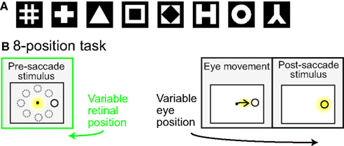
Figure 1. (A) Set of possible stimulus shapes. Preliminary testing of each cell indicated which of these eight shapes was the most effective stimulus for that cell. The most effective shape was then used in all subsequent testing of the spatial properties of the cell. (B) Task design. After the monkey was stably fixating, the stimulus shape appeared randomly at one of eight peripheral locations. The monkey immediately made a saccade to the stimulus. Yellow highlighting indicates eye position and was not present in actual display. For each cell the stimulus shape was always the same, chosen in preliminary testing as the most effective stimulus for that cell. The trial epochs prior to the saccade (marked in green) provided cell responses to the same stimulus at different spatial locations. Data from that epoch was used to evaluate the cells’ spatial selectivity properties.

Spatial selectivity for each cell was tested by presenting the most effective stimulus shape at eight positions. The eight locations all had the same eccentricity, but had different polar angles (Figure 1B). The chosen eccentricity reflected a balance between the two goals of maintaining a robust response and keeping similar stimulus locations for different cells, and did not necessarily maximize responses for each cell. The polar angles of the eight positions covered a full 360° in approximate 45° increments. Stimulus size for different cells ranged from 0.65° to 2.00° (mean: 0.8°), increasing with eccentricity. The size of the fixation window around the central fixation spot was 0.5° (half-width). Other than the stimulus shape or fixation spot, the screen was completely black. All cells that were stable and isolated were included in the raw data set.

Behavioral Task

Each trial began with the presentation of a fixation point at the center of the visual display (Figure 1B). Then a stimulus of the preferred shape for the neuron appeared at one of eight peripheral locations. The animal was required to make an immediate saccade to the stimulus in order to obtain a liquid reward. When the eye position reached the window of the target stimulus, the fixation point was extinguished and the target persisted on the screen for 400 ms. Thus, prior to the saccade, the stimulus was at one of eight possible retinal positions.

Stimuli were presented in block mode. All eight positions were used once in random order to form a block, before being used again in the next block. The number of blocks was minimally 5, but typically 8–12. The monkeys’ performance on this task averaged 92% correct. In addition to this 8-position task, we collected data on a similar 3-position variant of the task. The 3-position task has been described in detail elsewhere (Lehky et al., 2008). Results from the 3-position task will only be outlined briefly below.

Data Analysis

A preliminary analysis using ANOVA was conducted to identify those cells whose response showed a significant main effect of stimulus retinal position. Subsequent analysis focused on those significant cells. The preliminary analysis also included calculation of a spatial selectivity index (SI) for each cell. Selectivity was defined as:

where r_min and r_max are minimum and maximum firing rates over our sample of stimulus locations.

The time period used for these analyses, as well as the MDS analysis described below, started at the onset time of the peripheral stimulus shifted by visual latency, and ended at the time the monkey exited the fixation window also shifted by visual latency. Latency was determined from the pooled peristimulus histogram for all cells in a given cortical area, and defined as the time to half peak height.

Because mean eccentricity of stimulus location in AIT and LIP were not identical, we performed an analysis of covariance (ANCOVA) to take eccentricity into account as a potential confounding factor when comparing various parameters (mean firing rate, mean SI, etc.) for the two cortical areas. Essentially this involved doing a separate linear regression for each cortical area for the parameter of interest vs. eccentricity, and then determining if the two regression lines were significantly different or not.

The core of the analysis focused on use of a longstanding and well-known statistical dimensionality reduction technique, MDS. We used MDS to reduce the number of dimensions for the spatial representation from the size of the population of recorded cells down to a 3D manifold, dimensionally isomorphic with physical space. MDS analysis of neural data involves examining population responses as a whole. Although these data were collected one cell at a time, for purposes of analysis they were treated as if they were simultaneous population responses. We used classical (metric) MDS throughout our analyses. The data used as input to MDS consisted of neural responses to an identical stimulus placed at a limited number of positions (eight, as mentioned above) for each cell. Those stimulus positions differed from cell to cell because they were determined in part by the responsivity of each cell.

Multidimensional scaling requires that stimulus locations for the entire neural population be identical. To meet that mathematical requirement, we used two different approaches, both of which led to similar results. The first approach was to use only a subset of the cells that showed significant spatial selectivity under ANOVA and which had stimulus locations that were tightly clustered, at approximately the same polar angle and within 2° eccentricity of each other. Then, for the purpose of mathematical analysis, the stimuli for different cells were treated as identically located, with that location equal to the average location. The second approach was based on interpolating (and extrapolating) amongst the data points we had. The interpolation approach had the advantage of allowing inclusion of data from a greater number of neurons, as it was not constrained to using only neurons whose stimulus locations fell within the narrow band of overlap. Interpolation also had the further advantage of greater flexibility in examining the consequences of changing the stimulus spatial configuration in various ways (scaling, translation, etc.), not otherwise possible with our data set. For the interpolation approach, all cells were included that showed significant spatial selectivity under ANOVA and which had a stimulus eccentricity of less than 10°. These criteria were the same for AIT and LIP.

The interpolation procedure used the available data points to construct a smooth and continuous spatial response surface for each cell (firing rate as a function of stimulus retinotopic location), using bilinear interpolation (and extrapolation). (This was done using the gridfit.m function by John D’Errico, Matlab File Exchange file ID #8998.) As interpolations were primarily in the radial direction rather than the angular direction, the limited portions of the interpolated response surface used in almost all cases followed a “sunburst” pattern, illustrated in Figure 6 (the exceptions being the translated stimuli in Figures 11aii and 12aii). The central regions of receptive fields were never used in any of our data analysis calculations.

Multidimensional scaling acts as a dimensionality reduction transform on the data. If we have responses from a population of n neurons to a stimulus at a particular spatial location, then that spatial location can be thought of as being represented as a point in n-dimensional space. Data from k spatial locations becomes a set of k points in n-dimensional space (matrix with dimension k × n). The purpose of MDS was to create a low-dimensional approximation (e.g., k points in three dimensions) of the high-dimensional neural representation, an approximation that seeks to preserve relative distances between different points as closely as possible. If such a low-dimensional approximation exists, that means that neural responses are constrained to lie on a low-dimensional manifold (or surface) embedded within the high-dimensional response space. See Seung and Lee (2000) for a discussion of the geometric concept of a manifold applied to cognition. For “low-dimensional approximation” we used three dimensions, because physical space is 3D and we were interested in whether or not space was accurately represented when confined to a manifold that was dimensionally isomorphic with physical space.

Multidimensional scaling was used as a tool to help us evaluate the dimensionality of the representation implicit in population activity. MDS does not cause responses in the data to lie on a low-dimensional manifold, but merely reports if neural responses are constrained in such a manner. No claim is made that the brain ever implements similar algorithms. Within the brain, we believe representations may always be kept distributed across large populations without the need for a dimensionality reduction procedure such as MDS. Nevertheless, the extent to which information can be reduced easily and precisely to the dimensionality of physical space (i.e., 3D) may tell us something about how the information is encoded, and in turn, determine how efficient that coding is for a particular goal (e.g., translation to motor output that must relate to a 3D physical world).

Mathematically, the response of a neural population to a stimulus at a single location is an n-dimensional vector whose elements are the responses of the individual neurons. If we have population data for k stimulus locations then there are k response vectors. The next step in performing the MDS analysis is to calculate the distance between each response vector and all the other response vectors. That leads to a distance matrix, and it is this distance matrix that is the immediate input to the MDS algorithm. It is possible to use a variety of distance metrics when calculating the distance matrix. We used d = 1 − r as our distance metric, where r was the Pearson correlation coefficient between the components of two vectors (x_a1, x_a2, …, x_an) and (x_b1, x_b2, …, x_bn) defining the population responses at two spatial locations a and b. Here each vector component (x_ai or x_bi) represents the average response of the ith neuron to a stimulus at these two particular spatial locations. For a more geometrical interpretation of our distance measure, as correlation between two response vectors increases, the angle between the vectors decreases. Distance was determined entirely by the angles between response vectors and not the vector lengths. The theoretical advantage of using a correlation based distance metric rather than a Euclidean one is that it emphasizes differences in the pattern of relative firing rates within a neural population rather than absolute differences in firing rate (for example, indiscriminately doubling the firing rate of the entire population to all stimuli would show up as a doubling of the difference between stimuli under a Euclidean distance measure but zero change under a correlation measure).

Applying MDS to the distance matrix, we can recover a set of points in 3D space. If we started with a set of neural population responses at eight spatial locations, the MDS output will give us 3D coordinates of those eight spatial locations. Because the original physical stimulus configuration was flat within a frontoparallel plane, the z-coordinate (depth) was constant. Ideally, in the recovered spatial configuration the z-coordinate should also be a constant. In practice, as we shall see, there were distortions such that the recovered configuration was not necessarily flat but did extend into the third dimension.

The MDS output has the same number of dimensions as the input, where dimensionality is equal to the number of neurons in the population. Each dimension in the output is accompanied by an eigenvalue, whose relative magnitude indicates the contribution of that dimension to the representation. It is generally convenient to normalize the sum of all eigenvalues to equal one in order to make their relative contributions more explicit. Dimensions with small eigenvalues can be ignored, with the remaining dimensions providing a good approximation to the original data. Dimensionality reduction is achieved by just retaining those dimensions with the largest eigenvalues. In some cases, as in our data, there are negative eigenvalues. The presence of negative eigenvalues indicates that the neural population could not form a stimulus representation within Euclidean space that was completely distortion-free. The standard procedure in MDS is to ignore negative eigenvalues if they are small relative to positive eigenvalues, just as small positive eigenvalues are ignored during dimensionality reduction. When calculating normalized eigenvalues only positive eigenvalues were included, so that normalized eigenvalues indicated the relative contributions of different dimensions in the best Euclidean approximation for the neural representation of space.

The output of MDS is a set of low-dimensional coordinates defining the locations of stimulus points. These coordinates are extracted from distances between high-dimensional population vectors whose elements are neural firing rates. Hence, the output of MDS (i.e., set of low-dimensional coordinates) is scaled arbitrarily (and not scaled in degrees of visual angle or in centimeters), and may also be rotated and reflected relative to the true spatial configuration of the stimulus points. Thus, MDS recovers the relative spatial configuration of points, and not their absolute positions. This is as expected for any neural representations of space, which can be scaled and rotated arbitrarily relative to physical space (as for example, the world is projected upside down on our retinas with no practical consequences for our ability to operate spatially within the world).

To make a quantitative comparison between physical space and the recovered neural representation of space, it is necessary to rescale the recovered neural space to match the physical space as closely as possible. This is done using a linear transform called a Procrustes transform, which does scaling, rotation, and reflection to match physical space and the neural representation of space as closely as possible, minimizing a function called stress. Stress is the square root of the normalized sum of the squared errors:

In the equation, d_ij is the physical Euclidean distance between stimulus locations i and j, and is the distance recovered from the neural population representation. The denominator normalizes the error by the scale of the distances, with 〈d_ij〉 being the mean of d_ij. The stress measure defined here is the standard goodness-of-fit measure used in Procrustes analysis. A low residual stress after the Procrustes procedure indicates an accurate neural representation of space within a 3D manifold, and high stress indicates a lot of distortion. By calculating stress, spatial representations in different brain areas can be quantitatively compared.

The Procrustes analysis was conducted in three dimensions. When doing these calculations, the z-coordinates of the physical locations were arbitrarily set to zero for all points, as depth was not a variable of the stimulus set. We generally used configurations of points located in a ring (constant eccentricity), at eight positions separated by 45° polar angles, or a grid composed of several concentric rings. To aid the Procrustes transform in aligning the physical and neural spaces, we introduced an asymmetry into this configuration of points by adding a ninth point at a polar angle of 22.5°, although to reduce clutter we do not show that extra point in the plots. The Procrustes transform was used simply as a data analysis tool to obtain a quantitative measure of how good the low-dimensional approximation was, and it is not proposed that the brain carries out such an operation. Unless otherwise noted, when plotting results we show outputs from the Procrustes transform rather than directly from MDS.

A simplified 1D example of the MDS/Procrustes analysis method is given in Figure 2, demonstrating the low-dimensional (in this case, 1D) recovery of stimulus location from a population of seven model neurons with overlapping Gaussian receptive fields. The Procrustes procedure (Figure 2D) linearly transforms the MDS output (Figure 2C) to maximize congruence with the physical stimulus. It is simply a formalism which allows the calculation of stress (distortion) in the relative positions of the three recovered locations (dotted lines) compared to the original physical locations (solid lines).

FIGURE 2

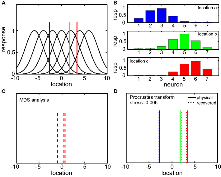
Figure 2. One-dimensional example of decoding population responses to extract stimulus spatial location. (A) Seven neurons whose receptive fields form overlapping Gaussian spatial tuning curves. (In actuality receptive fields would be 2D.) The three colored solid lines mark physical locations of stimuli at x = [−3.80 0.30 1.70]. (B) Population responses to the three stimuli. At each stimulus location, response is given by a seven-component vector, shown in the bar graphs. (C) Recovered relative locations of the three stimuli using multidimensional scaling. Distances between neural response vectors to the three stimuli shown in (B) were quantified and served as input to the MDS procedure. Note that MDS input is based solely on firing rates without knowledge of tuning curve parameters. Three largest normalized eigenvalues associated with the output from MDS were [1 0 0], showing that one dimension accounted for all the variance of the data, as expected for this 1D example. The three locations estimated by MDS were , represented by the three colored dash lines. Inspection of these lines indicates that MDS has recovered the relative locations of the three stimuli. However, as is characteristic of MDS, the procedure failed to recover their absolute positions. (D) Recovered absolute locations of the three stimuli with Procrustes transform. The Procrustes procedure recovered locations x_P = [−2.68 1.83 3.37] by finding the linear transform of that minimizes stress (distortion, see Eq. 2) between the Procrustes estimate and physical location x. That transform is given by x_P = 3.36x_M + 0.84. Residual stress between (dotted lines) and x (solid lines) was 0.006, showing that activity in this population contained a very accurate representation of stimulus locations. That is, that the recovered locations (dotted lines) are only slightly offset from their physical locations (solid lines).

Results

Using the 8-position task, we recorded from 80 cells in AIT and 73 cells in LIP. Histology confirmed that the LIP recording sites were indeed located on the lateral bank of the intraparietal sulcus. AIT cells came predominantly from areas TEav and TEad, with a few located in lateral perirhinal cortex (Brodmann area 36). The histology including these cells has been described in detail previously (Lehky and Sereno, 2007). Mean latency of neural responses under our stimulus conditions was 92 ms in AIT and 70 ms in LIP.

Under analysis of variance (ANOVA), 66.3% (53/80) of the AIT cells showed significant response selectivity for the spatial location of the stimulus. In LIP, 83.6% (61/73) of the cells were spatially selective. These percentages were determined at the p = 0.05 level of significance.

We also analyzed data on a larger sample of cells tested on a 3-position task rather than the 8-position task, and the findings were consistent. The larger sample, including 143 cells from AIT and 122 cells from LIP, included the same cells as used in the 8-position sample plus additional cells. For this sample, 62.2% (89/143) of cells in AIT and 82.8% (101/122) of cells in LIP had significant spatial selectivity. The percentages here are slightly lower than for the 8-position task, perhaps because data from fewer positions were included in the ANOVA. We shall focus below on the 8-position data.

In the 8-position data, for AIT cells with significant location selectivity, mean stimulus eccentricity was 4.3° (range: 2.1–8.0°). For spatially significant LIP cells, mean stimulus eccentricity was 10.7° (range: 7.4–17.6°).

Mean stimulus response over all spatially selective AIT cells was 36 spikes/s, at the most responsive location using the most effective shape stimulus within our set. For LIP, mean stimulus response was 48 spikes/s. An ANCOVA was performed to examine whether mean firing rates were significantly different between AIT and LIP, taking into account differences in stimulus eccentricity as a confounding factor. The analysis showed that brain area (AIT/LIP) was a significant factor affecting firing rate, even when taking into account stimulus eccentricity (p = 0.01). Mean firing rate did tend to decrease slightly as a function of eccentricity, but that effect was not significant (p = 0.08).

The spatial SI (Eq. 1) was calculated for each cell in our sample. Figure 3 presents histograms of the SI values. The mean SI for LIP cells with significant spatial selectivity was 0.71, much higher than the mean value for AIT cells, which was 0.44. That is, LIP cells showed greater modulation of their responses as the stimulus was moved to different locations in the visual field.

FIGURE 3

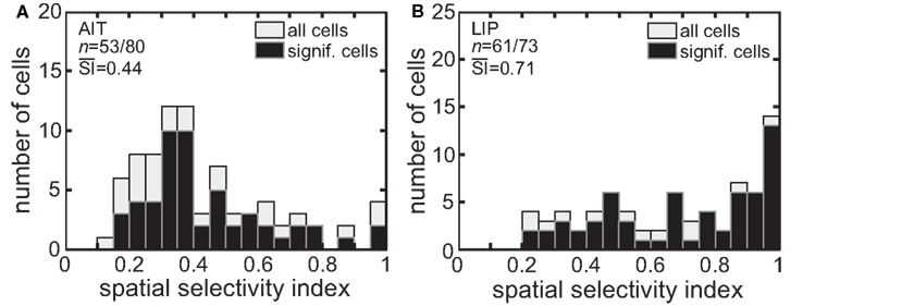
Figure 3. Spatial selectivity index (SI). The SI was calculated for each recorded cell using Eq. 1. The resulting histogram is shown for (A) AIT and (B) LIP. Presented are SI values for all recorded cells as well as for only those cells showing significant spatial selectivity. Mean SI value for spatially significant cells is also shown in each panel.

Again, ANCOVA was performed to see if the difference in the spatial SI between AIT and LIP was significant, taking into account stimulus eccentricity. The difference in spatial selectivity between the two brain areas was highly significant (p < 0.0001). There was no significant effect of stimulus eccentricity on the spatial SI (p = 0.9) in our data.

The time course of visual responses in AIT and LIP (PSTHs) are plotted in Figure 4, averaged over all cells showing significant spatial selectivity under ANOVA. Separate plots indicate average response at the best location and worst location in each brain area. The notable difference between the two brain areas is that on average LIP cells at their least responsive position are suppressed relative to baseline, whereas AIT cells are not. The presence of suppressed responses in LIP serves to increase the dynamic range of responses to stimuli presented at different retinal positions, and may contribute to the higher spatial SI observed in LIP (Figure 3). Interestingly, although suppressed responses in population averages exist in LIP but not AIT for the spatial domain, the opposite occurs for the shape domain. That is, the least effective shape leads to suppression relative to baseline in AIT, but not LIP (Lehky and Sereno, 2007).

FIGURE 4

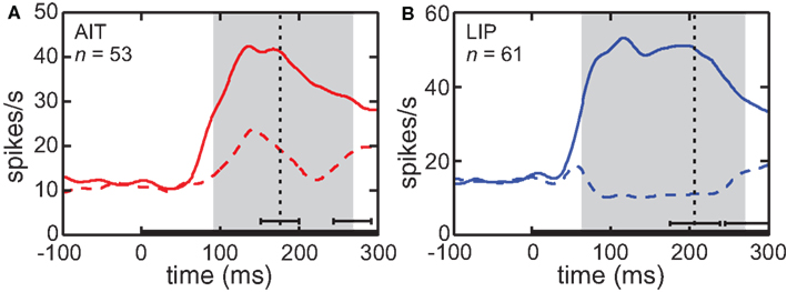
Figure 4. Average time course of responses (PSTH). (A) AIT and (B) LIP. Average time course was calculated over all cells showing significant spatial selectivity, at the most responsive location and least responsive location. Zero time marks presentation of the stimulus in the periphery. Vertical dotted line is the average time of the saccade away from central fixation toward the stimulus. Error bar indicates the standard deviation of the saccade time. The gray region shows the time period used for analyses of the data (ANOVA, SI, and MDS). That period started at stimulus onset and ended at the time of the saccade away from fixation, both times shifted by the average latency of the visual response. Error bar indicates standard deviation of the end of the gray period, due to variations in the time of saccade away from central fixation.

Multidimensional Scaling

MDS comparison of AIT and LIP: no interpolation method

We used a subset of those neurons showing significant spatial selectivity under ANOVA, including only those that had been stimulated at nearly identical locations. The selected cells had stimulus locations within a narrow band of eccentricities (6.0–8.0°) and at the eight standard polar angle positions. For LIP, this included 26 neurons with a mean stimulus eccentricity of 7.44 ± 0.16° SD, and for AIT, 17 neurons with a mean stimulus eccentricity of 6.31 ± 0.70° SD. The stimulus position scatter was small relative to receptive field sizes in those extrastriate areas, and there was not a significant difference in stimulus positions for these subsets of cells recorded in the two cortical areas. As MDS mathematically requires that stimulus locations be identical for all cells, for analysis purposes we treated these tightly clustered stimulus locations (at eight polar angles) as all occurring at their average values for the population, 6.31° (AIT) or 7.44° (LIP) eccentricity.

The MDS/Procrustes procedure previously described was used to recover the spatial representation of the eight locations from population activity. The results are given in Figure 5. It shows that when the high-dimensional population responses are constrained down to a 3D manifold, the recovered spatial representation in LIP more accurately reflects the original physical stimulus configuration than does the AIT representation. The greater accuracy of the LIP representation was reflected in its lower stress value compared to AIT. For LIP, stress = 0.142 ± 0.065 SD while for AIT, stress = 0.541 ± 0.092 SD, with standard deviation estimated by bootstrap resampling of the set of neurons included in the analysis. The difference between stress values for LIP and AIT was significant at p < 0.001 under a t-test, using bootstrap resampling. In addition to the non-linear MDS algorithm, we followed the same procedure using a different dimensionality reduction procedure, principal component analysis (PCA), which is a linear algorithm. Using PCA, spatial distortion was again much lower in LIP, with stress values of 0.182 for LIP and 0.545 for AIT. The PCA method produced very similar stress values to MDS, providing confirmation of the basic results using an independent analysis method. As the PCA method does not allow negative eigenvalues, this is also an indication that negative eigenvalues in the MDS analysis (see below and in MDS Comparison of AIT and LIP: interpolation method) did not play a significant role.

FIGURE 5

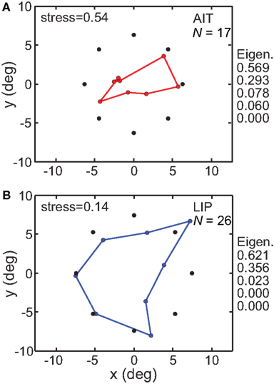
Figure 5. Spatial configuration of stimulus points recovered by multidimensional scaling. MDS analyses were performed on populations whose stimulus locations were tightly clustered around a narrow range of eccentricities. Black dots indicate average location of stimuli, colored dots indicate recovered spatial configuration. (A) AIT, based on 17 neurons with stimuli located at mean 6.31 ± 0.70° SD eccentricity and eight fixed polar angle locations. (B) LIP, based on 26 neurons stimulated at mean 7.44 ± 0.16° SD eccentricity and eight fixed polar angle locations. Also displayed on right are five largest normalized eigenvalues from the MDS analysis. Both stress values and eigenvalues indicate that physical space was more accurately represented in LIP than in AIT, for representations confined to a 3D manifold within the high-dimensional neural response space.

Besides stress, another independent measure of distortion in the recovered low-dimensional spatial representation comes from eigenvalues associated with the MDS analysis. For a neural response vector of dimensionality n (n neurons in the population), we will have n eigenvalues. However, if MDS has been successful in producing an accurate low-dimensional representation of the population response, then only a few of those eigenvalues will be large and most will be zero or close to zero. When all the eigenvalues are normalized such that their sum is 1.0, then the values of the normalized eigenvalues indicate the fraction of variance in the data that is accounted for by each dimension. As the physical stimulus configuration was flat (2D within 3D space), if the neural representation were distortion-free, the normalized eigenvalues would be 0.5 for dimensions 1 and 2, and zero for all other dimensions. (If we had used a 3D stimulus configuration, then ideally the normalized eigenvalues would be 0.333 for the first three dimensions and zero for the others).

Figure 5 shows the five largest eigenvalues associated with the MDS analysis of these data. They indicate greater accuracy in the LIP representation of space than in the AIT representation. For LIP, the eigenvalues were almost entirely confined to the first two dimensions, in keeping with the 2D nature of the stimulus (and more generally in keeping with an accurate low-dimensional representation of space). There was only a small amount of LIP response spreading to the third dimension. For AIT, the first two dimensions accounted for a smaller fraction of the total signal. Spread of the signal into higher dimensions accounts for the “shrinkage” of the recovered AIT points (Figure 5) relative to the physical stimulus.

As physical space is 3D, we interpret the first three MDS dimensions in terms of those physical dimensions. A non-zero value for the third eigenvalue therefore indicates distortion in the representation of the flat stimulus configuration manifesting itself as curvature in depth. Non-zero eigenvalues for dimensions greater than three are interpreted as distortion due to misplacement within 3D space of represented stimulus locations.

The range of eigenvalues for LIP was [0.44 −0.07], and for AIT it was [0.11 −0.01]. The presence of negative eigenvalues indicates that the data could not form a completely accurate representation of stimulus space that was Euclidean. This might have happened because the biological representation of space is intrinsically non-Euclidean as some theoreticians have suggested (Luneberg, 1947; Indow, 2004), or because of noise in the data (see also modeling of noise in accompanying report, Lehky and Sereno, 2011).

MDS comparison of AIT and LIP: interpolation method

Another approach to dealing with the MDS mathematical requirement that stimulus locations for all cells be identical was to perform a spatial interpolation from the available data points before the MDS analysis. An example interpolated response surface is shown in Figure 6, with unused portions blanked out. Interpolated responses at identical locations for all included cells were then used as input to MDS. Included cells were those having significant spatial selectivity under ANOVA and which had a stimulus eccentricity of less than 10°, producing population size n = 53 for AIT and n = 46 for LIP. The input stimulus configuration to MDS then was a ring of eight interpolated responses (at the standard eight polar angles) at a particular constant eccentricity (eccentricities of 2°, 4°, or 8°).

FIGURE 6

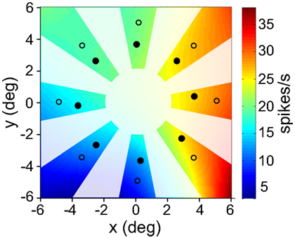
Figure 6. Interpolated/extrapolated responses for an example cell. Eight filled circles indicate locations where data was collected. Based on those points an interpolated surface was fit, providing an estimate of responses over a range of different locations. Only those regions that are not blanked out were used. This procedure was performed for all cells showing significant spatial selectivity under ANOVA. Computing interpolated responses provided the flexibility to perform multidimensional scaling at arbitrary locations across the visual field. Eight open circles are an example set of extrapolated responses used as input to MDS. This example cell was recorded in AIT and had a spatial SI = 0.35.

Recovered spatial configurations are shown in Figure 7. At every eccentricity spatial distortion in LIP was much lower than in AIT, as shown by stress values. This is the same result seen in the previous section where there was no interpolation. Moreover, both methods (with and without interpolation) produced stress values that were quantitatively similar when examined at comparable stimulus eccentricities (Interpolation method: stress_LIP = 0.095, stress_AIT = 0.498, at 8°; No interpolation method: stress_LIP = 0.142, stress_AIT = 0.541, at 7.44° and 6.31° respectively).

FIGURE 7

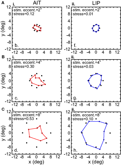
Figure 7. Recovery of the representation of space from neural population activity, for different stimulus eccentricities. Analyses incorporated responses from a local stimulus pattern (one stimulus ring). MDS analysis was based on using interpolated neural responses. Colored dots indicate recovered neural representation of space, and black dots indicate original physical space. Left column. Recovery of spatial representations in AIT at 2°, 4°, and 8° stimulus eccentricity. Larger stimulus eccentricities produce larger stress values (more distorted spatial representations). Right column. Recovery of spatial representations in LIP for stimulus configurations at different stimulus eccentricities.

The level of spatial distortion in Figure 7 increases as a function of stimulus eccentricity for both AIT and LIP. This eccentricity effect is plotted in Figure 8. For MDS, a stress value of 0.1 is a conventional criterion demarcating the border between a “good” low-dimensional approximation and a “poor” one (Borg and Groenen, 1997). By that criterion, LIP maintains accurate low-dimensional representations of space over a wide range of eccentricities, while AIT (extrapolating the curves in Figure 8 to small eccentricities) can only produce accurate spatial representations for stimuli in a limited region close to fixation. As clearly indicated in Figure 8, whatever criterion used, LIP will support more accurate representations of space over a much broader region of the visual field than AIT. This eccentricity effect on the level of spatial distortion is also a feature of the population-coding model presented in the accompanying report (Lehky and Sereno, 2011).

FIGURE 8

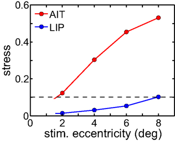
Figure 8. Stress as a function of stimulus eccentricity, for AIT and LIP. Dashed line demarcates 0.1 criterion value for stress indicating a good spatial representation.

Ipsilateral representations were more distorted than contralateral ones in LIP (Figure 9). AIT also showed a similar tendency, but it was not as clear-cut as in LIP. Perhaps that is because there is already high spatial distortion in AIT due to factors other than laterality, and the contralateral/ipsilateral distinction is to some extent being masked. This anisotropy is also a feature recovered from the population-coding model (accompanying report, Lehky and Sereno, 2011) when there are unequal representations of the two visual fields.

FIGURE 9

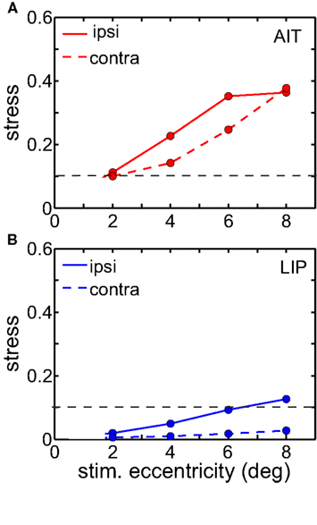
Figure 9. Stress as a function of stimulus eccentricity, for representations of ipsilateral and contralateral space in (A) AIT and (B) LIP. Dashed line demarcates 0.1 criterion value for stress indicating a good spatial representation.

Although Figures 7–9 describe stimuli in terms of eccentricity, an alternative way of describing them is in terms of the extent or diameter of the stimulus locations (i.e., stimulus pattern diameter). A ring of points centered at fixation having a large eccentricity also has a large stimulus pattern diameter. It remains for future experimental investigations to separately examine eccentricity and stimulus extent and test how these variables are influenced by the cortical area being investigated (see also modeling in Lehky and Sereno, 2011).

In addition to using stimulus configurations consisting of a single ring of points (local configuration), we also used a pattern with multiple rings to form a grid of points in a bulls-eye pattern (global configuration). This global stimulus configuration included interpolated stimulus points at 2°, 4°, 6°, and 8° eccentricities, at the standard eight polar angles (Figure 10A).

FIGURE 10

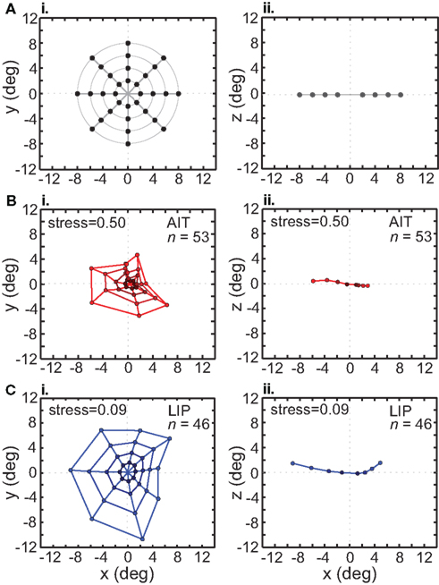
Figure 10. Recovery of the representation of space from neural population activity, using a global (bull’s-eye) stimulus configuration. MDS analysis was performed on interpolated neuronal responses from recorded neurons that had significant spatial selectivity under ANOVA. Left column: plots points from the perspective of the frontoparallel (x–y) plane. Right column: plots points from the perspective of the x–z plane, allowing a view of relative depth of points. The x–z plots are taken along a cross section of space corresponding to the y = 0 axis. (A) Black dots indicate physical configuration of stimulus points. Right column shows that these locations were flat along the frontoparallel plane and did not include a depth component. (B) Configuration of spatial locations recovered from AIT. Coloring becomes darker for points closer to the origin, to aid visualization. (C) Configuration of spatial locations recovered from LIP. Presentation details are the same as in the previous panel. The LIP stress value is lower than in AIT, indicating a more veridical representation of physical space within a 3D manifold.

The grid of points recovered by the MDS/Procrustes analysis for AIT is shown in Figure 10B, and for LIP in Figure 10C. Examination of these plots makes clear that the neural representation of space within a low-dimensional (3D) manifold shows much less distortion in LIP than in AIT. This is confirmed by the lower stress value for LIP (stress = 0.09) than AIT (stress = 0.50). In addition to the x–y plot (frontal plane) in the left column of Figure 10, an x–z plot (depth plane) is presented in the right column, viewed along one cross section of space at the y = 0 axis (precise shapes of these curves will depend on the cross section selected). The x–z plot shows how representation of the flat stimulus configuration is distorted into the third spatial dimension (depth). The range over all eigenvalues for the global stimulus pattern in LIP was [0.62 −0.16], and in AIT, [0.63 −0.21].

Tables 1 and 2 show the normalized eigenvalues produced by the MDS analysis for AIT and LIP, respectively. Each table contains results for the local (single ring) pattern (Figure 7) as well as the global (bulls-eye) stimulus pattern (Figure 10), including only the five largest normalized eigenvalues. Examining normalized LIP eigenvalues in Table 2, we see that the first two dimensions account for all the variance in the data in the smaller local patterns (2°, 4° eccentricity), summing to 1.0. The largest local pattern (8° eccentricity) as well as the global pattern (also 8° maximum eccentricity) had a small amount of distortion into the third dimension, but still captured at least 96% of the variance in the first two dimensions. This dimensionality is consistent with an accurate representation of a flat (2D) stimulus pattern contained implicitly in the high-dimensional population response. However, the two major eigenvalues were unequal, indicating an anisotropic distortion. Such anisotropy was perhaps due to intrinsic ipsilateral/contralateral asymmetries in the visual system (Figure 9).

TABLE 1

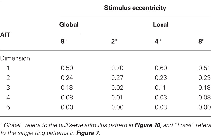
Table 1. Normalized eigenvalues produced by MDS analysis of AIT data, again corresponding to Figures 7 and 10. These indicate the fraction of variance explained by each dimension.

TABLE 2

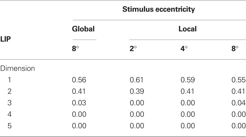
Table 2. Normalized eigenvalues produced by MDS analysis of LIP data.

Moving to the normalized eigenvalues for AIT (Table 1), the first two dimensions accounted for less of the variance than in LIP, indicating a less accurate low-dimensional representation of the 2D stimulus configuration. Even at the smallest stimulus eccentricity (2°) there was sufficient distortion that the data could not be fully represented within two dimensions. As stimulus eccentricity increased, distortion also increased, so that a 2D representation accounted for progressively less of the data.

We examined the effect of translating the stimulus configuration on population responses (Figures 11 and 12), using the interpolation procedure to estimate responses at the shifted locations. The second row in Figures 11 and 12 shows the output of the MDS procedure before [centered at (0° 0°)] and after [centered at (5° 5°)] the translation. Because MDS produces intrinsic coding (recovers relative positions only), information about changes in absolute position associated with the stimulus shift is lost. The third row shows the Procrustes transform of the MDS output. It linearly transforms the MDS output so as to make it as congruent as possible with the stimulus configuration, a formalism that allowed us to quantify how well MDS has recovered relative positions within the stimulus configuration.

FIGURE 11

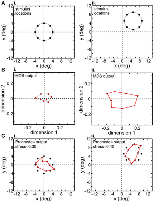
Figure 11. Translation of stimulus configuration in AIT. Left column: stimulus configuration centered at fixation, [0° 0°]. Right column: stimulus configuration centered at [5° 5°]. (A) Physical stimulus configuration, a ring of points 8° in diameter. (B) Output of multidimensional scaling procedure. (C) Procrustes transform of MDS output (colored dots). Black dots indicate physical spatial configuration, for comparison.

FIGURE 12

Figure 12. Translation of stimulus configuration in LIP. All panels analogous with Figure 11.

Although MDS removed information about absolute position when the stimulus configuration was shifted, its output was still not completely translation-invariant. For AIT, comparing the two columns in Figure 11B, there was a change in the overall scale of the MDS output, as well as change in the relative positions of the points. Similar changes were seen in the MDS output for LIP (Figure 12B). To quantify how stimulus translation affected the recovered spatial representation for each cortical area, we compared MDS outputs with the stimulus configuration centered at the [0° 0°] and [5° 5°] locations by calculating stress between those two MDS outputs (from the same cortical area), using the same stress equation as before (Eq. 2). (Here we performed a Procrustes fit between two MDS outputs, whereas before we performed a Procrustes fit between one MDS output and the physical stimulus configuration.) For LIP, this stress was 0.04 and for AIT, it was 0.49. The observation of higher stress (i.e., greater change in output) associated with stimulus translation in AIT was robust for different stimulus translations. By this measure, the spatial representation recovered from population activity shows greater translation invariance in LIP than in AIT.

Discussion

Basic Findings

The majority of neurons in LIP, a dorsal cortical area, as well as AIT, a ventral cortical area, were significantly selective for spatial location. Using identical experimental conditions in both cortical regions, these data show space is represented in both dorsal and ventral visual pathways. These results are consistent with previous neurophysiological spatial studies in AIT (Op de Beeck and Vogels, 2000; Lehky et al., 2008) and LIP (Colby and Duhamel, 1996; Sereno and Amador, 2006). We have previously shown that shape is also represented in both dorsal and ventral pathways (Lehky and Sereno, 2007). Thus, together, these findings suggest that both the ventral and dorsal stream encode information about both space and shape. This is contrary to early formulations of a ventral/dorsal dichotomy in which the ventral pathway was specialized for shape and the dorsal pathway for space (Ungerleider and Mishkin, 1982; Ungerleider and Haxby, 1994).

At the single cell level, both AIT and LIP cells have roughly Gaussian shaped receptive fields, and at the population level both have receptive field distributions that over-represent the central visual field (Op de Beeck and Vogels, 2000; Ben Hamed et al., 2001). In our data, the majority of cells in both AIT and LIP were spatially selective. Yet despite all these similarities, MDS analysis indicated major differences in the representation of space in the two areas.

The results of the MDS analysis showed that physical space could be accurately represented within a 3D manifold in LIP. That was not the case for AIT. In AIT, attempts to represent space on a 3D manifold led to large distortions. All this was indicated, first, from direct examination of the plots resulting from the MDS/Procrustes analysis (Figures 5, 7, and 10), second, from the calculated distortion (stress values) between physical space and the spatial geometry recovered from population activity (also indicated in Figures 5, 7, and 10), and third, from the eigenvalues of the MDS analysis (Tables 1 and 2), which confirmed the stress results using an independent measure. Thus, we show here that the spatial representation implicit within activities of small neural populations recorded under identical task conditions in AIT and LIP are different. Further, in conjunction with our previous findings concerning shape (Lehky and Sereno, 2007), we can now state that although shape and space are encoded in both visual streams, the specific nature of the representations for both shape and space are different in each stream. This is in keeping with the idea of different functions for spatial and shape representations in the two pathways.

Limitations: Number of Locations

The number of locations examined in this study was limited to eight, and did not include depth as a stimulus parameter. The location sample pool was not designed to fully characterize the encoding of space in LIP and AIT neurons but rather to provide a first comparison of spatial response properties in late stages of the two visual pathways. Nevertheless, eight locations that uniformly spanned visual space clearly carried distinct spatial signals, qualifying themselves as reasonable probes to explore the existence of spatial selectivity in LIP and AIT. Further, we demonstrate that even with this limited number of locations in a small population of LIP neurons, we are able to very accurately recover the spatial location of a stimulus. Many studies important in establishing the role of various cortical areas in spatial processing have used a similar restricted set of locations (e.g., Andersen et al., 1985; Funahashi et al., 1989; Rao et al., 1997). In a first comparison of space across ventral and dorsal stream areas, these analyses show, even using a restricted set of locations, striking differences in the organization and encoding of space across the two pathways.

Dimensionality of Spatial Representations and Isomorphism

Results of the MDS analysis are consistent with the idea that LIP spatial responses are low-dimensional, lying on a 3D manifold embedded within a high-dimensional neural responses space. On the other hand, AIT responses are not well described by such a low-dimensional representation.

Accurate neural representation of space on a 3D manifold would make the representation dimensionally isomorphic with 3D physical space. Our data suggests, therefore, that the neural representation of space in LIP is dimensionally isomorphic with physical space, while the AIT spatial representation in general appears not to be. It is important to note that this isomorphism is at an abstract and functional level in which 3D space is represented by a 3D manifold in a high-dimensional space, and not a direct isomorphism in which 3D space is represented by a 3D grid of neurons (see discussion of the distinction between functional and direct isomorphism in the representation of space by Lehar, 2003).

What would be the benefit of a low-dimensional representation of space in LIP? In principle, the spatial information within a population of cells would remain the same whether a high-dimensional or low-dimensional representation were used. The information would just be organized differently. A possible explanation builds on the idea that dorsal structures are engaged in visuomotor control of actions, such as saccades or grasping, whereas ventral structures are engaged in representations for perception and memory (Goodale and Milner, 1992; Goodale and Westwood, 2004). We suggest that for LIP and other dorsal structures, a dimensionally isomorphic 3D perceptual representation of space for visuomotor control may be advantageous in order to more efficiently interface with motor representations that must operate within 3D physical space. As suggested by Soechting and Flanders (1992), keeping the same representational format in a set of cortical areas (dorsal visual and motor cortices, in this case) may enhance the efficiency of communication between them. Seung and Lee (2000) as well Edelman and Intrator (1997) provide general discussions of the possible importance to perceptual processing of low-dimensional manifolds within high-dimensional neural response spaces.

Ventral structures such as AIT are associated with perception rather than motor control, and for those structures isomorphism may be between the neural representation of space and the perceptual experience of space, rather than between neural space and physical space. Psychophysical investigations have found distortions in the perception of space that may mirror the distortions in the neural representation of space found in our data. For example, stimuli lying flat on a frontoparallel plane appear to perceptually curve into the third dimension (Herring, 1879/1942; Helmholtz, 1910/1962; Ogle, 1962; Foley, 1966; Wagner, 2006). Similarly, in our results for the ventral stream (AIT), the neural representation of a flat pattern showed a pronounced component in the third dimension, as indicated by eigenvalues.

Overall, neural representations of space in the dorsal stream (LIP) may be isomorphic with physical space because of our need to physically interact with the world through motor behaviors. On the other hand, AIT and other ventral structures, not engaged in visuomotor control, may not be under the same constraint to form an isomorphic representation of physical space. Rather, ventral structures may form more abstract, categorical representations of space that are not metrically accurate. Distortions in neural representations of space in ventral structures may be isomorphic with a perceptual experience of space that is non-Euclidean, as has been reported by a number of perceptual and modeling investigations (Luneberg, 1947; Musatov, 1976; Suppes, 1977; Heelan, 1983; Indow, 2004).

In general, as pointed out by Kosslyn (1986), reformatting the same information in different ways (low-dimensional vs. high-dimensional representations for the case under consideration here) can lead to changes in the nature, speed, and efficiency of the processing that is supported within neural systems. One must consider how information is used in different cortical areas in order to interpret differences in the dimensionality of spatial representations.

Comparing the Euclidean Window in AIT and LIP

For stimulus configurations centered at fixation, the data indicate that an accurate low-dimensional representation of space is restricted to a very limited region around fixation in AIT, and a much broader region in LIP. As seen in Figures 7 and 8, AIT stress was small (but still greater than LIP) when the eccentricity of the stimulus ring was small, but increased rapidly as the eccentricity increased. In contrast, for LIP, stress remained small at all stimulus ring eccentricities. In other words, for AIT there was a small window around fixation where the neural representation of space is approximately isomorphic with physical space, beyond which spatial distortion quickly became large. For LIP, the window was large. This window, where the neural representation of space is isomorphic with physical space, may be termed the Euclidean window (although within a psychological context it has also been called the “Newtonian oasis” in spatial vision; Heelan, 1983; Arnheim, 2004).

A broad Euclidean window in dorsal visual structures may be appropriate for accurate visual control of a motor action over an extended region. In LIP this action would likely be a saccade but more generally within the dorsal pathway it could include reaching, grasping, or eating. In ventral structures such as AIT, on the other hand, the restriction of a low-distortion spatial representation to a small patch of the visual field (small Euclidean window) would make this area of the brain rather less useful for direct interactions with the physical world. Nevertheless, the categorical spatial representation in AIT could be used to mark the relative locations of different “parts” of an object of limited size (Newell et al., 2005). For scenes containing multiple objects spread out over a moderately wide spatial range, the limited capabilities in AIT would only allow a qualitative, or topological representation of the positions of those objects. While such a topological representation may be sufficient for some applications, it is possible that the formation of a cognitive map or a memory representation of a scene may typically involve pooling information from multiple fixations as the scene is scanned. Previous spatial modeling has also highlighted, as we do here, the importance of a distinction between metrical spatial representations and topological (or categorical) spatial representations (Kosslyn et al., 1992).

Neural Basis for Different Representations of Space in AIT and LIP

Some of the differences between AIT and LIP may be understood in terms of the size and placement of receptive fields. Previous data show that AIT receptive field centers are tightly clustered within 4° of the fovea (Tovée et al., 1994; Op de Beeck and Vogels, 2000), while LIP receptive fields are more broadly dispersed, with many RF centers beyond 10° (Blatt et al., 1990; Ben Hamed et al., 2001). Therefore, the placement of receptive field centers may be one factor leading to more distorted low-dimensional spatial representations in AIT. A population-coding model for the neural representation of space described in the accompanying paper (Lehky and Sereno, 2011) indicates that restricting receptive field centers to a region close to the fovea increases distortion of the representation of space on low-dimensional manifolds, regardless of receptive field diameter (in contrast, cf., Li et al., 2009).

Further, the modeling also indicates that smaller receptive field diameters produce greater spatial distortion in the recovered low-dimensional representation of space (Lehky and Sereno, 2011). That raises the possibility that higher distortion in AIT might also be the result of smaller RF diameter in AIT than in LIP. Comparison of AIT (Op de Beeck and Vogels, 2000) and LIP (Blatt et al., 1990) indicate that AIT RF diameters are smaller [although Ben Hamed et al. (2001) found somewhat smaller LIP diameters than Blatt et al. (1990)]. These RF data measurements are subject to the caveat that they depend on mapping procedures and stimulus conditions, which differed amongst the studies.

Intrinsic Coding of Space

In our analysis, space is coded intrinsically. That is, space is defined in terms of the relative positions of objects located in the space rather than by an externally imposed coordinate system (Lappin and Craft, 2000). The effect of intrinsic coding can be seen in Figures 11B and 12B, showing that the MDS output does not shift when the stimulus configuration is shifted. Note that this loss of absolute positional information occurs at the population level, and not as the immediate result of receptive field characteristics of individual neurons (i.e., large receptive fields).

Intrinsic coding is a result of population representations based purely on neural firing rates, which are not labeled by receptive field characteristics (e.g., RF location, diameter, and shape). This is different from many population-coding models which do assume these RF parameters are known (Oram et al., 1998; Zhang et al., 1998; Deneve et al., 1999; Pouget et al., 2000; Averbeck et al., 2006; Jazayeri and Movshon, 2006; Quian Quiroga and Panzeri, 2009).

Losing information about absolute location but retaining information about relative locations, as occurs for intrinsic coding, can be advantageous in some situations such as object recognition. However there are other situations (e.g., interacting with the world) where it is desirable to have absolute positional information. If one starts with intrinsic coding of relative positions, then creating a representation that contains absolute positional information requires additional processing. This reverses the way the problem is normally posed (e.g., Riesenhuber and Poggio, 1999), where one starts with absolute positional information being available and then must remove it with additional processing.

We suggest that a primary requirement for absolute spatial representations results from the need to interact with the world and have accurate visuomotor control. Absolute spatial representations could be formed by aligning intrinsic perceptual representations with representations for motor control through learning (e.g., Fuchs and Wallman, 1998; Krakauer et al., 2000). Tying perceptual representations to the ability to guide motor actions in the physical world grounds those representations in some external coordinate system. This transformation of the perceptual spatial map in order to make it congruent with a motor spatial map is conceptually equivalent to the Procrustes transform. Different cortical areas might develop different modes of spatial representation (relative or absolute) depending on their functional requirements.

Loss of absolute positional information does not make a representation completely translation-invariant. As we saw in Figures 11B and 12B, although positional information was lost, shifting the stimulus location caused secondary non-invariances by changing the scale of the representation and distorting relative positions of points within the stimulus configuration. Those residual non-invariances may be due to inhomogeneities in population characteristics across the visual field. (Scale non-invariance could be removed by normalizing distance matrices in the MDS analysis to a constant mean value, which we did not do). Our data suggests that LIP is more resistant than AIT to distortions in the relative positions of points induced by stimulus translation. This is consistent with the modeling in the accompanying paper (Lehky and Sereno, 2011) showing that translational invariance is particularly dependent on the breadth of RF center dispersion (something that is known to be more limited in AIT than LIP). Limits to positional invariance in these data are also in accord with psychophysical data indicating that positional invariance in vision may in reality be more limited than widely assumed (Kravitz et al., 2008).

By “positional invariance” we mean that relative positions within a configuration of stimulus points remain unchanged as the configuration is translated across the visual field. The term “positional invariance” has also been used at a single cell level to indicate that the rank order of responses to different shapes remains unchanged at different positions (Ito et al., 1995; Janssen et al., 2008). This very different concept of “positional invariance” might be better described instead as cells having invariant feature-selectivity across stimulus position (see additional discussion below).

Large RF Sizes and Position-Invariance

Large receptive field sizes in AIT have often been interpreted as evidence for “position-invariant” representations of stimuli during object recognition. To the contrary, the present data show that positional information is retained within AIT at both a single cell and population level. Recent fMRI studies corroborate the presence of positional information in ventral visual structures (Sayres and Grill-Spector, 2008; Kravitz et al., 2010). The occurrence of large receptive fields in itself cannot be taken as evidence that spatial information is lost in AIT. In fact, a better way of describing these neurons’ responses is as having invariant feature-selectivity when the stimulus is moved across the receptive field (as indicated by the data of Sary et al., 1993; Ito et al., 1995; Lehky et al., 2008), rather than saying the responses are position-invariant. Our data suggests that the spatial representation recovered from population activity shows greater translation invariance in LIP than in AIT.

Under intrinsic encoding of space, our modeling shows that large receptive fields increase rather than decrease the accuracy of global spatial representations on low-dimensional manifolds (Lehky and Sereno, 2011). The modeling demonstrates not only that large RFs do not result in a loss of relative positional information by the population, but also that small RFs do. A population with sufficiently small receptive fields cannot even recover a topologically consistent spatial representation for spatially extended stimulus configurations.

This relationship between receptive field size and accuracy of the spatial representation holds when using intrinsic encoding of space. The opposite would hold true if extrinsic coding of space were used. For extrinsic coding, small receptive fields, with the crucial addition of labeling information about receptive field properties such as location, diameter, and shape, provide more precise information about spatial positions than large ones. With extrinsic coding, the problem of spatial representation becomes trivial, with just four such spatially overlapping neurons being sufficient to reconstruct 3D visual space through a process of trilateration.

In conclusion, the data presented here support the idea that spatial information is present within neural population responses of both dorsal and ventral visual structures. The nature of that spatial information is quite different in each case, as quantified by a MDS analysis of population responses, probably reflecting the different computational goals within the two visual streams. It remains to be seen if these differences in neural spatial representations between dorsal and ventral visual areas continue into regions of frontal cortex to which they project (e.g., Kennerley and Wallis, 2009).

Conflict of Interest Statement

The authors declare that the research was conducted in the absence of any commercial or financial relationships that could be construed as a potential conflict of interest.

Acknowledgments

This research was supported by grants from the NSF 0924636, the National Alliance for Research on Schizophrenia and Depression (NARSAD), and the J. S. McDonnell Foundation. We thank Saumil Patel, Margaret Sereno, and Anthony Wright for comments on the manuscript, and John Maunsell for assistance with the project.

References

Aggelopoulos, N. C., and Rolls, E. T. (2005). Scene perception: inferior temporal cortex neurons encode the positions of different objects in the scene. Eur. J. Neurosci. 22, 2903–2916.

Pubmed Abstract | Pubmed Full Text

Aglioti, S., Goodale, M. A., and DeSouza, J. F. X. (1995). Size-contrast illusions deceive the eye but not the hand. Curr. Biol. 5, 679–685.

Pubmed Abstract | Pubmed Full Text

Andersen, R. A., Essick, G. K., and Siegel, R. M. (1985). Encoding of spatial location by posterior parietal neurons. Science 230, 456–458.

Pubmed Abstract | Pubmed Full Text | CrossRef Full Text

Arnheim, R. (2004). Art and Visual Perception: A Psychology of the Creative Eye. Berkeley: University of California Press.

Averbeck, B. B., Latham, P. E., and Pouget, A. (2006). Neural correlations, population coding and computation. Nat. Rev. Neurosci. 7, 358–366.

Pubmed Abstract | Pubmed Full Text

Ben Hamed, S., Duhamel, J.-R., Bremmer, F., and Graf, W. (2001). Representation of the visual field in the lateral intraparietal area of macaque monkeys: a quantitative receptive field analysis. Exp. Brain Res. 140, 127–144.

Pubmed Abstract | Pubmed Full Text | CrossRef Full Text

Biederman, I. (1987). Recognition-by-components: a theory of human image understanding. Psychol. Rev. 94, 115–147.

Pubmed Abstract | Pubmed Full Text

Blatt, G. J., Andersen, R. A., and Stoner, G. R. (1990). Visual receptive field organization and cortico-cortical connections of the lateral intraparietal area (area LIP) in the macaque. J. Comp. Neurol. 299, 421–445.

Pubmed Abstract | Pubmed Full Text

Booth, M. C. A., and Rolls, E. T. (1998). View-invariant representations of familiar objects by neurons in the inferior temporal visual cortex. Cereb. Cortex 8, 510–523.

Pubmed Abstract | Pubmed Full Text | CrossRef Full Text

Borg, I., and Groenen, P. (1997). Modern Multidimensional Scaling: Theory and Applications. New York: Springer.

Boussaoud, D., and Bremmer, F. (1999). Gaze effects in the cerebral cortex: reference frames for space coding and action. Exp. Brain Res. 128, 170–180.

Pubmed Abstract | Pubmed Full Text | CrossRef Full Text

Bridgeman, B., Peery, S., and Anand, S. (1997). Interaction of cognitive and sensorimotor maps of visual space. Percept. Psychophys. 59, 456–469.

Pubmed Abstract | Pubmed Full Text

Colby, C. L. (1998). Action-oriented spatial reference frames in cortex. Neuron 20, 15–24.

Pubmed Abstract | Pubmed Full Text | CrossRef Full Text

Colby, C. L., and Duhamel, J.-R. (1996). Spatial representations for action in parietal cortex. Brain Res. Cogn. Brain Res. 5, 105–115.

Pubmed Abstract | Pubmed Full Text

Committeri, G., Galati, G., Paradis, A.-L., Pizzamiglio, L., Berthoz, A., and LeBihan, D. (2004). Reference frames for spatial cognition: different brain areas are involved in viewer-, object-, and landmark-centered judgments about object location. J. Cogn. Neurosci. 16, 1517–1535.

Pubmed Abstract | Pubmed Full Text

Curto, C., and Itskov, V. (2008). Cell groups reveal structure of stimulus space. PLoS Comput. Biol. 4, e1000205. doi: 10.1371/journal.pcbi.1000205

Pubmed Abstract | Pubmed Full Text | CrossRef Full Text

Dassonville, P., and Bala, J. K. (2004). Perception, action, and Roelofs effect: a mere illusion of dissociation. PLoS Biol. 2, e364. doi: 10.1371/journal.pbio.0020364

Pubmed Abstract | Pubmed Full Text

Deneve, S., Latham, P. E., and Pouget, A. (1999). Reading population codes: a neural implementation of ideal observers. Nat. Neurosci. 2, 740–745.

Pubmed Abstract | Pubmed Full Text

Duhamel, J.-R., Bremmer, F., Ben Hamed, S., and Graf, W. (1998). Spatial invariance of visual receptive fields in parietal cortex neurons. Nature 389, 845–848.

CrossRef Full Text

Edelman, S. (1999). Representation and Recognition in Vision. Cambridge, MA: MIT Press.

Edelman, S., and Intrator, N. (1997). “Learning as extraction of low-dimensional representations,” in Mechanisms of Perceptual Learning, eds D. Medin, R. Goldstone, and P. Schyns (New York: Academic Press), 353–380.

Foley, J. M. (1966). Locus of perceived equidistance as a function of viewing distance. J. Opt. Soc. Am. 56, 822–827.

Pubmed Abstract | Pubmed Full Text

Franz, V. H., and Gegenfurtner, K. R. (2008). Grasping visual illusions: consistent data and no dissociation. Cogn. Neuropsychol. 25, 920–950.

Fuchs, A. F., and Wallman, J. (1998). Saccadic gain modification: visual error drives motor adaptation. J. Neurophysiol. 80, 2405–2416.

Pubmed Abstract | Pubmed Full Text

Funahashi, S., Bruce, C. J., and Goldman-Rakic, P. (1989). Mnemonic coding of visual space in the monkey’s dorsolateral prefrontal cortex. J. Neurophysiol. 61, 331–349.

Pubmed Abstract | Pubmed Full Text

Ganel, T., Tanzer, M., and Goodale, M. A. (2008). A double dissociation between action and perception in the context of visual illusions: opposite effects of real and illusory size. Psychol. Sci. 19, 221–225.

Pubmed Abstract | Pubmed Full Text

Goodale, M. A. (2008). Action without perception in human vision. Cogn. Neuropsychol. 25, 891–919.

Pubmed Abstract | Pubmed Full Text

Goodale, M. A., and Milner, A. D. (1992). Separate visual pathways for perception and action. Trends Neurosci. 15, 20–25.

Pubmed Abstract | Pubmed Full Text | CrossRef Full Text

Goodale, M. A., and Westwood, D. A. (2004). An evolving view of duplex vision: separate but interacting cortical pathways for perception and action. Curr. Opin. Neurobiol. 14, 203–211.

Pubmed Abstract | Pubmed Full Text

Haffenden, A. M., Schiff, K. C., and Goodale, M. A. (2001). The dissociation between perception and action in the Ebbinghaus illusion: nonillusory effects of pictorial cues on grasp. Curr. Biol. 11, 177–181.

Pubmed Abstract | Pubmed Full Text

Heelan, P. A. (1983). Space-Perception and the Philosophy of Science. Berkeley: University of California Press.

Helmholtz, H. L. F. v. (1910/1962). Treatise on Physiological Optics. New York: Dover.

Herring, E. (1879/1942). Spatial Sense and the Movement of the Eye. Baltimore, MD: American Academy of Optometry.

Hori, E., Tabuchi, E., Matsumura, N., Tamura, R., Eifuku, S., Endo, S., Nishijo, H., and Ono, T. (2003). Representation of place by monkey hippocampal neurons in real and virtual translocation. Hippocampus 13, 190–196.

Pubmed Abstract | Pubmed Full Text | CrossRef Full Text

Indow, T. (1968). Multidimensional mapping of visual space with real and simulated stars. Percept. Psychophys. 3, 45–53.

Indow, T. (1982). An approach to geometry of visual space with no a priori mapping functions: multidimensional mapping according to Riemannian metrics. J. Math. Psychol. 26, 204–236.

Indow, T. (2004). The Global Structure of Visual Space. Singapore: World Scientific.

Ito, M., Tamura, H., Fujita, I., and Tanaka, K. (1995). Size and position invariance of neuronal responses in monkey inferotemporal cortex. J. Neurophysiol. 73, 218–226.

Pubmed Abstract | Pubmed Full Text

Izenman, A. J. (2008). Modern Multivariate Statistical Techniques: Regression, Classification, and Manifold Learning. New York: Springer.

Janssen, P., Srivastava, S., Ombelet, S., and Orban, G. A. (2008). Coding of shape and position in macaque lateral intraparietal area. J. Neurosci. 28, 6679–6690.

Pubmed Abstract | Pubmed Full Text | CrossRef Full Text

Jazayeri, M., and Movshon, J. A. (2006). Optimal representation of sensory information by neural populations. Nat. Neurosci. 9, 690–696.

Pubmed Abstract | Pubmed Full Text

Jeannerod, M., and Jacob, P. (2005). Visual cognition: a new look at the two-visual systems model. Neuropsychologia 43, 301–312.

Pubmed Abstract | Pubmed Full Text | CrossRef Full Text

Kayaert, G., Biederman, I., and Vogels, R. (2005). Representation of regular and irregular shapes in macaque inferotemporal cortex. Cereb. Cortex 15, 1308–1321.

Pubmed Abstract | Pubmed Full Text

Kennerley, S. W., and Wallis, J. D. (2009). Reward-dependent modulation of working memory in lateral prefrontal cortex. J. Neurosci. 29, 3259–3270.

Pubmed Abstract | Pubmed Full Text | CrossRef Full Text

Kiani, R., Esteky, H., Mirpour, K., and Tanaka, K. (2007). Object category structure in response patterns of neuronal population in monkey inferior temporal cortex. J. Neurophysiol. 97, 4296–4309.

Pubmed Abstract | Pubmed Full Text | CrossRef Full Text

Kosslyn, S. M. (1986). Image and Mind. Cambridge, MA: Harvard University Press.

Pubmed Abstract | Pubmed Full Text

Kosslyn, S. M., Chabris, C. F., Marsolek, C. J., and Koenig, O. (1992). Categorical versus coordinate spatial relations: computational analyses and computer simulations. J. Exp. Psychol. Hum. Percept. Perform. 18, 562–577.

Pubmed Abstract | Pubmed Full Text

Kosslyn, S. M., Koenig, O., Barrett, A., Cave, C. B., Tang, J., and Gabriell, J. D. (1989). Evidence for two types of spatial representations: hemispheric specialization for categorical and coordinate relations. J. Exp. Psychol. Hum. Percept. Perform. 15, 723–735.

Pubmed Abstract | Pubmed Full Text

Kourtzi, Z., Erb, M., Grodd, W., and Bulthoff, H. H. (2003). Representation of the perceived 3-D object shape in the human lateral occipital complex. Cereb. Cortex 13, 911–920.

Pubmed Abstract | Pubmed Full Text

Krakauer, J. W., Pine, Z. M., Ghilardi, M.-F., and Ghez, C. (2000). Learning of visuomotor transformations for vectorial planning of reaching trajectories. J. Neurosci. 20, 8916–8924.

Pubmed Abstract | Pubmed Full Text

Kravitz, D. J., Kriegeskorte, N., and Baker, C. I. (2010). High-level visual object representations are constrained by position. Cereb. Cortex 20, 2916–2925.

Pubmed Abstract | Pubmed Full Text | CrossRef Full Text

Kravitz, D. J., Vinson, L. D., and Baker, C. I. (2008). How position dependent is visual object recognition? Trends Cogn. Sci. 12, 114–122.

Pubmed Abstract | Pubmed Full Text

Lappin, J. S., and Craft, W. D. (2000). Foundations of spatial vision: from retinal images to perceived shapes. Psychol. Rev. 107, 6–38.

Pubmed Abstract | Pubmed Full Text

Lee, J. A., and Verleysen, M. (2007). Nonlinear Dimensionality Reduction. New York: Springer.

Lehar, S. (2003). Gestalt isomorphism and the primacy of subjective conscious experience: a Gestalt Bubble model. Behav. Brain Sci. 26, 375–408.

Pubmed Abstract | Pubmed Full Text

Lehky, S. R., Peng, X., McAdams, C. J., and Sereno, A. B. (2008). Spatial modulation of primate inferotemporal responses by eye position. PLoS ONE 3, e3492. doi: 10.1371/journal.pone.0003492

Pubmed Abstract | Pubmed Full Text | CrossRef Full Text

Lehky, S. R., and Sereno, A. B. (2007). Comparison of shape encoding in primate dorsal and ventral visual pathways. J. Neurophysiol. 97, 307–319.

Pubmed Abstract | Pubmed Full Text | CrossRef Full Text

Lehky, S. R., and Sereno, A. B. (2011). Population coding of visual space: modeling. Front. Comput. Neurosci. 4:155. doi: 10.3389/fncom.2010.00155.

CrossRef Full Text

Li, N., Cox, D. D., Zoccolan, D., and DiCarlo, J. J. (2009). What response properties do individual neurons need to underlie position and clutter “invariant” object recognition? J. Neurophysiol. 102, 360–376.

Pubmed Abstract | Pubmed Full Text | CrossRef Full Text

Luneberg, R. K. (1947). Mathematical Analysis of Binocular Vision. Princeton: Princeton University Press.

Milner, A. D., and Goodale, M. A. (2006). The Visual Brain in Action. Oxford: Oxford University Press.

Murata, A., Gallese, V., Luppino, G., Kaseda, M., and Sakata, H. (2000). Selectivity for the shape, size, and orientation of objects for grasping in neurons of monkey parietal area AIP. J. Neurophysiol. 83, 2580–2601.

Pubmed Abstract | Pubmed Full Text

Musatov, V. I. (1976). An experimental study of geometric properties of visual space. Vision Res. 16, 1061–1069.

Pubmed Abstract | Pubmed Full Text | CrossRef Full Text

Neggers, S. F., Van der Lubbe, R. H. J., Ramsey, N. F., and Postma, A. (2006). Interactions between ego- and allocentric neuronal representations of space. Neuroimage 31, 320–331.

Pubmed Abstract | Pubmed Full Text

Newell, F., Sheppard, D. M., Edelman, S., and Shapiro, K. L. (2005). The interaction of shape- and location-based priming in object categorisation: evidence for a hybrid “what + where” representation stage. Vision Res. 45, 2065–2080.

Pubmed Abstract | Pubmed Full Text | CrossRef Full Text

Ogle, K. N. (1962). “The optical spatial sense,” in The Eye, Vol. 4, ed. H. Davson (New York: Academic Press), 211–417.

Op de Beeck, H., and Vogels, R. (2000). Spatial sensitivity of macaque inferior temporal neurons. J. Comp. Neurol. 426, 505–518.

Pubmed Abstract | Pubmed Full Text

Op de Beeck, H., Wagemans, J., and Vogels, R. (2001). Inferotemporal neurons represent low-dimensional configurations of parameterized shapes. Nat. Neurosci. 4, 1244–1252.

Pubmed Abstract | Pubmed Full Text

Oram, M. W., Földiák, P., Perrett, D. I., and Sengpiel, F. (1998). The “Ideal Homunculus”: decoding neural population signals. Trends Neurosci. 21, 259–265.

Pubmed Abstract | Pubmed Full Text | CrossRef Full Text

Peng, X., Sereno, M. E., Silva, A. K., Lehky, S. R., and Sereno, A. B. (2008). Shape selectivity in primate frontal eye field. J. Neurophysiol. 100, 796–814.

Pubmed Abstract | Pubmed Full Text | CrossRef Full Text

Pouget, A., Dayan, P., and Zemel, R. (2000). Information processing with population codes. Nat. Rev. Neurosci. 1, 125–132.

Pubmed Abstract | Pubmed Full Text

Quian Quiroga, R., and Panzeri, S. (2009). Extracting information from neuronal populations: information theory and decoding approaches. Nat. Rev. Neurosci. 10, 173–185.

Pubmed Abstract | Pubmed Full Text

Rao, S. C., Rainer, G., and Miller, E. K. (1997). Integration of what and where in the primate prefrontal cortex. Science 276, 821–824.

Pubmed Abstract | Pubmed Full Text | CrossRef Full Text

Riesenhuber, M., and Poggio, T. (1999). Hierarchical models of object recognition in cortex. Nat. Neurosci. 2, 1019–1025.

Pubmed Abstract | Pubmed Full Text

Rolls, E. T., and Tovée, M. J. (1995). Sparseness of the neuronal representation of stimuli in the primate temporal visual cortex. J. Neurophysiol. 73, 713–726.

Pubmed Abstract | Pubmed Full Text

Sary, G., Vogels, R., and Orban, G. A. (1993). Cue-invariant shape selectivity of macaque inferior temporal neurons. Science 260, 995–997.

Pubmed Abstract | Pubmed Full Text | CrossRef Full Text

Sayres, R., and Grill-Spector, K. (2008). Relating retinotopic and object-selective responses in human lateral occipital cortex. J. Neurophysiol. 100, 249–267.

Pubmed Abstract | Pubmed Full Text | CrossRef Full Text

Schenk, T. (2006). An allocentric rather than perceptual deficit in patient D. F. Nat. Neurosci. 9, 1369–1370.

Pubmed Abstract | Pubmed Full Text

Sereno, A. B., and Amador, S. C. (2006). Attention and memory related responses of neurons in the lateral intraparietal area during spatial and shape delayed match-to-sample tasks. J. Neurophysiol. 95, 1078–1098.

Pubmed Abstract | Pubmed Full Text | CrossRef Full Text

Sereno, A. B., and Maunsell, J. H. (1998). Shape selectivity in primate lateral intraparietal cortex. Nature 395, 500–503.

Pubmed Abstract | Pubmed Full Text | CrossRef Full Text

Sereno, M. E., Trinath, T., Augath, M., and Logothetis, N. K. (2002). Three-dimensional shape representation in monkey cortex. Neuron 33, 635–652.

Pubmed Abstract | Pubmed Full Text | CrossRef Full Text

Seung, H. S., and Lee, D. D. (2000). Cognition. The manifold ways of perception. Science 290, 2268–2269.

Pubmed Abstract | Pubmed Full Text | CrossRef Full Text

Shephard, R. N. (1980). Multidimensional scaling, tree-fitting, and clustering. Science 210, 390–397.

Pubmed Abstract | Pubmed Full Text | CrossRef Full Text

Snyder, L. H. (2000). Coordinate transformations for eye and arm movements in the brain. Curr. Opin. Neurobiol. 10, 747–754.

Pubmed Abstract | Pubmed Full Text

Soechting, J. F., and Flanders, M. (1992). Moving in three-dimensional space: frames of reference, vectors, and coordinate systems. Annu. Rev. Neurosci. 15, 167–191.

Pubmed Abstract | Pubmed Full Text

Sugihara, T., Edelman, S., and Tanaka, K. (1998). Representation of objective similarity among three-dimensional shapes in the monkey. Biol. Cybern. 78, 1–7.

Pubmed Abstract | Pubmed Full Text | CrossRef Full Text

Suppes, P. (1977). Is visual space Euclidean? Synthese 35, 397–421.

CrossRef Full Text

Tovée, M. J., Rolls, E. T., and Azzopardi, P. (1994). Translation invariance in the responses to faces of single neurons in the temporal visual cortical areas of the alert macaque. J. Neurophysiol. 72, 1049–1060.

Toye, R. C. (1986). The effect of viewing position on the perceived layout of space. Percept. Psychophys. 40, 85–92.

Pubmed Abstract | Pubmed Full Text

Ungerleider, L. G., and Haxby, J. V. (1994). “What” and “where” in the human brain. Curr. Opin. Neurobiol. 4, 157–165.

Pubmed Abstract | Pubmed Full Text

Ungerleider, L. G., and Mishkin, M. (1982). “Two cortical systems,” in Analysis of Visual Behavior, eds D. J. Ingle, M. A. Goodale, and R. Mansfield (Cambridge, MA: MIT Press), 549–586.

Vogels, R., Biederman, I., Bar, M., and Lorincz, A. (2001). Inferior temporal neurons show greater sensitivity to nonaccidental than to metric shape differences. J. Cogn. Neurosci. 13, 444–453.

Pubmed Abstract | Pubmed Full Text

Wagner, M. (2006). The Geometries of Visual Space. Mahwah, NJ: Lawrence Erlbaum Associates.

Westheimer, G. (2008). Illusions in the spatial sense of the eye: geometrical-optical illusions and the neural representation of space. Vision Res. 48, 2128–2142.

Pubmed Abstract | Pubmed Full Text | CrossRef Full Text

Young, G., and Householder, A. S. (1938). Discussion of a set of points in terms of their mutual distances. Psychometrika 3, 19–21.

CrossRef Full Text

Young, M. P., and Yamane, S. (1992). Sparse population coding of faces in the inferotemporal cortex. Science 256, 1327–1331.

Pubmed Abstract | Pubmed Full Text | CrossRef Full Text

Zhang, K., Ginzburg, I., McNaughton, B. L., and Sejnowski, T. J. (1998). Interpreting neuronal population activity by reconstruction: unified framework with application to hippocampal place cells. J. Neurophysiol. 79, 1017–1044.

Pubmed Abstract | Pubmed Full Text