The role of degree distribution in shaping the dynamics in networks of sparsely connected spiking neurons

Introduction

Network models of randomly connected spiking neurons have provided insight into the dynamics of real neuronal circuits. For example, networks operating in a balanced state in which large excitatory and inhibitory inputs cancel in the mean, can self-consistently and robustly account for the low, irregular discharge of neurons seen in vivo (van Vreeswijk and Sompolinsky, 1996, 1998; Amit and Brunel, 1997b; Brunel, 2000). Such network models can also explain the skewed, long-tailed firing rate distributions observed in vivo (Amit and Brunel, 1997a) as well as the elevated, irregular spiking activity seen during the delay period in a working memory task in monkeys (Barbieri and Brunel, 2007). Networks of randomly connected neurons in the asynchronous regime exhibit low pairwise spike correlations due to a dynamic balance of fluctuations in the synaptic currents (Hertz, 2010; Renart et al., 2010), in agreement with in vivo recordings from rat neocortex (Renart et al., 2010) and from visual cortex of awake macaque monkeys (Ecker et al., 2010). Networks of randomly connected spiking neurons also exhibit oscillatory states which are reminiscent of rhythms observed in vitro and in vivo. Specifically, networks of inhibitory neurons can generate fast oscillations (>100 Hz) in the population-averaged activity while individual neurons spike irregularly at low rates, a phenomenon observed in Purkinje cells of the cerebellum (de Solages et al., 2008). Slower oscillations in the gamma range (30 − 100 Hz) can arise in networks of randomly coupled excitatory and inhibitory neurons. The modulation of ongoing oscillations in these networks to time-varying external stimuli has been shown to agree well with local field potential recordings in monkey visual cortex (Mazzoni et al., 2008). Despite their relative simplicity, network models of randomly connected spiking neurons can therefore reproduce an array of non-trivial, experimentally observed measures of neuronal dynamics. How robust are these results to changes in the network connectivity?

The particular choice of random connectivity in these network models is one of convenience. The simplest random networks, known as Erdös–Rényi networks, can be generated with a single parameter p which measures the probability of a connection between any two neurons. In large networks, this leads to relatively narrow in-degree and out-degree distributions. Specifically, the ratio of the SD to the mean of the degree distributions goes to zero as the network size increases. This allows for powerful meanfield techniques to be applied, which makes random networks an attractive tool for analytical work. On the other hand, there is little physiological data on patterns of synaptic connectivity in real cortical networks due to the technical challenge of measuring actual connections between large numbers of neurons. In fact, recent work has shown that functional connections between neurons are very difficult to predict based on anatomical connectivity and exhibit far greater variability than would be expected from the number of potential contacts estimated from the axodendritic overlap of cells (Shephard et al., 2005; Mishchenko et al., 2010). Given this, the weakest assumption that one can make, given that synaptic connections are relatively sparse in local cortical circuits (Holmgren et al., 2003), is that of random connectivity in the Erdös–Rényi sense. This assumption seems well justified given the success of modeling work cited in the previous paragraph.

However, there is reason to go beyond Erdös–Rényi networks, which I will call standard random networks, and explore other types of random connectivity. Recent multiple intracellular recordings of neurons in vitro revealed that the number of occurrences of certain types of connectivity motifs is not consistent with a standard random network (Song et al., 2005). It is therefore of interest to study how results from previous work may be affected by the presence of additional statistical regularities in the patterns of connections between neurons. A first step in this direction is simply to study how the intrinsically generated dynamical state of a spiking network is affected by changes in the network connectivity. Here I parametrically vary the in-degree and out-degree distribution of the network, thereby altering the probability of finding a neuron with a particular number of incoming and outgoing connections. Thus, while neurons in a standard random network all receive a relatively similar number of inputs, here I consider networks in which some neurons receive many more inputs than others. The same holds true for the out-degree.

In this paper I study the effect of in-degree and out-degree distributions on the spontaneous activity in networks of spiking neurons. Two distinct networks of randomly connected integrate-and-fire neurons are studied, the dynamics of both of which have been well characterized both numerically and analytically in the standard random case. The first network is purely inhibitory and exhibits fast oscillations with a period that is a few times the synaptic delay (Brunel and Hakim, 1999). While the population-averaged firing rate may oscillate at >100 Hz, individual neurons spike stochastically at low rates. The second network has both an excitatory and an inhibitory population of neurons (Amit and Brunel, 1997b; Brunel, 2000) and can exhibit oscillations at lower frequencies while neurons spike irregularly at low rates. In both cases I interpolate between the degree distribution obtained in a standard random network and a much broader, truncated power-law degree distribution. This is done independently for the in-degree and the out-degree. The main findings are twofold. First, changes in the in-degree can significantly affect the global dynamical state by altering the effective steady state input–output gain of the network. In the case of the inhibitory network the gain is reduced by broadening the in-degree while in the excitatory–inhibitory (EI) network the gain is increased by broadening the in-degree of the EE connections. This leads to the suppression and enhancement of oscillatory modes in the two cases respectively. These gain effects can be understood in a simple rate equation which takes into account in-degree. Secondly, a topological consequence of broadening the out-degree is to increase the mean number of common, recurrent inputs to pairs of neurons. I show through simulations that this generally leads to increases in the amplitude of current cross-correlations (CC) in the network. However, this does not necessarily lead to increased correlations in the spiking activity. In the I network, CCs of the voltage are low due to low-pass filtering of a noisy fast oscillatory current, and to the spike reset. Thus changes in the peak-to-peak amplitude of the current CC are only weakly reflected in the spiking CC, which is always low in the so-called sparsely synchronized regime (Brunel and Hakim, 2008). In the case of the EI network the effect of out-degree depends strongly on the dynamical state of the network. In the asynchronous regime, increases in the amplitude of the excitatory current CC due to broadening the out-degree are dynamically counter-balanced by increases in the amplitude of the EI and IE CCs. The spike-count CC therefore remains unchanged and close to zero. In the oscillatory regime, this balance is disrupted and changes in the out-degree can have a significant effect on spike-count correlations and the global dynamical state of the network.

Materials and Methods

Generating Networks with Prescribed Degree Distributions

In neuronal networks, the probability of choosing a neuron in a network at random and finding it has k_in incoming connections and k_out outgoing connections is given by f(k_in, k_out), the joint degree distribution. Standard neuronal networks with random connectivity are generated by assuming a fixed probability p of a connection from a node j to a node i. This results in identical, independent, Binomial in-degree, and out-degree distributions with mean pN and variance p(1 − p)N, where N is the total number of neurons in the network. In this paper, I generate networks with prescribed degree distributions which may deviate from Binomial. Throughout, I will only consider the case of independent in-degree and out-degree distributions, i.e., the joint distribution is just the product of the two.

I generate networks of N neurons with recurrent in-degree and out-degree distributions f and g which have means μ_in, μ_out and variances respectively, which are independent of N. To do this two vectors of length N, u, and v are created, whose entries are random variables drawn from f and g respectively. The entries of the vectors represent the in-degree and out-degree of each neuron in the network and the index of vectors therefore corresponds to the identity of each neuron. If the total number of incoming and outgoing connections in the network are the same, then a network can be made in a self-consistent way. Specifically, the edges of the network can be made by connecting each outgoing connection with a unique incoming connection. However, in general the total number of incoming and outgoing connections will not be the same in u and v. In fact, the total number of incoming (outgoing) connections U = Σ_j u_j (V = Σ_j v_j) is an approximately Gaussian distributed random number (by the Central Limit Theorem) with mean Nμ_in (Nμ_out) and variance . If we take the means to be equal, then the difference in the number of incoming and outgoing connections for any realization of the network is a Gaussian distributed random number with zero mean and SD The expected fraction of “mismatched connections” is just this number divided by the expected total number of connections. I define this to be the error є introduced in the realization of the degree distributions in the network

This measure goes to zero as N → ∞ as long as the mean degree is fixed. Therefore, in large networks only a small fraction of connections will need be added or removed in order to make the above prescription self-consistent. This is done by choosing u or v with probability 1/2. If u (v) is chosen then a neuron i is chosen with probability u_i/U (v_i/V). If U < V then u_i → u_i + 1, else u_i → u_i − 1. This procedure is repeated until U = V. This method is similar to the so-called configuration model (Newman et al., 2001; Newman, 2003). In the configuration model, when U ≠ V then new random numbers are drawn from f and g for a neuron at random and this is repeated until U = V. The method presented here is faster in general with the trade-off that some error is introduced in the sampling of the distributions.

Choice of hybrid degree distributions

The in-degree and out-degree for any neuron i are chosen according to

where k^B is drawn from a Binomial distribution with parameters p = μ/N and N, and k^P is drawn from a (truncated) Power-law distribution of the form 1/(ln(L)k) where 1 ≤ k ≤ L and (L − 1)/ln(L) = μ. This last condition ensures that both distributions have the same mean. The parameters q_in and q_out therefore allow one to interpolate between a Binomial and a Power-law in-degree and out-degree distribution respectively.

Figure 1A shows the in-degree histogram f for a network of 10,000 neurons using the above prescription where q_out = 0 and q_in = 0, 0.2, 0.4, 0.6, 0.8, 1.0. The theoretical curves are shown for the Binomial and Power-law distributions (q_in = 0, 1.0) in red. Significant deviations from the true distributions are not visible by eye, illustrating that the error introduced by the above prescription is minimal. Figure 1B shows the neurons ordered by in-degree. If the index of the neurons were normalized to lie between 0 and 1, this would be the inverse of the cumulative in-degree distribution. The inset shows that while the mean has been fixed, increasing q_in dramatically increases the variance of the in-degree distribution.

FIGURE 1

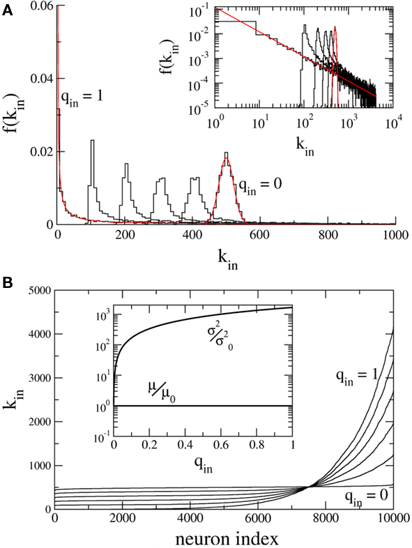
Figure 1. Hybrid degree distributions are generated by interpolating between a binomial and a power-law. (A) The histograms of in-degree from a network of 10,000 neurons in which the out-degree distribution was binomial. Here q_in = 0, 0.2, 0.4, 0.6, 0.8, 1.0. Inset: The same, but on a log–log scale. The analytical curves for the binomial and power-law distributions are shown in red. (B) In the same network as in (A), the neurons are ordered according to in-degree. Inset: As q_in is varied, the mean in-degree is fixed by construction but the variance increases monotonically. μ₀ and are the values of the mean and the variance for q_in = 0.

Integrate-and-Fire Model and Parameters

For q_in = q_out = 0, the I and EI networks are identical to those studied in Brunel and Hakim (1999) and Brunel (2000) respectively, with the sole exception that the in-degree in Brunel (2000) was a delta function and here it is Binomial for q_in = 0. This difference has no qualitative effect on the dynamics. The membrane potential of a neuron i is modeled as

with the reset condition V_i(t⁺) = V_reset whenever V_i(t⁻) ≥ θ. After reset, the voltage is fixed at the reset potential for a refractory period τ_rp = 2 ms. Postsynaptic currents (PSCs) are modeled as delta functions where J_ij is the strength of the connection from neuron j to neuron i, is the kth spike of neuron j, and D is a fixed delay. Connections are made according to the prescription described in the previous section for the hybrid degree distributions. In the EI network only the EE connections are made in this way. Other connectivities (II, EI, IE) are standard random networks with p = 0.1. If neuron j is excitatory (inhibitory) then, if a synapse is present, J_ij = J_E (J_I). External inputs are modeled as independent Poisson processes, each with rate ν_ext. PSCs are instantaneous with amplitude J_ext. For all neurons τ = 20 ms, V_reset = 10 ms and θ = 20 mV.

i. Inhibitory network: J_I = −0.1 mV, D = 2 ms, J_ext = 0.04 mV, v_ext = 30,000 Hz.

ii. Excitatory–inhibitory network: J_E = 0.1 mV, J_I = −0.45, D = 1.5 ms, J_ext = 0.12 mV, ν_ext = 8100 Hz.

Measures of Correlation

In several figures CC of synaptic inputs and of spikes are shown. The measures I used to generate these figures are given here.

Autocorrelation of the instantaneous firing rate

The spike train of a neuron i, s_i(t) was 1 if a spike was emitted in a time interval (t, t + Δt), and otherwise 0, where Δt was taken to be 1 ms. The instantaneous firing rate of the network where N is the total number of neurons in the network. The autocorrelation was

where the brackets denote a time average and the normalization is chosen so that the AC at zero-lag is equal to one.

Cross-correlations of synaptic inputs

In the network simulations, inputs consist of instantaneous jumps in the voltage of amplitude J_E (J_I) for excitatory (inhibitory) inputs. For each neuron i I define I_E,i(t) (I_I,i(t)) as the excitatory (inhibitory) input by summing the jumps in bins of 1 ms, i.e., t ∈ {0, 1, 2, 3, …} ms. Then the CC of the α ∈ {E, I} current in neuron i with the β ∈ {E, I} current in neuron j is written

where the brackets indicate a time average. The CC averaged over pairs is then In all simulations, CCs are calculated for n = 300 randomly chosen neurons.

Cross-correlation of spike-count

The spike train s_i(t) was convolved with a square kernel of duration T to yield the spike-count n_i(t). For the I network T = 10 ms while for the EI network T = 50 ms. The CC coefficient of the spike-count was then

Results

I performed simulations of large networks of sparsely connected spiking neurons with different in-degree and out-degree distributions. Randomly connected networks were generated with parameters q_α, α ∈ {in, out} which allowed for interpolation between Binomial degree distributions (q_α = 0) and Power-law degree distributions (q_α = 1) independently for the incoming and outgoing connections. For q_in = q_out = 0, the network was a standard random network which results when assuming a fixed probability of connection between any two neurons. I first studied the effect of degree distribution on fast oscillations in a network of inhibitory neurons. I subsequently studied slower oscillations in a network of excitatory and inhibitory neurons, which emerge due to an dynamic imbalance between excitation and inhibition. In both cases the focus was on the effect of the degree distribution on the transition between asynchronous and oscillatory behavior. This transition was most strongly modulated by the in-degree distribution and can be understood by analyzing a simple rate model. Finally, the out-degree distribution strongly affected the pairwise CC of synaptic currents in the network, but the effect on spiking correlations depended crucially on the dynamical state of the network as a whole.

A Network of Inhibitory Neurons

Dynamical states

The network consisted of 10,000 neurons driven by external, excitatory Poisson inputs and connected by inhibitory synapses modeled as a fixed delay followed by a jump in the postsynaptic voltage, see Section “Materials and Methods” for details. The mean in-degree and out-degree were fixed at 500. Parameter values were chosen such that fast oscillations were present in the network activity for q_in = q_out = 0. In this network, the frequency of oscillations is determined by the synaptic delay (Brunel and Hakim, 1999) while in more biophysically realistic networks the frequency is determined by both the synaptic kinetics, the membrane time constant, and the dynamics of spike generation (Brunel and Wang, 2003; Geisler et al., 2005). While coherent oscillations are observed in the instantaneous firing rate of the network activity, individual neurons fire irregularly at rates far below the oscillation frequency (Brunel and Hakim, 1999).

The fast oscillations in the network activity were suppressed by broadening the in-degree (increasing q_in) but were not strongly affected by broadening the out-degree (increasing q_out). This is illustrated in Figure 2 which shows rasters of the spiking activity of all inhibitory neurons for the standard random network (top), with broad in-degree (middle q_in = 0.6), and broad out-degree (bottom q_out = 0.6).

FIGURE 2

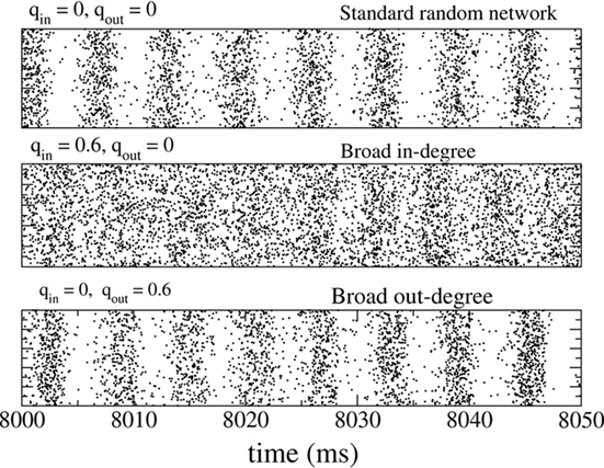
Figure 2. The spiking activity of all neurons in the standard random network (top), for broad in-degree (middle) and broad out-degree (bottom). Broadening the in-degree suppresses oscillations.

Figure 3 shows the amplitude of network oscillations and the mean firing rate in the network as a function of q_in and q_out. Oscillation amplitude is defined as the amplitude of the first side-peak in the autocorrelation function of the instantaneous firing rate, see Section “Materials and Methods.” As suggested by Figure 2, a transition from oscillations to asynchronous activity occurs as q_in increases, while varying q_out has little effect on the dynamical state of the network.

FIGURE 3

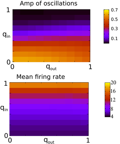
Figure 3. The presence of fast oscillations is strongly dependent on in-degree but not on out-degree. Top: The amplitude of the secondary peak in the AC of the instantaneous firing rate averaged over all neurons in the network during 10 s. Bottom: the firing rate in Hz averaged over all neurons and over 2 s. Both q_in and q_out were varied by increments of 0.1 from 0 to 1 for a total of 121 simulations.

A rate model

The effect of the in-degree can be captured in an extension of a rate model invoked to capture the generation of fast oscillations in inhibitory networks (Roxin et al., 2005). The model describes the temporal evolution of the mean activity level in the network and consists of a delay-differential equation. The equation cannot be formally derived from the original network model, but rather is a heuristic description of the network activity, meant to capture salient aspects of the dynamics, specifically transitions between asynchronous and oscillatory activity.

The equation is

where k is the in-degree index of a neuron, normalized so that k ∈ [0, 1]. It can be thought of as the index of a neuron in the network once all neurons have been ordered by increasing in-degree, as in Figure 1B. Therefore, r(k, t) represents the activity of a population of cells with in-degree index k at time t, I is an external current, D is a fixed temporal delay and The fact that the input to a neuron is dependent on its in-degree is modeled via the function where h(k) is a monotonically increasing function in k and q is meant to model the effect of q_in from the network simulations. Thus, J(k) is related to the inverse of the cumulative degree distribution as shown in Figure 1B. When q = 0, all neurons receive the same recurrent input, while increasing q results in neurons with higher index k receiving larger input. Importantly, h(k) is chosen so that which is equivalent to fixing the mean in-degree in the network.

The steady state meanfield solution is given by 〈r〉 = 〈R〉, where

The linear stability of the steady state solution depends only on the meanfield 〈R〉 and can be found by assuming a small perturbation of the steady state solution Eq. 9 of frequency ω. The critical frequency of the instability on the boundary between steady activity and oscillations is given by the equation ω =−tanωD, while the critical coupling on this line is determined by the condition

where

The stability of the steady state solution therefore depends on the gain of each neuron, weighted by the in-degree of that neuron and averaged over the entire network. The function ɸ(q) is an in-degree-dependent coefficient which modulates the gain of the network compared to the standard random network. For simplicity I will call it an effective gain. If q = 0 then all neurons have the same gain and ɸ = 1. If ɸ < 1 (ɸ > 1) then oscillations are suppressed (enhanced).

For simplicity I first consider the case of a threshold linear transfer function, Φ(I) = [I]₊, i.e., Φ(I) = I for I > 0 and is zero otherwise. I choose h(k) = 2k. See the Section “Appendix” for an analysis with more general function h(k). In this case, the steady state meanfield solution is

The mean activity increases as q increases beyond see the black line in Figure 4A (solid for dashed for ).

FIGURE 4

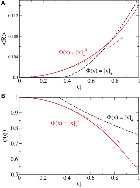
Figure 4. Broadening the in-degree distribution in the rate model Eq. 8 leads to increased mean activity and the suppression of fast oscillations. (A) The mean activity as a function of q for a linear-threshold transfer function (black) and a quadratic threshold transfer function (red). The dotted line is the asymptotic expression for small q for the quadratic case, Eq. 14. (B) The effective gain ɸ as a function of q for a linear-threshold transfer function (black) and a quadratic threshold transfer function (red). The dotted line is the asymptotic expression for small q for the quadratic case, Eq. 15. In (A,B) solid and dashed lines are for values of q for which the argument of the transfer function is always positive or is negative for some values of k respectively. Here J = 3 and I = 0.4,0.616 for the linear and quadratic cases respectively.

The effective gain function is

It can be seen upon inspection of Eq. 13 that ɸ(q) always decreases as the in-degree broadens, see Figure 4B. For the threshold linear function, once all neurons with receive inhibition sufficient to silence them, see the Section “Appendix” for details. Since the gain of these neurons is zero, and the gain of the remaining neurons is independent of k because of the linear transfer function, ɸ(q) necessarily decreases.

Figure 5 shows a phase diagram as a function of and q for oscillations in Eq. 8 with a threshold linear transfer function. To compare with network simulations we fix at a value for which oscillations spontaneously occur, e.g., circle in Figure 5, and increase q. This leads to a gradual reduction in oscillation amplitude until the steady state solution stabilizes, e.g., square in Figure 5. Space–time diagrams of the activity r(k, t) from the rate equation Eq. 8 are shown below the phase diagram. Below the space–time plots are representative raster plots from network simulations with q_in = 0.2 (left) and q_in = 0.8 (right) with the neurons ordered by increasing in-degree. Note the qualitative similarity.

FIGURE 5

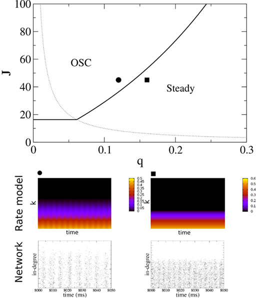
Figure 5. The phase diagram for an inhibitory network with hybrid in-degree distribution and threshold linear transfer function. The parameter q interpolates between the case of a standard random network and one with broad in-degree distribution. For the critical strength of inhibition (solid curve) increases with increasing q. Two sample color plots of the activity are shown below the diagram. The x-axis shows five units of time. Raster plots from network simulations with q_in = 0.2 (left) and q_out = 0.8 (right) are shown as a qualitative comparison.

The rate model Eq. 8 with a linear-threshold transfer function predicts that oscillations are suppressed as the in-degree broadens, in agreement with network simulations. How dependent is this result on the form of the transfer function? The steady state fI curve of integrate-and-fire neurons is not linear-threshold but rather it is concave-up for the range of firing rates in the simulations conducted here (Tuckwell, 1988). In fact, this is the case in general. For example, the transfer function of Hodgkin–Huxley conductance based model neurons as well as that of real cortical pyramidal neurons driven by noisy inputs is well fit by a power-law with power greater than one (Hansel and van Vreeswijk, 2002; Miller and Troyer, 2002). Therefore, it is important to know how the effective gain ɸ will change as a function of q given a concave-up transfer function. In fact, this can be understood intuitively. In the I network, for non-zero q, neurons with high in-degree receive more inhibition than those with low in-degree. Therefore, high in-degree neurons have lower firing rates and their gain is less. Since the gain of high in-degree neurons is weighted more than that of low in-degree neurons, the effective gain will decrease as q increases. Therefore, a concave-up transfer function will also lead to the suppression of oscillations for increasing q in the I network.

To quantify the above intuitive argument, if q ≪ 1 then one can obtain asymptotic formulas for the steady state solution and effective gain ɸ for arbitrary Φ and J(k), see Section “Appendix.” To take a simple example, if the transfer function is a rectified power-law, i.e., then, assuming x > 0 for all k, which is always true for small enough q

where R₀ is the steady state solution for q = 0, and Therefore, consistent with the intuitive argument made above, oscillations are suppressed for Φ concave up (α > 1) as long as J is large enough, since C₂/C₃ ∼ J. In fact, at the stability boundary J scales as 1/D for small delays and so is much larger than one. The functions 〈R〉 and ɸ are shown for the case α = 2 in Figures 4A,B. The solid and dashed lines are from the exact solution (dashed once the argument reaches zero for k = 1), while the dotted lines are from Eqs. 14 and 15.

Pairwise correlations

Pairwise spiking correlations in neuronal networks can arise from various sources including direct synaptic connections between neurons as well as shared input (Shadlen and Newsome, 1998; de la Rocha et al., 2007; Ostrojic et al., 2009). In the simulations performed here, the average probability of direct connection between any two neurons does not change as q_out is varied since the mean number of connections μ_out is fixed. However, the number of shared inputs is strongly influenced not only by the mean out-degree, but also by its variance . In fact, the expected fraction of shared inputs for any pair in the network can be calculated straightforwardly from the out-degree. If a neuron l has an out-degree k_l, then the probability that neurons i and j both receive a connection from l is just One can calculate the expected value of this quantity in the network by summing over all neurons and weighting by the out-degree of each neuron. This is equivalent to summing over all out-degrees, weighted by the out-degree distribution. This leads to (for N ≫ 1)

In the simulations conducted here, increasing q_out from 0 to 1, lead to approximately a fourfold increase in E_f. This increase in the fraction of common input may be expected to cause a concomitant increase in the correlation of input currents to pairs of neurons. However, the degree to which this increase translates into an increase in the correlation of pairwise spike-counts is strongly affected by both the filtering properties of the membrane potential, as well as the spiking mechanism of the model cells, which for integrate-and-fire neurons is just a reset. Here spike-count CCs are always very weak despite large current CCs. The reasons for this are discussed below.

Here, despite large CCs in the currents, the pairwise CC of the membrane potential is very weak. This is shown in Figure 6A, where the solid, dashed and dotted lines are the CCs of the inhibitory currents, the total current (inhibitory plus external drive) and the membrane potential respectively. It is clear that although the noise introduced by the external Poisson inputs reduces the CC of the input currents already by a factor of almost two, the CC of the membrane potential is an order of magnitude smaller. This very low correlation leads to small spike-count correlations. The distribution of the spike-count correlations at zero-lag in the network is shown in the left inset of Figure 6 (bin size of 10 ms), while the right inset indicates how the mean of this distribution changes as a function of the bin size used to count spikes. Why is the CC of the membrane potential so small? Some of the reduction in correlation is due to the low-pass filtering of the noisy oscillatory current. Specifically, while the noise amplitude is always reduced (by a factor of 1/2) by the low-pass filter, the effect on the oscillation amplitude depends on the value of the membrane time constant with respect to the oscillation frequency. For τ > 1/ω the oscillation amplitude is reduced, and for sufficiently long τ it is reduced much more than 1/2, see the Section “Appendix” for details. This results in reduced correlations since the unnormalized CC (which is proportional to the oscillation amplitude) is much less than the variance of the signal, which is proportional to the oscillation amplitude plus the noise amplitude. For the simulation used to make Figure 6 this filtering effect can be estimated to reduce the CC of the voltage about threefold compared to the current, see the Section “Appendix.” The remaining reduction in the CC must be attributable to the reset of the membrane potential after spiking. Since spiking is nearly uncorrelated on average between pairs, see the left inset of Figure 6, this results in large, nearly uncorrelated deflections of the membrane potential, driving down the CC of the voltage dramatically. The upshot is that spike-count correlations in networks of sparsely synchronized inhibitory neurons are very low. This is consistent with the dynamical regime in which neurons spike in a nearly Poisson way, at frequencies much lower than the frequency of the population oscillation.

FIGURE 6

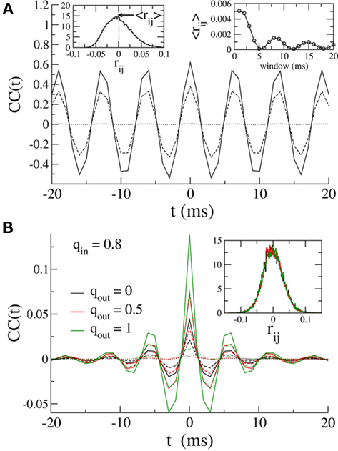
Figure 6. (A) Solid line: The average CC of the recurrent inhibitory current for q_in = q_out = 0. Dashed line: The average CC of the total current, including noisy external drive. Dotted line: The average CC of the voltage. Left inset: The distribution of pairwise spike-count correlations in 1 ms bins and smoothed with a 10-ms square window. The mean is given by the dotted line. Right inset: The mean pairwise spike-count correlation as a function of the window width used for smoothing. (B) The average CC for q_in = 0.8 and q_out = 0(black), 0.5 (red), and 1 (green). Increasing the out-degree increases the amplitude of the current CC (solid: inhibitory current, dashed: total current). However, membrane voltage CCs are much weaker, see dotted lines. Inset: The distribution of spike-count correlations is nearly unchanged.

Figure 6B shows how broadening the out-degree distribution affects pairwise correlations for q_in = 0.8, for which the network activity is only very weakly oscillatory. Increasing q_out from 0 (black) to 0.5 to 1 increases the amplitude of the CC of the recurrent inhibitory current significantly. However, filtering and reset effects of the model neurons once again reduce overall correlations (dashed line), and lead to spike-count correlations which are similar in all three cases, see inset.

Finally, Figure 7 shows the amplitude of the current CC at zero-lag and the mean spike-count CC as a function of q_in and q_out. When the network activity is weakly oscillatory or asynchronous, broadening the out-degree distribution increases the amplitude of the current CC as expected. This may account for the slight increase of oscillation amplitude for increasing q_out when q_in > 0.4 in Figure 3. However, this has little effect on the mean spike-count CC for the reasons described above.

FIGURE 7

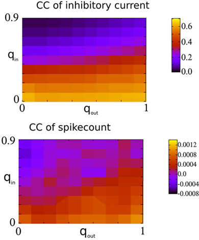
Figure 7. Spike-count CCs are only weakly dependent on the CCs of recurrent inhibitory currents in the I network. Top: The amplitude of the CC of the recurrent inhibitory current at zero-lag, see Figure 6 for an example. Bottom: The mean spike-count CC using a bin size of 1 ms and convolved with a square kernel of 10 ms duration.

A Network of Excitatory and Inhibitory Neurons

Dynamical states

The network consisted of 10,000 excitatory neurons and 2500 inhibitory neurons driven by external, excitatory Poisson inputs and connected by synapses modeled as a fixed delay followed by a jump in the postsynaptic voltage, see Section “Materials and Methods” for details. Only the degree distributions of the recurrent excitatory connections were varied (mean degree 500), while the other three connectivities were made by randomly connecting neurons with a fixed probability p = 0.1. The dynamical states of this network for q_in = q_out = 0 have been characterized numerically and analytically (Brunel, 2000) and it is known that slow oscillations can occur when inhibition is dominant and the external drive is not too strong. This is the case here. Nonetheless parameter values were chosen such that the network activity was asynchronous and at less than 1 Hz for q_in = q_out = 0, see Figure 8 (top). As for the inhibitory network studied previously, the spiking activity of individual neurons is highly irregular.

FIGURE 8

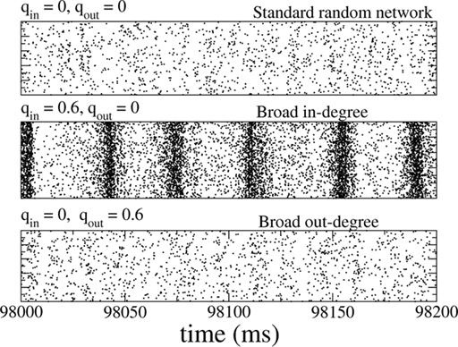
Figure 8. The spiking activity of all excitatory neurons in the standard random network (top), for broad in-degree (middle), and broad out-degree (bottom). Broadening the in-degree generates oscillations.

Slow (25 Hz) oscillations emerged as the in-degree was broadened, see Figure 8 (middle), while broadening the out-degree did not, in general, generate oscillations, see Figure 8 (bottom). The raster plots show the activity of all 10,000 excitatory neurons.

Figure 9 shows the amplitude of the first side-peak in the AC (top), and the firing rate in Hertz (bottom) averaged over all excitatory neurons. The presence of oscillations is clearly most strongly affected by changes in the in-degree, although there is some modulation of oscillation amplitude and firing rate by the out-degree.

FIGURE 9

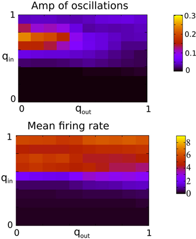
Figure 9. The presence of oscillations is strongly dependent on in-degree but not on out-degree. The amplitude of the oscillations is however significantly modulated by the out-degree. Top: The amplitude of the first side-peak in the AC of the instantaneous firing rate averaged over all excitatory neurons in the network during 100 s. Bottom: the firing rate in Hz averaged over all excitatory neurons and 2 s. Both q_in and q_out were varied by increments of 0.1 from 0 to 1 for a total of 121 simulations.

A rate model

As before, one can understand how the in-degree affects oscillations in the network by studying a rate model. The model now includes two coupled equations

where r_e(k, t) and r_i(t) represent the activity of neurons in the excitatory and inhibitory populations respectively, and τ is the ratio of the inhibitory to excitatory time constants. Here k ∈ [0, 1] represents the normalized index of a neuron in the excitatory population, once the neurons have been ordered by increasing in-degree, as in Figure 1B. The recurrent excitatory weights are written as where

I assume that the external input to the inhibitory population I_i is large enough that the total input is always greater than zero. Then the steady state meanfield activity of the excitatory population is

where , and The linear stability of this solution to oscillations can be studied by assuming small perturbations of frequency ω, see the Section “Appendix” for details. On the stability boundary

where and ɸ(0) = 1.

Again I look at the simple case of a threshold linear transfer function. Choosing h(k) = 2k yields for the steady state solution

the stability of which is determined by

By inspection, it is clear that ɸ(q) decreases for increasing q. Similar to the case of the purely inhibitory network, the reason ɸ decreases is that for neurons with receive insufficient input to be active. Their gain is now zero and that of the active neurons has not changed since the transfer function is linear. Thus for a linear-threshold transfer function oscillations are suppressed, in contradiction to what was observed in simulations of the EI network. This discrepancy can be explained by considering a concave-up transfer function Φ, which more closely resembles the fI curve of the integrate-and-fire neurons in the network simulations. Neurons with high in-degree in their recurrent excitatory connections fire at higher rates. Given a concave-up transfer function, the high in-degree neurons will therefore have a higher gain. Since they are weighted more than the low in-degree neurons, the effective gain is expected to increase, thereby enhancing oscillations. This is now consistent with the EI network simulations and is precisely the opposite of what was seen in the I network. Here again it is illustrative to look at the case q ≪ 1 for arbitrary Φ and J_ee(k), see Section “Appendix” for the full formulas. Assuming a power-law for the transfer function Φ(x) = x^α gives

where for simplicity. It is clear that if α ≥ 2 oscillations will always be enhanced. Therefore, although both the threshold linear and non-linear, concave-up functions lead to increasing firing rates as a function of q, see Figure 10A, the former will suppress oscillations while the latter enhances them, Figure 10B.

FIGURE 10

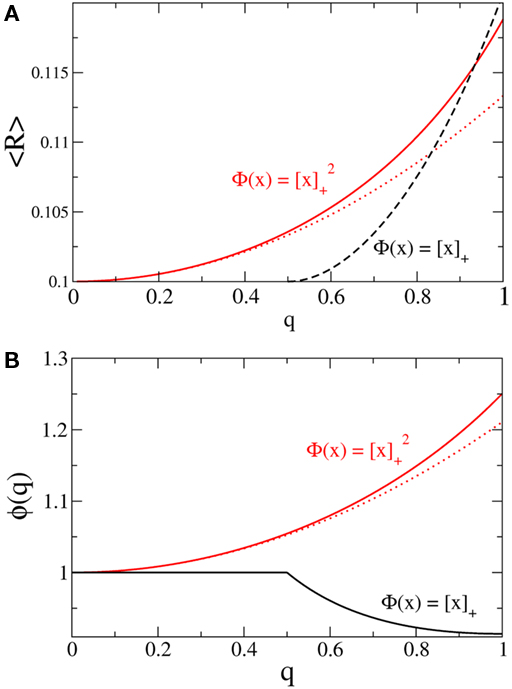
Figure 10. The effect of in-degree on the effective gain in an EI network depends crucially on the shape of the transfer function. (A) Both threshold linear and threshold quadratic transfer functions lead to increasing firing rate as q increases. (B) The threshold linear transfer function suppresses oscillations (decreasing ɸ) while the threshold quadratic transfer function enhances them (increasing ɸ). Parameters are for the linear and quadratic cases respectively. Black lines: threshold linear (dashed for q ≥ 1/J_ee). Red lines: threshold quadratic. Dotted lines: asymptotic formulas Eqs. 24 and 25.

Figure 11 shows the phase diagram for a threshold quadratic non-linearity as a function of and q, see the figure caption for parameters. Specifically, the transfer function is taken to be for x < 1 and for x > 1, which ensures that the activity will saturate once the instability sets in. However, the steady state value of x is less than one in simulations and hence the quadratic portion of the curve determines the stability. As predicted, the steady state becomes more susceptible to oscillations as q is increased. To compare with network simulations, we fix J_ee and increase q, causing the stable steady state solution, e.g., solid circle in phase diagram, to destabilize to oscillations, e.g., solid square in phase diagram. The resulting states are shown in the space–time plots below the phase diagram. Illustrative raster plots from network simulations with q_in = 0.4 and q_in = 0.6 are also shown in which the neurons are ordered by in-degree. Note the qualitative similarity.

FIGURE 11

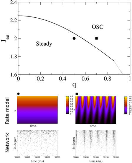
Figure 11. The phase diagram for the rate equations, Eq. 18 with hybrid in-degree distribution and threshold quadratic transfer function. The parameter q interpolates between the case of a standard random network and one with broad in-degree distribution. The dotted line indicates a rate instability, i.e., for ω = 0. Two sample color plots of the activity are shown below the diagram. The y-axis is k and the x-axis shows five units of time. Parameters are: J_ee = 2, J_ii = 0, I_e = 1, τ = 0.8. In the raster plots, only neurons 5000–10,000 are shown. The remaining neurons are essentially silent.

Pairwise correlations

In this network one would expect increasing the variance of the out-degree distribution to lead to an increase in the amplitude of CC in the recurrent excitatory input. This is indeed the case, as can be seen in Figure 12A, which shows the average CC between the excitatory component of the recurrent input in a pair of neurons. Here q_in = 0 and q_out = 0 (solid black) 0.2, 0.4, 0.6, 0.8 (dotted black) and 1 (red). The CC of the inhibitory current is unaffected by changes in the out-degree distribution of the recurrent excitatory connections as expected, see Figure 12B, while the CC between the excitatory component in one neuron and the inhibitory component in another is again strongly affected, see Figure 12C. The IE component of the CC is reflection symmetric about the origin to the EI component and is not shown. The pairwise CC of the total recurrent input, shown in Figure 12D (solid line) is unchanged as q_out increases, indicating that the increase in correlation amplitude of the EE component is balanced by the increase in the EI and IE components. Also shown is the CC of the total current including external inputs (dashed line) and the CC of the voltage (dotted lines). Thus pairwise correlations of the membrane voltage are weak and independent of out-degree. The inset shows the distributions of the pairwise spike-count correlations in a bin of 50 ms, and over 100 s of simulation time.

FIGURE 12

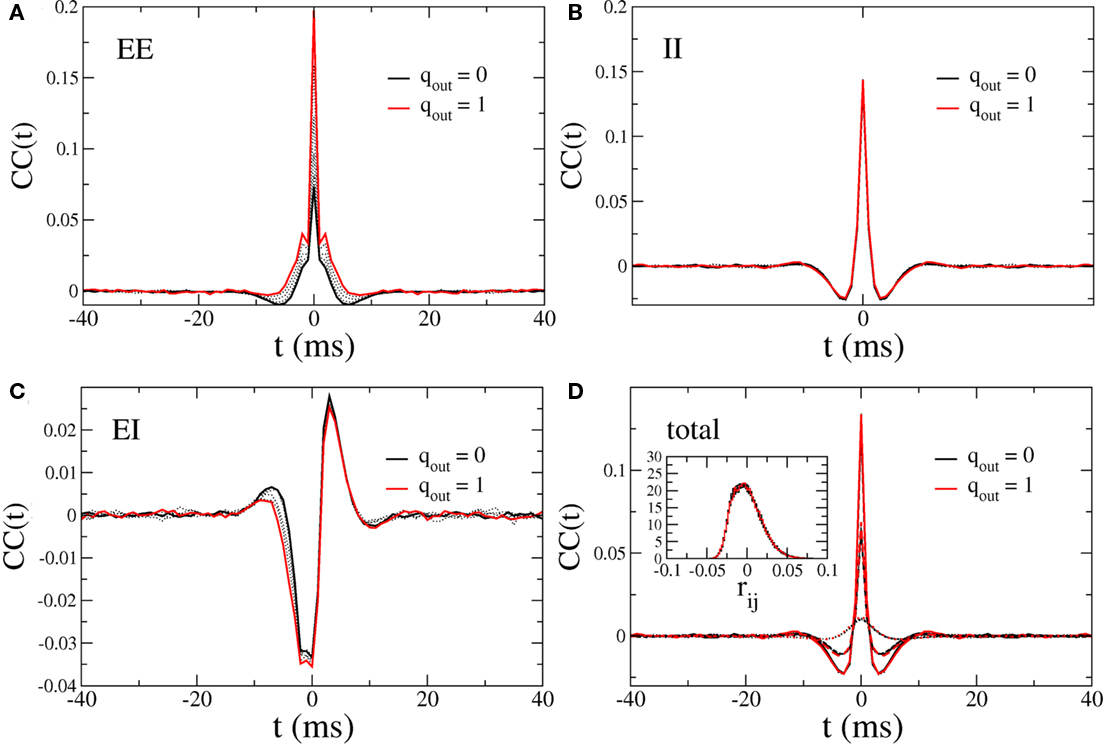
Figure 12. Cross-correlations (CC) of the various components of the synaptic inputs. (A) The pairwise correlation of the excitatory input. (B) The pairwise correlation of the inhibitory component. (C) The correlation of the excitatory component in one neuron with the inhibitory component in another, averaged over pairs. (D) The pairwise correlation of the total current. Solid line: CC of total recurrent input current. Dashed line: CC of total current including external input. Dotted line: CC of voltage. Inset: the distribution of pairwise spike-count correlations with a bin size of 1 ms. All curves are for q_out = 0 (solid black line), 0.2, 0.4, 0.6, 0.8 (dotted black curves), and 1 (solid red curve), and for q_in = 0.

Figure 13 shows the CC at zero-lag of the excitatory component of the current and the mean pairwise spike-count correlation as a function of q_in and q_out. It is clear that despite the strong dependence of the CC amplitude of the excitatory current on out-degree, the balancing described above renders the mean spike-count correlation essentially independent of out-degree and weak in the asynchronous regime. Mean spike-count correlations do, however, increase significantly in the presence of the 25-Hz oscillations, i.e., as q_in increases beyond a critical value, see the top panel in Figure 9. In this regime, the mean spike-count correlation is significantly affected by changes in the out-degree distribution. This is likely due to the disruption of the dynamical balance which is responsible for the cancelation of subthreshold correlations in the asynchronous regime (Renart et al., 2010).

FIGURE 13

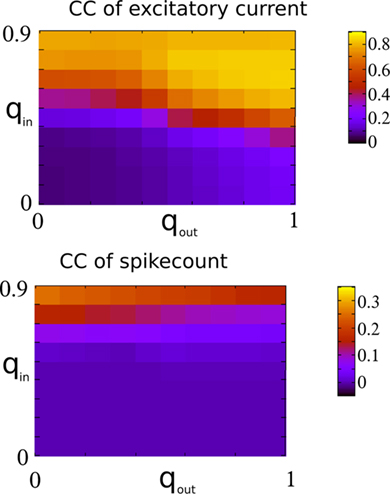
Figure 13. Top: The CC at zero-lag of the recurrent excitatory input in the excitatory–inhibitory network. Bottom: The mean pairwise spike-count correlation in the excitatory–inhibitory network. CC were averaged over 100 s of simulation time.

In fact, broadening the out-degree distribution can even lead to qualitative changes in the dynamical state of the network, as long as the system is poised near a bifurcation. This is shown in Figure 14 for q_in = 0.4 (right below the bifurcation to oscillations), which for q_out = 0 exhibits asynchronous activity (top), while increasing q_out generates synchronous, aperiodic population spikes (middle and bottom).

FIGURE 14

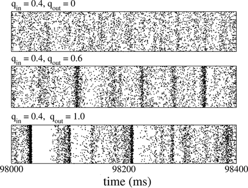
Figure 14. Changing the out-degree can qualitatively affect the dynamical state of the network near a bifurcation. Here, the network is poised just below the instability to 25 Hz oscillations (q_in). When q_out = 0 (top) the activity is asynchronous. Broadening the out-degree leads to synchronous population bursts (q_out = 0.6, 1 middle and bottom).

Discussion

I have conducted numerical simulations of two canonical networks as a function of the in-degree and out-degree distributions of the network connectivity. For both the purely inhibitory (I), as well as the EI networks, it was the in-degree which most strongly affected the global, dynamical state of the network. In both cases, increasing the variance of the in-degree drove a transition in the dynamical state: in the I network oscillations were abolished while in the EI network, oscillations were generated when the E-to-E in-degree was broadened. The analysis of a simple rate model, suggests that these transitions can be understood as the effect of in-degree on the effective input–output gain of the network. Specifically, in a standard random network with identical neurons, the gain of the network in the spontaneous state can be expressed as the slope of the non-linear transfer function which converts the total input to neurons into an output, e.g., a firing rate. This is the approximation made in a standard, scalar rate equation. A high gain makes the network more susceptible to instabilities, e.g., oscillations. In the case of a network with a broad in-degree distribution, each neuron receives a different level of input, and the effective gain is now the gain of each neuron, averaged over neurons and weighted by the in-degree. In this way the stability of the spontaneous state may depend crucially on the shape of the transfer function. The transfer function for integrate-and-fire neurons in the fluctuation-driven regime is concave-up. For this type of transfer function, the simple rate equation predicts that oscillations will be suppressed in the I network and enhanced in the EI network, in agreement with the network simulations. It has been shown that the single-cell fI curve of cortical neurons operating in the fluctuation-driven regime is well approximated by a power-law with power greater than one (Hansel and van Vreeswijk, 2002; Miller and Troyer, 2002), indicating that the above argument should also be valid for real cortical networks. Furthermore, the heterogeneity in gain across neurons need not be due specifically to differences in in-degree for the above argument to hold. Thus the rate equation studied here should be valid given other sources of heterogeneity in gain, e.g., in the strength of recurrent synapses. Although I have focused here on the in-degree distribution of the E-to-E connections in the EI network, this work suggests that the effect of in-degree in the other three types of connections (E-to-I, I-to-I, and I-to-E) can be captured just as easily in the firing rate model. A complete analysis in this sense goes beyond the scope of this paper, which sought merely to establish the validity of the firing rate model for in-degree.

The out-degree distribution determines the amount of common, recurrent input to pairs of neurons, and as such may be expected to affect pairwise spiking correlations. Yet predicting spike correlations based on knowledge of input correlations has proven a non-trivial task and can depend crucially on firing rate, external noise amplitude, and the global dynamical state of the network to name a few factors (de la Rocha et al., 2007; Ostrojic et al., 2009; Hertz, 2010; Renart et al., 2010). Here, pairwise spike-count correlations in the I network were always very low despite the relatively high CC of input currents. This is attributable to the very low CC of the membrane voltage which, in turn, is due to the combined effects of low-pass filtering a noisy, fast oscillatory input and large, uncorrelated (across neurons) fluctuations due to the spike reset. In the case of the EI network, the drastic decrease in CCs from currents to membrane voltage to spike-count was studied previously in the same network with standard random connectivity (Kriener et al., 2008; Tetzlaff et al., 2008), and has been observed in networks with synaptic input modeled as conductances (Kumar et al., 2008; Hertz, 2010). Furthermore, low spike-count correlations appear to be a generic and robust feature of spiking networks in the balanced state (Renart et al., 2010). In the simulations conducted here, increasing the fraction of common input had a significant effect on the amplitude of excitatory current CCs. However, in the asynchronous regime, fluctuations in excitatory currents were followed by compensatory fluctuations in inhibitory currents with very small delay, as evidenced by the CCs shown in Figure 12C and resulting in narrow CCs of the total current, see Figure 12D. This cancelation left the CCs of the spike-count essentially unaffected by changes in the out-degree. On the other hand, once the network is no longer in the asynchronous regime, the fraction of common input has a significant effect on spike-count correlations as well as the global dynamical state of the network. In this case changes in the out-degree can even drive transitions to qualitatively new dynamical regimes, such as the aperiodic population bursts seen in Figure 14. These dynamics have not been characterized in detail here.

The in-degree and out-degree distributions alone may not be sufficient to characterize the connectivity in real neuronal networks. As an example, while broad degree distributions lead to an over-representation of triplet motifs compared to the standard random network, e.g., see Figure 11 in (Roxin et al., 2008), the probability of bidirectional connections is independent of degree. Therefore, to generate a network with connectivity motifs similar to those found in slices of rat visual cortex (Song et al., 2005) requires at least one additional parameter. Furthermore, correlations between in-degree and out-degree, which were not considered in this work, may have a significant impact on network dynamics. For example, in networks of recurrently coupled oscillators, increasing the covariance between the in-degree and out-degree has been shown to increase synchronization (LaMar and Smith, 2010; Zhao et al., submitted). Introducing positive correlations between in-degree and out-degree in the E-to-E connectivity in an EI network, for example, would mean that common excitatory inputs to pairs would also tend to be those with the highest firing rate. Allowing for such correlations would not be expected to significantly alter the dynamics in the balanced, asynchronous regime of the EI network due to the rapid dynamical cancelation of currents. However, it is likely that the stochastic population bursts observed near the onset to oscillations for broad out-degree distributions would be enhanced, see Figure 14.

How should one proceed in investigating the role of connectivity on network dynamics? As mentioned in the previous paragraph, there are other statistical measures of network connectivity which allow one to characterize network topology and conduct parametric analyses, e.g., motifs. No one measure is more principled than another and they are not, in general, independent. Parametric studies, such as this one, can shed light on the role of certain statistical features of network topology in shaping dynamics. Specifically, for networks of sparsely coupled spiking neurons, the width of the in-degree strongly affects the global dynamical state, while the width of the out-degree affects pairwise correlations in the synaptic currents. An alternative and more ambitious approach would allow synaptic connections to evolve according to appropriate plasticity rules. In this way, the network topology would be shaped by stimulus-driven inputs and could then be related to the functionality of the network itself. Additional constraints, such as minimizing wiring length for fixed functionality, may lead to topologies which more closely resemble those measured in the brain (Chklovskii, 2004). A complementary future goal of such computational work should be to collaborate with experimentalists in defining aspects of network connectivity which can be reasonably measured with current methods and which also may play a key role in neuronal dynamics.

Conflict of Interest Statement

The author declares that the research was conducted in the absence of any commercial or financial relationships that could be construed as a potential conflict of interest.

Acknowledgments

I thank Duane Nykamp and Jaime de la Rocha for very useful discussions. I thank Rita Almeida, Jaime de la Rocha, Anders Ledberg, Duane Nykamp, and Klaus Wimmer for a careful reading of the manuscript. I would like to thank the Gatsby Foundation, the Kavli Foundation and the Sloan–Swartz Foundation for their support. Alex Roxin was a recipient of a fellowship from IDIBAPS Post-Doctoral Programme that was cofunded by the EC under the BIOTRACK project (contract number PCOFUND-GA-2008-229673). This work was funded by the Spanish Ministry of Science and Innovation (ref. BFU2009-09537), and the European Regional Development Fund.

References

Amit, D. J., and Brunel, N. (1997a). Dynamics of a recurrent network of spiking neurons before and following learning. Network 8, 373–404.

CrossRef Full Text

Amit, D. J., and Brunel, N. (1997b). Model of global spontaneous activity and local structured activity during delay periods in the cerebral cortex. Cereb. Cortex 7, 237–252.

CrossRef Full Text

Barbieri, F., and Brunel, N. (2007). Irregular persistent activity induced by synaptic excitatory feedback. Front. Comput. Neurosci. 1:5. doi: 10.3389/neuro.10/005.2007

Pubmed Abstract | Pubmed Full Text | CrossRef Full Text

Brunel, N. (2000). Dynamics of sparsely connected networks of excitatory and inhibitory spiking neurons. J. Comput. Neurosci. 8, 183–208.

Pubmed Abstract | Pubmed Full Text

Brunel, N., and Hakim, V. (1999). Fast global oscillations in networks of integrate-and-fire neurons with low firing rates. Neural Comput. 11, 1621–1671.

Pubmed Abstract | Pubmed Full Text | CrossRef Full Text

Brunel, N., and Hakim, V. (2008). Sparsely synchronized neuronal oscillations. Chaos 18, 015113.

Pubmed Abstract | Pubmed Full Text

Brunel, N., and Wang, X.-J. (2003). What determines the frequency of fast network oscillations with irregular neural discharges? J. Neurophysiol. 90, 415–430.

Pubmed Abstract | Pubmed Full Text | CrossRef Full Text

Chklovskii, D. B. (2004). Synaptic connectivity and neuronal morphology: two side of the same coin. Neuron 43, 609–617.

Pubmed Abstract | Pubmed Full Text

de la Rocha, J., Doiron, B., Shea-Brown, E., Josić, K., and Reyes, A. (2007). Correlation between neural spike trains increases with firing rate. Nature 448, 802–806.

Pubmed Abstract | Pubmed Full Text | CrossRef Full Text

de Solages, C., Shapiro, G., Brunel, N., Hakim, V., Isope, P., Buisseret, P., Rousseau, C., Barbour, B., and Léna, C. (2008). High frequency organization and synchrony of activity in the Purkinje cell layer of the cerebellum. Neuron 58, 775–788.

Pubmed Abstract | Pubmed Full Text | CrossRef Full Text

Ecker, A. S., Berens, P., Keliris, G. A., Bethge, M., Logothetis, N. K., and Tolias, A. S. (2010). Decorrelated neuronal firing in cortical microcircuits. Science 327, 584.

Pubmed Abstract | Pubmed Full Text

Geisler, C., Brunel, N., and Wang, X.-J. (2005). The contribution of intrinsic membrane dynamics to fast network oscillations with irregular neuronal discharges. J. Neurophysiol. 94, 4344–4361.

Pubmed Abstract | Pubmed Full Text | CrossRef Full Text

Hansel, D., and van Vreeswijk, C. (2002). How noise contributes to contrast invariance of orientation tuning in cat visual cortex. J. Neurosci. 22, 5118–5128.

Pubmed Abstract | Pubmed Full Text

Hertz, J. (2010). Cross-correlations in high-conductance states of a model cortical network. Neural Comput. 22, 427–447.

Pubmed Abstract | Pubmed Full Text | CrossRef Full Text

Holmgren, C., Harkany, T., Svennenfors, B., and Zilberter, Y. (2003). Pyramidal cell communication within local networks in layer 2/3 of rat neocortex. J. Physiol. 551, 139–153.

Pubmed Abstract | Pubmed Full Text | CrossRef Full Text

Kriener, B., Tetzlaff, T., Aertsen, A., Diesmann, M., and Rotter, S. (2008). Correlations and population dynamica in cortical networks. Neural Comput. 20, 2185–2226.

Pubmed Abstract | Pubmed Full Text | CrossRef Full Text

Kumar, A., Schrader, S., Aertsen, A., and Rotter, S. (2008). The high-conductance state of cortical networks. Neural Comput. 20, 1–43.

Pubmed Abstract | Pubmed Full Text | CrossRef Full Text

LaMar, M. D., and Smith, G. D. (2010). Effect of node-degree correlation on synchronization of identical pulse-coupled oscillators. Phys. Rev. E 81, 046206.

Mazzoni, A., Panzeri, S., Logothetis, N. K., and Brunel, N. (2008). Encoding of naturalistic stimuli by local field potential spectra in networks of excitatory and inhibitory neurons. PLoS Comput. Biol. 4, e1000239. doi: 10.1371/journal.pcbi.1000239

Pubmed Abstract | Pubmed Full Text | CrossRef Full Text

Miller, E. K., and Troyer, T. W. (2002). Neural noise can explain expansive, power-law nonlinearities in neural response functions. J. Neurophysiol. 87, 653–659.

Pubmed Abstract | Pubmed Full Text

Mishchenko, Y., Hu, T., Spacek, J., Mendenhall, J., Harris, K. M., and Chklovskii, D. B. (2010). Ultrastructural analysis of hippocampal neuropil from the connectomics perspective. Neuron 67, 1009–1020.

Pubmed Abstract | Pubmed Full Text | CrossRef Full Text

Newman, M. E. J. (2003). The structure and function of complex networks. SIAM Rev. 45, 167.

Newman, M. E. J., Strogatz, S., and Watts, D. J. (2001). Random graphs with arbitrary degree distributions and their applications. Phys. Rev. E 64, 026118.

Ostrojic, S., Brunel, N., and Hakim, V. (2009). How connectivity, background activity and synaptic properties shape the cross-correlation between spike trains. J. Neurosci. 29, 10234–10253.

Pubmed Abstract | Pubmed Full Text | CrossRef Full Text

Renart, A., Rocha, J., Bartho, P., Hollender, L., Parge, N., Reyes, A., and Harris, K. (2010). The asynchronous state in cortical circuits. Science 327, 587–590.

Pubmed Abstract | Pubmed Full Text | CrossRef Full Text

Roxin, A., Brunel, N., and Hansel, D. (2005). Role of delays in shaping spatiotemporal dynamics of neuronal activity in large networks. Phys. Rev. Lett. 94, 238103.

Pubmed Abstract | Pubmed Full Text

Roxin, A., Hakim, V., and Brunel, N. (2008). The statistics of repeating patterns of cortical activity can be reproduced by a model network of stochastic binary neurons. J. Neurosci. 28, 10734–10745.

Pubmed Abstract | Pubmed Full Text | CrossRef Full Text

Shadlen, M. N., and Newsome, W. T. (1998). The variable discharge of cortical neurons: implications for connectivity, computation, and information coding. J. Neurosci. 18, 3870–3896.

Pubmed Abstract | Pubmed Full Text

Shephard, G. M. G., Stepanyants, A., Bureau, I., Chklovskii, D., and Svoboda, K. (2005). Geometric and functional organization of cortical circuits. Nat. Neurosci. 8, 782–790.

Pubmed Abstract | Pubmed Full Text

Song, S., Sjöström, P. J., Reigl, M., Nelson, S., and Chklovski, D. B. (2005). Highly nonrandom features of synaptic connectivity in local cortical circuits. PLoS Biol. 3, 507–519. doi: 10.1371/journal.pbio.0030068

CrossRef Full Text

Tetzlaff, T., Rotter, S., Stark, E., Abeles, M., Aertsen, A., and Diesmann, M. (2008). Dependence of neuronal correlations on filter characteristics and marginal spike train statistics. Neural Comput. 20, 2133–2184.

Pubmed Abstract | Pubmed Full Text | CrossRef Full Text

Tuckwell, H. C. (1988). Introduction to Theoretical Neurobiology. Cambridge: Cambridge University Press.

van Vreeswijk, C., and Sompolinsky, H. (1996). Chaos in neuronal networks with balanced excitatory and inhibitory activity. Science 274, 1724–1726.

Pubmed Abstract | Pubmed Full Text | CrossRef Full Text

van Vreeswijk, C., and Sompolinsky, H. (1998). Chaotic balanced state in a model of cortical circuits. Neural Comput. 10, 1321–1371.

Pubmed Abstract | Pubmed Full Text | CrossRef Full Text