Information loss associated with imperfect observation and mismatched decoding

Introduction

Neurons in early sensory areas represent the information of various stimuli from the external world by their noisy activities. The noise inherent in neural activities needs to be properly handled by the nervous system for the information to be accurately processed. One simple but powerful means for coping with the neural noise is population coding. Neurophysiological experiments have shown that many neurons with different selectivities respond to particular stimuli. These findings suggest that the nervous system represents information through population activities, which would be helpful for accurate information processing. This coding scheme for stimulus information is known as population coding.

An important feature of population coding is that the activity of neurons is correlated (Gray et al., 1989; Gawne and Richmond, 1993; Zohary et al., 1994; Meister et al., 1995; Lee et al., 1998; Ishikane et al., 2005; Averbeck et al., 2006; Ohiorhenuan et al., 2010; but see Ecker et al., 2010). A crucial question is how much information the nervous system can extract from correlated population activities. In general, it is difficult for the nervous system to maximally extract information when its activities are correlated because two conditions must be satisfied. First, downstream neurons must perfectly observe the responses of the upstream neurons (perfect observation of neural responses). Second, downstream neurons must optimally decode the information from the observed neural responses (optimal decoding of stimulus). In other words, if either the observation or the decoding is imperfect or non-optimal, which are both likely situations in the nervous system, stimuli information is inevitably degraded. In this work, we discuss the amount of information loss associated with imperfect observation and non-optimal decoding.

With regard to non-optimal decoding, several researchers including the authors of this paper have investigated how much information would be lost if neural correlation is ignored in decoding (Nirenberg et al., 2001; Wu et al., 2001; Golledge et al., 2003; Averbeck and Lee, 2006; Oizumi et al., 2010). This type of decoding is called mismatched decoding (Merhav et al., 1994; Oizumi et al., 2010) because the decoding does not match the actual neural activities, i.e., the actual neural activities are correlated but the correlations are ignored in decoding. With regard to imperfect observation, this work is the first to address this issue. As an example of imperfect observation, we specifically consider the situation that the activity of neurons is not simultaneously observed by downstream neurons (Figure 1). This is related to whether the coincidence detector plays an important role in information processing in the brain (Abeles, 1982; König et al., 1996). If a large proportion of the total information is lost when the responses of neurons are not simultaneously observed, coincidence detection would be necessary for accurate information processing.

FIGURE 1

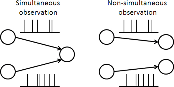
Figure 1. Schematic of simultaneous and non-simultaneous observation of neural responses.

The framework of mismatched decoding was introduced to quantify the importance of correlated activity because this importance could be quantified by the amount of information loss when neural correlation is ignored in decoding (Nirenberg et al., 2001; Wu et al., 2001; Nirenberg and Latham, 2003). Similarly, the importance of correlated activity could be also measured using the amount of information loss due to non-simultaneous observation. We therefore obtain two different measures for the importance of correlated activity by introducing the concepts of imperfect observation and mismatched decoding. We aim to clarify the relationship between the measures and provide a simple guide on how to use them.

Combining the concepts of imperfect observation and mismatched decoding produces four types of situations where stimulus is inferred: (1) observation is perfect and decoding is optimal; (2) decoding is optimal but observation is imperfect; (3) observation is perfect but decoding is mismatched; and (4) observation is imperfect and decoding is mismatched. We discuss the inferences in these four types of situations from the viewpoint of information geometry (Amari and Nagaoka, 2000) and then clarify their relationships. We also specifically compute the amount of information obtained through these four inference types for neural responses described by the Gaussian model and by a binary probabilistic model.

This paper is organized as follows. First, we introduce the concept of an exponential family and two probability distributions that belong to the exponential family, i.e., the Gaussian distribution and the binary probabilistic model, which have both been intensively investigated as representative models of neural responses (Abbott and Dayan, 1999; Amari, 2001; Nakahara and Amari, 2002). Second, we provide information geometric interpretation of the four types of inference mentioned above and describe how to evaluate the information in each of the four types by using the Fisher information. Third, we compute the amount of information in each of the four types of inference in the Gaussian model and explain the relationship between the inference with imperfect observation and that with mismatched decoding. Fourth, we also compute the amount of information obtained by the four types of inference in simple binary probabilistic models. Finally, we summarize the results and discuss how to use the two measures introduced in this study for quantifying the importance of neural correlation and mention some of the future directions of this work.

Exponential Family of Probability Distributions

Let us denote the conditional probability distribution for a neural response r = (r₁, r₂,…,r_N) over a population of N neurons being evoked by a stimulus s as p(r; s), where s is a continuous variable. We assume that p(r; s) belongs to the exponential family. Probability distributions that belong to an exponential family can be written as

where R_I(r) is a function of neural responses r, θ_I(s) is a function of stimulus s, and a normalization constant ψ(s) is also a function of stimulus s. θ_I(s) is called the natural parameter of the exponential family. Two examples of probability distributions are investigated in this paper.

Example 1. Gaussian Distribution

The number of spikes emitted by a neuron over a fixed time period (time-averaged rate) or the total number of spikes emitted by a population of neurons (population-averaged rate), which is denoted by r, may be described by the Gaussian distribution

where N is the number of neurons, f(s) is the average number of spikes, and C(s) is the covariance matrix. If we rewrite Eq. 2 as follows, we can see that the Gaussian distribution belongs to the exponential family

In this case,

Example 2. Log-linear Model of Binary Neural Response

When we analyze neural responses within a short time period (∼1–10 ms, typically), the neural responses are considered stochastic binary variables: r_i = 1 when the ith neuron fires within the time bin, and r_i = 0 when it does not. The joint distributions of N random binary variables can be generally written in the following form (Amari, 2001; Nakahara and Amari, 2002):

where the normalization constant ψ(s) is given by

This probability distribution is clearly in the exponential family form. In this case,

Recent investigations have shown that the observed statistics of neural responses can be sufficiently captured by this type of probabilistic model, which contains up to second-order correlation terms (Schneidman et al., 2006; Shlens et al., 2006; Tang et al., 2008), although the importance of higher-order correlations has also been discussed (Amari et al., 2003; Montani et al., 2009; Ohiorhenuan et al., 2010). For simplicity, we consider only the second-order correlations and ignore higher-order correlations in this work, i.e.,

Inference of Stimulus and Fisher Information

We consider the inference problem of how accurately the stimulus value s can be estimated when the stochastic neural response r is given. We assume that neural response r is observed many times. The neural response at the tth trial is denoted by r(t) and the number of trials by T. If each neural response is independent and identically distributed, the probability distribution for T observations of neural responses is given by

where are sufficient statistics for the probability distribution and are given by

We evaluate the accuracy of the estimate by using the Fisher information,

where l_s = log p_T(r^T; s) and denotes the expectation with respect to the distribution p_T(r^T; s). Through the Cramér–Rao bound, the Fisher information bounds the average squared decoding error for an unbiased estimate as follows:

where s is the true stimulus value and is the estimate. Since the Fisher information is the lower bound of the mean square error, behavior of the mean square error and the Fisher information could be different in general (Brunel and Nadal, 1998; Yaeli and Meir, 2010). However, the maximum likelihood estimator, which chooses s for an estimate that maximizes likelihood function p_T(r^T; s), achieves the Cramér–Rao bound (Eq. 19) as T → ∞. A Bayesian estimator, which is generally a biased estimator, can also achieve the Cramér–Rao bound as T → ∞ because it becomes equivalent to the maximum likelihood estimator as T → ∞.

We compute the Fisher information with respect to stimulus s from the Fisher information matrix with respect to the natural parameters,

where l_θ = p_T(r^T; θ), and ∂_I = ∂/∂θ_I. From the definition of the Fisher information matrix with respect to the natural parameters (Eqs. 20 and 21), the natural parameters are given by

where

By using g_IJ(θ), the Fisher information with respect to the stimulus s can be written as

The Fisher information g(s) described above determines the accuracy of the estimate of s under two conditions: (1) all sufficient statistics are available, and (2) the likelihood function p(r; s) is exactly known. Regarding the first condition, downstream neurons may not be able to simultaneously access the responses of all upstream neurons. This imperfect observation of neural responses by downstream neurons leads to loss of information. Similarly, regarding the second condition, downstream neurons are unlikely to completely know the likelihood function p(r; s). Downstream neurons are more likely to only partially know p(r; s) and to decode the stimulus based on a decoding model q(r; s), which is not equal to p(r; s) but partially matches p(r; s) (Nirenberg et al., 2001; Wu et al., 2001; Oizumi et al., 2010). This mismatched decoding of stimuli by downstream neurons also results in loss of information. These two types of information loss are evaluated next.

Information Loss Caused by Imperfect Observation of Neural Responses

In this work, we specifically consider the situation that second-order sufficient statistics are not accessible to downstream neurons and only first-order sufficient statistics are available to them. This is related to whether coincidence detector neurons are needed to accurately estimate the stimulus. To evaluate the loss of information associated with loss of data, we first marginalize the joint probability distribution over

When only is observed, the Fisher information with respect to stimulus s is given by

The information loss associated with loss of is

Information Loss Caused by Mismatched Decoding of Stimulus

We evaluate the loss of information when downstream neurons infer the stimulus parameter s based on not the correct probability distribution p(r; s) but a mismatched probability distribution q(r; s). We assume that q(r; s) also belongs to the exponential family and that the maximum likelihood estimation based on q(r; s) is consistent, i.e.,

where E_p denotes the expectation with respect to p(r; s) and l_q(r; s) = log q(r; s). We evaluate the squared decoding error of the maximum likelihood estimation with the mismatched likelihood function q(r; s) based on T observations of neural responses, r^T. The estimate is given by

By differentiating l_qT(r^T; s) with respect to s at we obtain the quasi-likelihood estimating equation

When the left-hand side terms of Eq. 32 are expanded at the true value of stimulus parameter s,

According to the central limit theorem, the first term on the right-hand side of Eq. 33 converges to a Gaussian distribution with mean 0 and variance TE_p[(dl_q(r; s)/ds)²] as T → ∞. From the weak law of large numbers, the coefficient of the second term on the right-hand side of Eq. 33 becomes

Taken together, we have

If we regard the inverse of the squared decoding error as the Fisher information, the Fisher information for mismatched decoding model q(r; s) is

Note that when q(r; s) = p(r; s), g*(s) = g(s).

Information Geometric Interpretations

We discuss the inference of stimulus when neural responses are only partially observed and that when a mismatched probability distribution is used for decoding, from the information geometric viewpoint (Amari and Nagaoka, 2000). We consider the following four types of inference.

Inference 1 (Perfect observation and matched decoding) The complete data are available and the true probability distribution p(r; s) is used for decoding.

Inference 2 (Imperfect observation) The true probability distribution p(r; s) is used for decoding but only partial data are available.

Inference 3 (Mismatched decoding) The complete data are available but a mismatched probability distribution q(r; s) is used for decoding.

Inference 4 (Imperfect observation and mismatched decoding) A mismatched probability distribution q(r; s) is used for decoding and only partial data are available.

We assumed that both the true probability distribution p(r; s) and mismatched probability distributions q(r; s) belong to the exponential family of probability distributions S given in Eq. 1. S is specified by n-dimensional natural parameters θ = (θ_1, θ_{2, …,} θ_n). If we take θ as a coordinate system introduced in set S of probability distributions, we can regard S as an n-dimensional manifold (space). A point in S represents a specific probability distribution determined by the parameters θ. The true statistical model p(r; s) denoted by M and the mismatched statistical model q(r; s) denoted by M*, both of which are parameterized by a single variable s, are considered as curves in the manifold S, i.e., one-dimensional submanifolds having a coordinate s.

Inference 1 First, we describe Inference 1 from the viewpoint of information geometry (Amari, 1982; Amari and Nagaoka, 2000). Let us denote the observed data by can be considered as a point in S, which we call the observed point. The observed point is distributed near the point s that represents the true probability distribution when stimulus s is presented, p(r; s). The deviation of from the point specified by the true stimulus parameter s can be decomposed into the deviation in the parallel direction to M and the deviation in the orthogonal direction to M. The maximum likelihood estimation corresponds to the minimizer of the Kullback–Leibler divergence between the distribution corresponding to the observed point (which is not in M in general) and distributions in M,

where is the maximum likelihood estimator. The geometric interpretation of the maximum likelihood estimation is the orthogonal projection to M from (Figure 2). The orthogonal projection completely eliminates the deviation of from s in the orthogonal direction to M but the deviation in the parallel direction to M remains. This remaining deviation corresponds to the Fisher information of M (Eq. 18). If we use other estimators that are not orthogonal projections to M (e.g., the moment estimator), the decoding error necessarily becomes larger than the orthogonal projection.

FIGURE 2

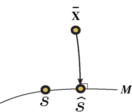
Figure 2. Information geometric picture of Inference 1 (perfect observation and matched decoding).

Inference 2 In the Inference 2 case (Amari, 1995), only is observed. Let us define a submanifold D, which is formed by the set of observed points, where is fixed at the observed value but unobserved takes arbitrary values. Submanifold D is called the data submanifold. The maximum likelihood estimation based on partial observed data corresponds to searching for the pair of points and that minimizes the Kullback–Leibler divergence between D and M (Figure 3), i.e.,

FIGURE 3

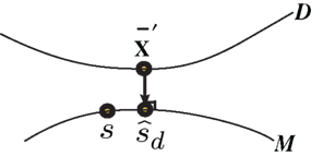
Figure 3. Information geometric picture of Inference 2 (imperfect observation).

The estimated value of s is expressed as

For a given candidate point in D, the point in M that minimizes the Kullback–Leibler divergence is given by the orthogonal projection of to M.

Inference 3 For Inference 3 (Figure 4), we assumed that the maximum likelihood estimation based on a mismatched model q(r; s) is unbiased (Eq. 29). This condition corresponds to the case where the point p(r; s) in M and the point q(r; s) in M*, which both represent a given stimulus parameter s, are the mutually nearest points in S in terms of the Kullback–Leibler divergence, i.e.,

FIGURE 4

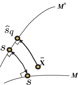
Figure 4. Information geometric picture of Inference 3 (mismatched decoding).

If we differentiate Eq. 40 with respect to s′, we obtain Eq. 29. Similar to in Inference 1, the maximum likelihood estimation based on a mismatched model M* corresponds to the minimization of the Kullback–Leibler divergence between the observed point and points in M*,

This corresponds to the orthogonal projection of the observed point to M* (Figure 4). The orthogonal projection to M* cannot completely eliminate the deviation in the direction perpendicular to M, unless M and M* are in parallel. Thus, information is inevitably lost depending on the angle between M and M*. The Fisher information for the mismatched decoding model is given by Eq. 36.

Inference 4 In Inference 4 (Figure 5), the maximum likelihood estimation with partial observed data and a mismatched probability distribution q(r; s) corresponds to searching for two points in the data submanifold D and the mismatched model M*:

FIGURE 5

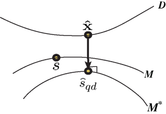
Figure 5. Information geometric picture of Inference 4 (imperfect observation and mismatched decoding).

Relationship between Inference with Partial Observed Data and Inference with Mismatched Decoding Model: Gaussian Case

In this section, we compute the Fisher information obtained by the four types of inference described in the previous section when the probability distributions are Gaussian. We also discuss the relationship between the inferences.

One-Dimensional Case

Before we deal with the multidimensional Gaussian model, we first consider the one-dimensional case as a toy example. We specifically consider the Gaussian distribution with mean μ(s) = s and variance σ²(s) = s²:

The statistical model M = {N(s, s²)} is expressed as a curve in the manifold S = {N(μ, σ²)} with coordinates of mean μ and variance σ² (Figure 6). The probability distribution on T observations of r is given by

where and are sufficient statistics

FIGURE 6

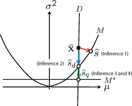
Figure 6. Information geometric picture of four types of inference in one-dimensional Gaussian model.

In this model, we compute the Fisher information and the information loss when the data of variance is lost and those when the decoding model whose variance is mismatched with the actual one is used.

Inference 1 When the data of neural responses are completely observed and the actual statistical model M is used in decoding, the maximum likelihood estimation of s corresponds to the orthogonal projection from to M (Figure 6). In this case, we can compute the Fisher information as

Inference 2 When data of variance is lost, the data manifold D is given by

In this case, the estimated value of s is the intersection point of D and M (Figure 6). By using Eq. 27, we can obtain the Fisher information,

where we used the fact that the marginal distribution over can be written as

can be derived by considering that also obey a Gaussian distribution and that the mean and the variance of are s and s²/T, respectively.

The information loss is given by

Inference 3 We specifically consider the inference with the following mismatched decoding model to compare it with the inference when is lost:

In this model, the mean is equal to the actual one but the variance is mismatched with the actual one. The maximum likelihood estimation based on the mismatched decoding model M* corresponds to the orthogonal projection from the observed point to M* (Figure 6). By using Eq. 36, we obtain the Fisher information

Inference 4 When the mismatched decoding model q(r), where the variance is independent of s, is used for decoding, the data of variance does not affect the results of the inference. Thus, even if is lost, no information is lost in this mismatched decoding. The Fisher information in the Inference 4 case is the same as that in the Inference 3 case:

As Eqs. 49 and 53 show, I_F3(s) is equal to I_F2(s). We can also easily show that I_F3(s) is equal to I_F2(s) in one-dimensional cases in general. However, in the multidimensional case, I_F3(s) is not equal to I_F2(s). In the next section, we explain the general relationship between I_F2(s) and I_F3(s) in the multidimensional Gaussian model.

Multidimensional Case

We next consider the multidimensional Gaussian distribution shown in Eq. 2. The probability distribution for T observations of neural responses r is given by

where the sufficient statistics and are

the natural parameters θ and Θ are

and the normalization constant Ψ(s) is

Inference 1 First, let us consider the Fisher information in the Inference 1 case. The Fisher information matrix with respect to the natural parameters is given by

By using the Fisher information matrix with respect to the natural parameters, we can obtain the Fisher information with respect to stimulus s from Eq. 25:

Inference 2 Second, let us consider the Fisher information in the Inference 2 case. We consider the situation that the second-order sufficient statistics in Eq. 55 are lost and only the first-order sufficient statistics are observed. The marginalized distribution over missing data is given by

where the natural parameters θ and Θ are

and the normalization constant Ψ(s) is

where we ignored the terms of the order of 1/T in the limit of T → ∞. In this case, the Fisher information matrix with respect to the natural parameters is computed as follows:

If we compare the components of the Fisher information matrix when is missing with those when the data are complete, the information loss due to the missing data is seen to be represented in the components (Eqs. 63 and 72). By using the Fisher information matrix with respect to the natural parameters, we can compute the Fisher information with respect to stimulus s as

From Eqs. 64 and 73, we find that the information loss due to the missing data is

This information loss solely depends on C′C⁻¹ and is always positive.

Inference 3 Third, let us consider the Fisher information in the Inference 3 case. In the Inference 2 case, we considered that the second-order sufficient statistics which are the variance and covariance data of neural responses, are lost. A mismatched probability distribution q(r; s) that is comparable with the inference when is lost would be that the mean in q(r; s) is the same as that in p(r; s) but the covariance matrix in q(r; s) does not match the true covariance matrix in p(r; s). As a simple example, we assume that the covariance matrix in the mismatched probability distribution is a constant matrix C_q that is independent of s:

In this case, we can show that the maximum likelihood estimation based on the mismatched probability distribution is consistent, i.e., the condition shown in Eq. 29 is satisfied, as follows:

By using Eq. 36, we obtain the Fisher information for the mismatched model q(r; s):

Inference 4 and comparison Finally, we consider the Fisher information in the Inference 4 case and compare the four types of inference described above. It is obvious that the Fisher information obtained by Inference 1, I_F1, is the largest and the Fisher information obtained by Inference 4, I_F4, is the smallest. On the other hand, the relationship between the Fisher information obtained by Inference 2, I_F2, and that obtained by Inference 3, I_F3, is not clear, i.e.,

However, the relationship between I_F2 and I_F3 can be clarified by considering the Fisher information obtained by Inference 4, I_F4. We assumed that a mismatched model that is related to the loss of covariance data, is the statistical model whose covariance matrix is a constant matrix. In this case, the vector of natural parameters Θ in Eq. 55, which is coupled with does not depend on s. Thus, when we use a mismatched model q(r; s) whose covariance matrix is independent of s, the inference does not change even if the data about covariance are lost. Thus, Inferences 3 and 4 result in the same estimate of s and the same Fisher information:

To summarize, the relationship between the Fisher information in each of the four inference cases is

Information Loss in Log-Linear Model of Binary Neural Response

In this section, we evaluate the information loss associated with loss of data and mismatched decoding in the log-linear model of binary neural response.

Two-Neuron Model

As the simplest example, we first consider the two-neuron model,

where Z(s) is a normalization constant,

The probability distribution for T observations of neural responses r can be written as

where and are sufficient statistics,

and is the number of configurations of (r⁽¹⁾, r⁽²⁾,…,r^(T)) where the sufficient statistics take the specific values can be expressed as

In the limit of T → ∞, by using Stirling’s formula, can be approximated as

Inference 1 We first compute the Fisher information in the Inference 1 case. The Fisher information matrix with respect to the natural parameters is given by

where 〈x〉 = E_p[x] = Σ_rxp(r₁, r₂). By using the Fisher information matrix with respect to the natural parameters, we can obtain the Fisher information with respect to stimulus s from Eq. 25:

Inference 2 We next compute the Fisher information when the data of neural correlation are lost. When T is finite, it is difficult to marginalize the probability distribution over because there are many possible when specific values of and are given. However, in the T → ∞ case, we only need to consider the most probable when and are given. By differentiating the argument of the exponential function in Eq. 83 with respect to we can obtain the equation for the most probable :

We denote the solution of this equation by Note that depends on Θ but does not depend on θ₁ and θ₂. The marginalized probability distribution is written as

By using Eq. 94, we can compute the Fisher information when is lost as

where we used the fact that only depends on Θ. The information loss is given by

This information loss only depends on ∂Θ/∂s. Thus, when Θ is independent of s, there is no information loss even if data are lost.

Inference 3 We next compute the Fisher information when neural correlation is ignored in decoding. We consider the mismatched decoding model q(r₁, r₂) that is the product of the marginal probability distributions of the actual distribution p(r₁, r₂):

where p(r_i) is the marginalized distribution over r_j, i.e., and the normalization constant is given by

From the definition of q(r₁, r₂), the averaged values of r₁ and r₂ over the mismatched model q(r₁, r₂) are equal to those over the actual model p(r₁, r₂). Thus, the following relationship holds between and the natural parameters in the actual probability distribution p(r₁, r₂):

The maximum likelihood estimation based on this mismatched decoding model q(r₁, r₂) is shown to be consistent as follows:

When the estimation by a mismatched decoding model is consistent, the Fisher information obtained by the mismatched decoding model can be computed by Eq. 36. The Fisher information is given by

where

As discussed in the previous section, I_F3(s) is always smaller than I_F2(s). Although the information loss associated with the loss of data only depends on ∂Θ/∂s, the information loss associated with ignoring correlation in decoding depends not only on ∂Θ/∂s but also on ∂θ₁/∂s and ∂θ₂/∂s. Thus, when neural correlation is ignored in decoding, the information is lost even if Θ is independent of s.

As a special case, if θ₁ = θ₂, which means 〈r₁〉 = 〈r₂〉 = 〈r〉, the information loss only depends on ∂Θ/∂s and is given by

In this case, ΔI_F3(s) is equal to ΔI_F2(s) (Eq. 96). This is because if θ₁ = θ₂ = θ, only two parameters, namely θ and Θ, are in the statistical model. This is the same situation as in the one-dimensional Gaussian case illustrated in Figure 6, where ΔI_F3(s) is also equal to ΔI_F2(s).

Homogeneous N Neuron Model

We next consider the case with a large number of neurons. In this case, the Fisher information cannot be analytically computed in general. To restrict ourselves to dealing with an analytically tractable model, we here only deal with a probabilistic model of a homogeneous neural population. In this model, θ_i(s) = θ(s) for any i and θ_ij(s) = Θ(s) for any pair of i and j, i.e.,

where the normalization constant Z(s) is given by

where Tr stands for the sum over all possible combinations of the neuron state variables (r₁, r₂,…,r_N). The probability distribution of T observations is given by

where and are sufficient statistics,

Inference 1 We first compute the Fisher information when data are complete and the decoding is optimal. As Eq. 23 shows, the Fisher information can be computed if we evaluate log Z. For analytical tractability, we consider the limit of N→∞. In this case, Z can be calculated as

where m is

and W(m) is the number of states where m takes a certain value, which is given by

In the limit of N→∞, by using Stirling’s formula, W(m) can be approximated as

We denote the argument of the exponential function in Eq. 110 by F, where

In the limit of N→∞, the integral in Eq. 110 can be approximated as

where F* is the maximum of the function F. From ∂F/∂m = 0, the value of m that maximizes the function F is the solution of the self-consistent equation

We set the solution of Eq. 116 to m*(θ, Θ). The Fisher information matrix with respect to the natural parameters θ and Θ is given by

By using the Fisher information matrix, we obtain the Fisher information with respect to stimulus s from Eq. 25:

Inferences 2 and 3 We next consider the situation where the data of correlation, , are lost and a mismatched decoding model that ignores neural correlation q(r; s) is used. We first consider the inference with a mismatched decoding model (Inference 3). This model q(r; s) is defined from the actual probability distribution p(r; s) as follows:

where the normalization constant Z_D is given by

The relationship between m* in the previous section and θ_D is

By comparing Eq. 123 with Eq. 116, we obtain

Similar to in the previous section, the maximum likelihood estimation with the independent decoding model q(r; s) can be shown to be consistent as follows:

By using Eq. 36, we can compute the Fisher information obtained by the independent decoding model as

Since I_F1(s) = I_F3(s) (see Eqs. 120 and 126), there is no information loss when the independent model is used for decoding in a homogeneous neural population (Wu et al., 2001). As for the Gaussian model, the Fisher information when the data of neural correlation are lost, I_F2, is larger than I_F3 and is smaller than I_F1. Since I_F1(s) = I_F3(s) in this case, I_F2(s) is also equal to I_F1(s). Thus,

In summary, no information is lost in a homogeneous neural population even when the data of neural correlation, , are lost or when the mismatched model that ignores neural correlation is used for decoding.

Discussion

In this work, we introduced a novel framework for investigating information processing in the brain where we studied information loss caused by two situations: imperfect observations and mismatched decoding. By evaluating the information loss caused by non-simultaneous observations of neural responses, we can quantify the importance of correlated activity. This can also be quantified by similarly evaluating the information loss caused by mismatched decoding that ignores neural correlation. We discussed these two types of loss by giving the information geometric interpretations of inferences with partially observed data and those with a mismatched decoding model and elucidated their relationship. We showed that the information loss associated with ignoring correlation in decoding is always larger than that caused by non-simultaneous observations of neural responses. This is because the inference based on an independent decoding model with complete data is equivalent to the inference based on an independent decoding model with “partial” data where the data of neural correlation are lost, which is naturally worse than the inference based on a correct decoding model with the partial data. This also can be intuitively understood by considering that decoding without the data of correlation considers all possible models of neural correlations, including the correct one, whereas decoding with a mismatched model locks it within the wrong domain.

Taking account of the relationship between the two inference methods, we give a simple guide on how to use the two different measures for quantifying the importance of correlation. To address the importance of coincidence detection by downstream neurons without making any specific assumption about the decoding process in higher-order areas in the brain, we should evaluate the information loss caused by non-simultaneous observations. The information loss quantified in this way can be used as the lower bound on the information conveyed by correlated activity. In contrast, the information loss quantified by using the independent decoding model can be used as the upper bound on the information conveyed by correlated activity because neural correlation is ignored not only in the observations but also in the decoding in this quantification. In summary, we consider that both measures should be computed when quantifying the importance of correlations and should be used as the lower bound and upper bound for the importance of correlations.

We considered the case that the stimulus is represented as a continuous variable. In this case, the Fisher information is a suitable measure for quantifying the maximal amount of information that can be extracted from neural responses. When considering a set of discrete stimuli, which is mostly the case for neurophysiological experiments, we should use the mutual information instead of the Fisher information. Similar to the Fisher information, the mutual information obtained by the inference with partially observed data can be computed by marginalizing the probability distribution of neural responses over the sufficient statistics that correspond to the lost data. In addition, the mutual information obtained by the mismatched decoding model can be computed using information derived by Merhav et al. (Merhav et al., 1994; Latham and Nirenberg, 2005; Amari and Nakahara, 2006; Oizumi et al., 2010). Thus, when we use the mutual information, we can also quantify the importance of correlation with the concepts of missing data and mismatched decoding. We analyzed the binary probabilistic model with a homogeneous neural population and found that neural correlation does not carry any information in this particular case. It is important to study how much information correlated activity could carry in an inhomogeneous neural population such as the hypercolumn model in V1. Another interesting future direction would be to evaluate the information conveyed by higher-order correlation (Amari et al., 2003); we considered only pair-wise correlation in this paper. These issues remain as future work.

Conflict of Interest Statement

The authors declare that the research was conducted in the absence of any commercial or financial relationships that could be construed as a potential conflict of interest.

Acknowledgments

This work was supported by a Grant-in-Aid for JSPS Fellows (08J08950) to Masafumi Oizumi. Masato Okada was supported by Grants-in-Aid for Scientific Research (18079003, 20240020, 20650019) from the Ministry of Education, Culture, Sports, Science and Technology of Japan.

References

Abbott, L. F., and Dayan, P. (1999). The effect of correlated variability on the accuracy of a population code. Neural. Comput. 11, 91–101.

Pubmed Abstract | Pubmed Full Text

Abeles, M. (1982). Role of the cortical neuron: integrator or coincidence detector? Isr. J. Med. Sci. 18, 83–92.

Pubmed Abstract | Pubmed Full Text

Amari, S. (1982). Differential geometry of curved exponential families – curvatures and information loss. Ann. Stat. 10, 357–385.

CrossRef Full Text

Amari, S. (1995). Information geometry of the EM and em algorithms for neural networks. Neural Netw. 8, 1379–1408.

CrossRef Full Text

Amari, S. (2001). Information geometry on hierarchy of probability distributions. IEEE Trans. Neural Netw. 47, 1701–1711.

Amari, S., and Nagaoka, H. (2000). Method of Information Geometry. New York: Oxford University Press.

Amari, S., and Nakahara, H. (2006). Correlation and independence in the neural code. Neural Comput. 18, 1259–1267.

Pubmed Abstract | Pubmed Full Text | CrossRef Full Text

Amari, S., Nakahara, H., Wu, S., and Sakai, Y. (2003). Synchronous firing and higher-order interactions in neuron pool. Neural. Comput. 15, 127–142.

Pubmed Abstract | Pubmed Full Text

Averbeck, B. B., Latham, P. E., and Pouget, A. (2006). Neural correlations, population coding and computation. Nat. Rev. Neruosci. 7, 358–366.

Averbeck, B. B., and Lee, D. (2006). Effects of noise correlations on information encoding and decoding. J. Neurophysiol. 95, 3633–3644.

Pubmed Abstract | Pubmed Full Text | CrossRef Full Text

Brunel, N., and Nadal, J. (1998). Mutual information, Fisher information, and population coding. Neural. Comput. 10, 1731–1757.

Pubmed Abstract | Pubmed Full Text

Ecker, A., Berens, P., Keliris, G., Bethge, M., Logothetis, N., and Tolias, A. (2010). Decorrelated neuronal firing in cortical microcircuits. Science 327, 584–587.

Pubmed Abstract | Pubmed Full Text | CrossRef Full Text

Gawne, T. J., and Richmond, B. J. (1993). How independent are the messages carried by adjacent inferior temporal cortical neurons? J. Neurosci. 13, 2758–2771.

Pubmed Abstract | Pubmed Full Text

Golledge, H. D., Panzeri, S., Zheng, F., Pola, G., Scannell, J. W., Giannikopoulos, D. V., Mason, R. J., Tovée, M. J., and Young, M. P. (2003). Correlations, feature-binding and population coding in primary visual cortex. Neuroreport 14, 1045–1050.

Pubmed Abstract | Pubmed Full Text | CrossRef Full Text

Gray, C. M., König, P., Engel, A. K., and Singer, W. (1989). Oscillatory responses in cat visual cortex exhibit inter-columnar synchronization which reflects global stimulus properties. Nature 338, 334–337.

Pubmed Abstract | Pubmed Full Text | CrossRef Full Text

Ishikane, H., Gangi, M., Honda, S., and Tachibana, M. (2005). Synchronized retinal oscillations encode essential information for escape behavior in frogs. Nat. Neurosci. 80, 1087–1095.

König, P., Engel, A. K., and Singer, W. (1996). Integrator or coincidence detector? The role of the cortical neuron revisited. Trends Neurosci. 19, 130–137.

Pubmed Abstract | Pubmed Full Text | CrossRef Full Text

Latham, P. E., and Nirenberg, S. (2005). Synergy, redundancy, and independence in population codes, revisited. J. Neurosci. 25, 5195–5206.

Pubmed Abstract | Pubmed Full Text | CrossRef Full Text

Lee, D., Port, N. L., Kruse, W., and Georgopoulos, A. P. (1998). Variability and correlated noise in the discharge of neurons in motor and parietal areas of the primate cortex. J. Neurosci. 18, 1161–1170.

Pubmed Abstract | Pubmed Full Text

Meister, M., Lagnado, L., and Baylor, D. A. (1995). Concerted signaling by retinal ganglion cells. Science 270, 1207–1210.

Pubmed Abstract | Pubmed Full Text | CrossRef Full Text

Merhav, N., Kaplan, G., Lapidoth, A., and Shamai Shitz, S. (1994). On information rates for mismatched decoders. IEEE Trans. Inf. Theory 40, 1953–1967.

Montani, F., Ince, R. A. A., Senetore, R., Arabzadeh, E., Diamond, M., and Panzeri, S. (2009). The impact of higher-order interactions on the rate of synchronous discharge and information transmission in somatosensory cortex. Philos. Trans. R. Soc. A 367, 3297–3310.

Nakahara, H., and Amari, S. (2002). Information-geometric measure for neural spikes. Neural. Comput. 14, 2269–2316.

Pubmed Abstract | Pubmed Full Text

Nirenberg, S., Carcieri, S. M., Jacobs, A. L., and Latham, P. E. (2001). Retinal ganglion cells act largely as independent encoders. Nature 411, 698–701.

Pubmed Abstract | Pubmed Full Text | CrossRef Full Text

Nirenberg, S., and Latham, P. E. (2003). Decoding neural spike trains: how important are correlations? Proc. Natl. Acad. Sci. U.S.A. 100, 7348–7353.

Pubmed Abstract | Pubmed Full Text

Ohiorhenuan, I. E., Mechler, F., Purpura, K. P., Schmid, A. M., Hu, Q., and Victor, J. D. (2010). Sparse coding and high-order correlations in fine-scale cortical networks. Nature 466, 617–622.

Pubmed Abstract | Pubmed Full Text | CrossRef Full Text

Oizumi, M., Ishii, T., Ishibashi, K., Hosoya, T., and Okada, M. (2010). Mismatched decoding in the brain. J. Neurosci. 30, 4815–4826.

Pubmed Abstract | Pubmed Full Text | CrossRef Full Text

Schneidman, E., Berry, M. J. II, Segev, R., and Bialek, W. (2006). Weak pairwise correlations imply strongly correlated network states in a neural population. Nature 440, 1007–1012.

Pubmed Abstract | Pubmed Full Text | CrossRef Full Text

Shlens, J., Field, G. D., Gauthier, J. L., Grivich, M. I., Petrusca, D., Sher, A., Litke, A. M., and Chichilnisky, E. J. (2006). The structure of multi- neuron firing patterns in primate retina. J. Neurosci. 260, 8254–8266.

Tang, A., Jackson, D., Hobbs, J., Chen, W., Smith, J. L., Patel, H., Prieto, A., Petrusca, D., Grivich, M. I., Sher, A., Hottowy, P., Dabrowski, W., Litke, A. M., and Beggs, J. M. (2008). A maximum entropy model applied to spatial and temporal correlations from cortical networks in vitro. J. Neurosci. 28, 505–518.

Pubmed Abstract | Pubmed Full Text | CrossRef Full Text

Wu, S., Nakahara, H., and Amari, S. (2001). Population coding with correlation and an unfaithful model. Neural Comput. 13, 775–797.

Pubmed Abstract | Pubmed Full Text | CrossRef Full Text

Yaeli, S., and Meir, R. (2010). Error-based analysis of optimal tuning functions explains phenomena observed in sensory neurons. Front. Comput. Neurosci. 4:130. doi: 10.3389/fncom.2010.00130

Pubmed Abstract | Pubmed Full Text | CrossRef Full Text

Zohary, E., Shadlen, M. N., and Newsome, W. T. (1994). Correlated neuronal discharge rate and its implications for psychophysical performance. Nature 370, 140–143.

Pubmed Abstract | Pubmed Full Text | CrossRef Full Text