Methods for generating complex networks with selected structural properties for simulations: a review and tutorial for neuroscientists

1 Introduction

Recent advances in imaging techniques have led to improved data, and increased knowledge, about the connectivity of both structural (anatomical) and functional networks in the brain (Bullmore and Sporns, 2009). Many studies across a diverse range of anatomical parts of the brain and scales have found that networks may exhibit complex connectivity properties. By complex, we mean that they display inhomogeneous features characteristic of a combination of both regularity and randomness – see Bullmore and Sporns (2009) for a comprehensive review, and Buzsáki (2006); Sporns (2011) for further discussion. These include so-called “scale-free” networks (Freeman and Breakspear, 2007) and/or “small-world networks” (Bassett and Bullmore, 2006; He et al., 2007).

The feature that distinguishes any network with either (or both) of these properties, from ordered or regular networks, and what are usually simply called “random networks,” is that scale-free (Barabási and Albert, 1999) networks are inhomogeneous in the “degree” of nodes (i.e., the number of connections a node has to other nodes), and small-world networks (Watts and Strogatz, 1998) are inhomogeneous in that the pattern of connectivity between nodes is relatively localized. By contrast, regular and random networks are statistically completely homogeneous in both properties. Differences like these are referred to as differences in network topology.

While such complex network topologies have been studied in neural models by simulation or in terms of their statistical physics (Roxin et al., 2004; Shanahan, 2008), the recent acceleration of experimental evidence in favor of their existence in the brain at multiple scales lead us to anticipate that many more modeling studies will be forthcoming. These will, for example, attempt to replicate topologies observed in data, and be aimed at attempting to understanding how structural networks are related to functional networks (Sporns, 2011).

Despite it being recognized for some time that networks in the brain can be both scale-free and small-world in their connectivity (Buzsáki, 2006), many simulations, e.g., of cortical neuronal networks, have assumed completely homogenous regular or random networks. In order to highlight that simple algorithms exist for incorporating complex heterogeneity in simulations, in this paper we review the most well known ones.

Scientific analysis of the connectivity properties of networks is facilitated by a field of mathematics known as graph theory (Newman et al., 2006). We therefore also review mathematical results that can be readily used to help verify correct implementation. Many expressions describing statistical properties of networks have been obtained by the statistical physics community (Albert and Barabási, 2002; Newman, 2003; Boccaletti et al., 2006; Newman et al., 2006), but the majority are only approximations or asymptotic, even though they are sometimes stated as apparently exact results. This can lead to confusion when simulation results are not in agreement with the theory.

Our intention is to provide a resource that a reader can use to help them confidently write software that produces a network which they can state conforms to a given algorithm and/or network properties and statistics, and then adapt as necessary. Such a resource is an essential prerequisite for many kinds of simulations, such as comparative studies of whether certain network structures are essential for aspects of brain functionality.

1.1 Network Models Covered in this Paper

Many well known networks, e.g., the internet, social networks, and neuronal networks, are easily characterized as graphs using the terminology and notation of the field of graph theory. Such graphs consist of a set of N nodes and K edges.

The first network we describe, that of Erdös and Rényi (1960), is extremely well known, and dates back to the 1950s, when considerable research was being carried out into graph theory, and its suitability for modeling real world networks. Perhaps it is worth remembering that at that time computers were a rare luxury when it came to modeling such networks, and even on those occasions one was available, its “computing power” was almost insignificant compared to modern systems. As a consequence much of the modeling was based on relatively small “ordered” or “regular” networks. Such networks are rare in the real world, and consequently Erdös and Rényi (1959, 1960) produced two random graph models, the G(N, M) and G(N, p) models, while working separately Gilbert (1959) also produced the G(N, p) model.

The G(N, M) model uniformly randomly selects a graph from the set of all possible graphs with N nodes and M edges. The G(N, p) model connects each distinct node pair with probability p – we will consider only this model. What these models show is that random networks have a consistently shorter average path length than ordered networks.

This was the first major step in solving three main problems in using graph theory to model real world complex networks. Two other main inconsistencies remained. The second is the tendency of nodes in real world networks to form highly interconnected groups, or clusters, and yet still retain irregular connectivity patterns. The model of Watts and Strogatz (1998) captures these features, and is therefore the second network we consider.

The third inconsistency is that neither the Erdös–Rényi network nor the Watts and Strogatz (1998) network reproduce networks with “hubs” – i.e. a small number of nodes with a much larger than average number of edges to/from other nodes – or a property known as “scale-free.” The model of Barabási and Albert (1999) does, and we thirdly consider this model, although note that it does not reproduce the small-world property of Watts and Strogatz (1998).

The final specific network that we discuss in full detail is a lesser known network generation algorithm – although it is reviewed in Boccaletti et al. (2006) – that of Klemm and Eguílez (2002b), which leads to networks that are both scale-free, and small-world.

Another class of network structure that is also relatively less well known in many application areas for graph theory, but is of high relevance for neuroscience modeling (Meunier et al., 2010) is modular networks (Girvan and Newman, 2002).

We note that there are many variations that can be added to the models reviewed here that may provide networks with desired statistics – see, for example Newman et al. (2006) for reviews. In particular, we do not discuss weighted networks, as our intention is to introduce the basic concepts and ideas.

1.2 Organization of Paper

The remainder of this paper is organized as follows. In Section 2 we introduce and discuss relevant graph theoretic terminology and statistics. Next, Section 3 contains descriptions and pseudo-code for the four network generation algorithms we are focusing on, as well as stating known mathematical results for the resultant networks. Example simulations and use of mathematical results are given in Section 4. Finally, in Section 5 we briefly discuss other metrics and networks types that we have not covered in this paper, as well as some of the limitations and caveats of comparing simulated networks to data.

2 Terminology and Commonly Used Network Statistics

In this section we discuss three of the most widely known metrics used for characterizing network topology: degree distribution, average path length, and clustering coefficient. This allows us to define “small-world” and “scale-free.” Table 1 summarises the mathematical notation we introduce. Firstly we introduce some terminology and discuss the crucial aspect of network directedness.

TABLE 1

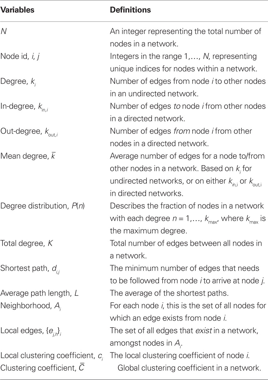
Table 1. Quick reference guide for mathematical notation used to describe graphs and associated statistics.

2.1 Directed and Undirected Networks

Graphs may be directed or undirected. This is important for communication processes between nodes in a network. If a graph’s nodes are indexed between 1 and N, each edge is defined as a link between a pair of nodes, say i and j. In an undirected graph, the ordering of the pair of nodes that define each edge is unimportant: if an undirected edge links nodes i and j, then node i can communicate to node j and node j can communicate to node i. In a directed graph, the ordering is meaningful: if there exists a directed edge from node i to node j, node i can communicate to node j. However, unless there exists a corresponding directed edge from node j to node i, node j cannot communicate directly to node i. As will be discussed later in the paper, this has a considerable impact when choosing a domain appropriate model for simulations.

To avoid confusion, in pseudo-code presented below we will refer to the connections between node pairs in undirected networks as reciprocal edges and to those in directed networks as directed edges, with a postfix similar to “from i to j,” so as to clearly define direction of possible communication.

2.2 Adjacent and Neighborhood

Two nodes in an undirected network are said to be adjacent if an edge that links the two nodes exists. In a directed network, node i is said to be adjacent to node j (and node j is said to be adjacent from node i) if a directed edge from node i to j exists. If there is no directed edge from node j to node i, than node j is not adjacent to node i.

The neighborhood, A_i, of node i is defined as the set of all nodes j that are adjacent from node i. Each node in a neighborhood, A_i is called a neighbor of node i. There is an important (and domain specific) distinction when modeling with directed networks, as the neighborhood only includes nodes j when there exists a directed edge from node i. That is, j to i only edges are not in the neighborhood A_i.

2.3 Degree, Mean Degree and Degree Distribution

The degree of node i in an undirected graph, denoted as k_i, is the number of edges between node i and other nodes in the graph, i.e., the size of the neighborhood, A_i. If a network is directed then each node will have both an in-degree and an out-degree. For such networks, we introduce the notation k_{in, i} and k_{out, i} to denote these for node i.

The mean degree of an undirected network, is simply the average of the nodal degrees:

For a directed network we have mean in-degree (denoted as ) and mean out-degree (denoted as ).

Degree distribution refers to the probability P(n) that an arbitrarily selected node in a network has degree n, where n = 1, …, k_max, and k_max is the maximum degree. If a network is directed then it has in-degree and out-degree distributions. Equivalently, the term is used to describe the fraction of nodes in a network with degree, n. For empirical networks it can be found as follows. Let κ_n be a count of the number of nodes in a network with degree n, where n = 1, …, k_max. The degree distribution is given by P(n) = κ_n/N.

For networks whose properties are based on theoretical algorithms, P(n) can be derived mathematically, and refers to the probability that an arbitrary node, out of all possible networks that the algorithm can generate, has degree n. The degree distribution of a single instance of such a network is only an approximation to the mathematical derivation, but is usually more accurate as N increases.

2.4 Average Path Length

Average path length is one of the most commonly used metrics for quantifying network topology (Albert and Barabási, 2002). It has important implications for the study of how neuronal networks are “wired,” as well as their ongoing evolution (Buzsáki, 2006; Achard and Bullmore, 2007; Bullmore and Sporns, 2009).

Mathematically, we denote average path length of a graph as L. It is defined as the average number of edges that must be traversed in the shortest path d_i,j between any two pairs of nodes i and j. Shortest path is defined as the minimum number of edges that must be followed from node i to arrive at node j. If we define d_i,j = 0 when i = j or there is no path between i and j, then this can be expressed as

where the term N(N − 1) is the total number of node pairs.

Note that this expression is true for both directed and undirected graphs, but that since it is always true that d_i,j = d_j,i for undirected graphs, the expression simplifies in this case to

The topology of a network has a profound effect on the way average path length scales with network size, N. For example, for a regular ring lattice topology (see Figure 1), L scales linearly, whereas with a Barabási and Albert (1999) scale-free network it scales logarithmically. For the small-world network of Watts and Strogatz (1998), the scaling of L with N is dependent on a parameter used in the construction of the network – see Section 3.

FIGURE 1

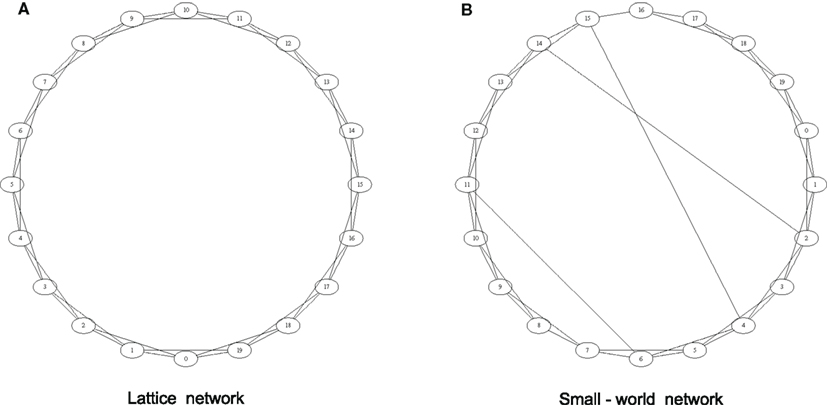
Figure 1. The Watts and Strogatz (1998) algorithm begins with a ring lattice network (A), which is a ring of nodes with edges divided evenly between its k_L closest left and right neighbors. The lattice is converted to a small-world network (B) by the algorithm of Watts and Strogatz (1998). Here we used p_w = 0.05, k_L = 4, and N = 20.

2.4.1 When is average path length a useful metric?

Average path length can be a somewhat problematic metric, because in some contexts it is only meaningful for graphs where all N nodes can be reached from any other node in the network. Graphs where this is not true are described as not connected. Here we define as zero the shortest path between pairs of nodes for which no path exists, so that L can be calculated. We do this because all the networks we consider are either guaranteed to allow all paths to exist, or produce networks where the probability that paths between node pairs do not exist is infinitesimal.

Whether this is a useful approach for other networks depends on what is being modeled. If for example the network being modeled will potentially contain disconnected node pairs, and disconnected nodes affect what is being modeled, it might be helpful to find a metric that will identify and assess such a topology. One option would be global efficiency or average inverse shortest path – see Boccaletti et al. (2006) for a review of such alternative metrics. Another alternative is to simply calculate a vector of average path lengths for each separate sub network of the overall network.

2.5 Clustering Coefficient

Clustering coefficient is a statistic introduced originally by Luce and Perry (1949) that describes the likelihood that any node j in the neighborhood, A_i, of node i, is also adjacent to the other nodes in A_i. It later became a focus point in Watts and Strogatz’ seminal work highlighting the important convergence of two factors, short average path length, and high clustering coefficient (Watts and Strogatz, 1998).

The tendency for a higher likelihood of j being adjacent to h when both j and h are in A_i, compared with when h is an arbitrary node selected from all other nodes in the network, is a phenomenon which has been noted in many designed and naturally occurring complex networks (Milgram, 1967; Watts and Strogatz, 1998). In particular, a high level of clustering has been observed in anatomical connections between brain regions (Buzsáki, 2006; Bullmore and Sporns, 2009).

Several methods exist for measuring clustering coefficient. One of the first was the “triangles” method (Luce and Perry, 1949), which uses the ratio between open and closed triangles to calculate clustering coefficient. The method of Soffer and Vázquez (2005) was created to exclude degree correlation biases. It is important to be aware of the different choices available, and to chose the most appropriate method for the application – see also (Newman et al., 2002; Barrat et al., 2004; Schank and Wagner, 2005).

We shall use the Watts and Strogatz (1998) definition of clustering coefficient, because it is widely used, intuitive and it can provide local as well as global clustering coefficients. With this definition, local clustering coefficient, c_i for node i is defined as the fraction of actual edges between node i’s neighbors, out of all possible edges between its neighbors. The (global) clustering coefficient, is simply the average of the N local clustering coefficients. While this metric is primarily used only for undirected networks – see Section 2.5.1 – it is simple to naively extend it to undirected networks by considering either only the outward edges or only the inward edges of each node to be actual connections. Note that the total number of possible edges in i’s neighborhood, A_i, for undirected graphs is k_i(k_i − 1)/2 and for directed graphs is k_out,i(k_out,i − 1).

To write an expression for local clustering coefficient, we introduce the notation {e_j,h}_i to denote the set of all edges that exist in a network, amongst nodes in A_i. The indices j and h are in the ranges j = 1,…,k_i, h = 1, …, k_i, j ≠ h for undirected networks and j = 1, …, k_out,i, h = 1,…,k_out,i, j ≠ h for directed networks. The size of the set of edges is denoted as |{e_j,h}_i|.

For undirected networks the local clustering coefficient is

For directed networks the local clustering coefficient based on outward edges is

A similar expression may be written for inward edges.

The global clustering coefficient is

Note that

2.5.1 When is clustering coefficient a useful metric?

As stated above, the clustering coefficient of Watts and Strogatz (1998) was designed to be used as a statistic for undirected networks. While it is mathematically simple to extend it to directed networks the meaningfulness of doing so is less clear, and depends on what is being modeled. For example, it might be considered as a form of clustering if nodes that are adjacent from node i are likely to have at least one directed edge between them. The directed definition we stated above is not suited to measuring this, because edges in both directions contribute double a single directed edge. Nor does it take into account whether clustering for directed networks should be defined in a way that emphasizes the existence of bidirectional links, i.e., where nodes i and j have directed edges both from i to j and j to i – see Song et al. (2005) for experimental evidence of the existence of such links in the rat visual cortex. Resolving the question of the most appropriate definition of clustering coefficient for such directed networks is beyond the scope of this tutorial/review paper – see Fagiolo (2007) for two alternative definitions of clustering coefficient for directed networks, and associated discussion. See also Rubinov and Sporns (2010).

2.6 Small-World Networks and Proximity-Ratio

It is difficult to identify a consensus on how exactly to define “small-world” for the purposes of classifying a network. As pointed out by Newman et al. (2006), “the small-world effect” is a term used to describe networks whose average path length is comparable with a homogeneous random network, without any regard to clustering. On the other hand, the specific network generation algorithm described by Watts and Strogatz (1998) leads to what they call a small-world network when the clustering coefficient is large compared to that of a random network, and the average path length is comparable to that of a random network. This definition is satisfactory for that network, because the actual magnitude of the clustering coefficient is clearly comparable with a regular network that conforms with an intuitive definition of clustering.

However, the definition of Watts and Strogatz (1998) can be problematic if one attempts to use it to classify arbitrary networks. For example, it is shown below that the clustering coefficient of the scale-free network of Barabási and Albert (1999) decreases as the network size increases, but that the rate of decrease is slower than that of a random network. In this sense, the clustering coefficient of the former network is much larger than that of the latter, which by Watts and Strogatz (1998) would mean classifying the scale-free network as “small-world.” This contradicts the fact that the clustering coefficient is extremely small relative to regular lattices.

One suggested approach to avoiding such ambiguity is to quantify the “small-world-ness” of a network, as suggested by Walsh (1999), and who to this end introduced a metric known as proximity-ratio. This is defined as

where _r and L_r are the clustering coefficient and average path length of a random network with the same size, N, and mean degree, k, of a network with clustering coefficient and average path length L. With these definitions, the Watts and Strogatz (1998) definition requires that and Walsh (1999) defines a network as “small-world” when S ≫ 1, given that S = 1 for a random network, and this definition agrees with that of Watts and Strogatz (1998), but additionally provides a means of quantitatively comparing networks.

This metric has recently been independently defined in neuroscience in order to quantify the “small-world-ness” of neural circuits in the brain stem (Humphries et al., 2006), who in contrast to Walsh (1999) suggest S > 1 and suffices to identify a small-world network.

2.7 Scale-Free Networks

While degree distribution has long been of interest in the study of complex networks (Erdös and Rényi, 1960; Price, 1965), it was more recently brought to prominence in Barabási and Albert’s (1999) ground breaking work on constructing scale-free networks. A scale-free network has a degree distribution where the probability of a node having a given degree has a scale-invariant decay as degree grows. That is, it follows a power-law of the form

where γ > 1 is a constant and n = 1, 2,…, N. As is discussed in more detail below, such a distribution is very different to that of homogeneous random networks.

Scale-free degree distributions appear in complex systems throughout the natural world, as well as in designed systems. It is not yet clear whether scale-free degree distributions can be expected to be prevalent in brain networks (Sporns, 2011) at all scales. However, “hubs” and “power-law” degree distributions have been observed, and how they develop and their role in brain function are an important area of research (Buzsáki, 2006).

3 Simulating Complex Brain Networks with and without Small-World and/or Scale-Free Properties

In this section we present three very well known networks, and one less well known network. Table 2 summarises the parameters that need to be selected when generating these networks. The first network, usually attributed to Erdös and Rényi is probably the single most widely used model. It is often referred to as a “random network,” and it sets a benchmark for homogeneity, based on three characteristic properties: (i) its degree distribution symmetrically decays away from the mean degree; (ii) its average path length increases as the network size increases for a fixed mean degree; and (iii) it has a clustering coefficient that reduces as the network size increases for a fixed mean degree.

TABLE 2

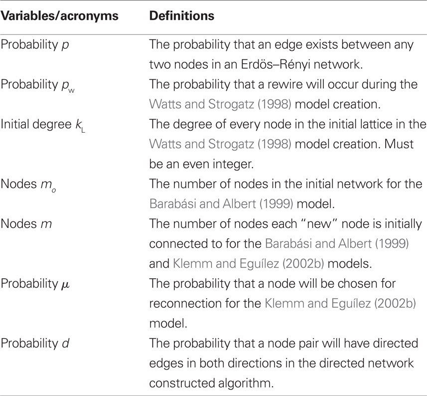
Table 2. Quick reference guide for parameters within the discussed network generation algorithms.

The second network we consider is the “small-world” network of Watts and Strogatz (1998). While the degree distribution of this network is similar to that of an Erdös–Rényi random network – in the sense that it has a central peak at the mean degree and degree probabilities that rapidly decrease for degrees away from the mean, which is very dissimilar to scale-free degree distributions – the network’s clustering coefficient is large compared with an Erdös–Rényi random network of the same size and mean degree, and is almost independent of N, while the average path length increases with network size at about the same rate as an Erdös–Rényi random network of the same size and mean degree. Thus, the network is inhomogeneous in the sense that nodes in the neighborhood of any node i are more likely to be in the neighborhood of each other than they are in an Erdös–Rényi random network.

The third network is the scale-free network described by Barabási and Albert (1999). This network is quite unlike the Erdös–Rényi random network because it contains large numbers of nodes with small degree, and a small numbers of “hubs,” which are nodes with very large degree. Thus the degree distribution is highly inhomogeneous. The average path length and clustering coefficient both change with the network size in a manner similar to the Erdös–Rényi random network.

The fourth network (Klemm and Eguílez, 2002b) is less well known, but we present it here because it combines the high local clustering of the Watts–Strogatz small-world network, and the degree distribution of the Barabási–Albert scale-free network, and can therefore be described as a scale-free small-world network.

Apart from the Erdös–Rényi random network, which is often easily converted to a directed network, the other networks described are usually undirected only. But, as discussed, structural and functional brain networks may be either directed or undirected. For example, at the scale of communication between individual neurons, a directed network is a good model, because action potentials that initiate in one neuron propagate from that neuron along axons, where they cause changes in the state of other neurons via synaptic junctions. In contrast, at the scales of imaging techniques like fMRI, EEG, and MEG, functional and structural networks can be inferred that are best modeled as undirected networks. Nodes in these models consist of gross areas of the brain that consist of millions of neurons, and edges represent the fact that two way communication must exist between those nodes.

We therefore in the pseudo-code describe for each network one simple switch that converts the original network to a directed network. This suggested conversion is by no means the only or best conversion – we chose our approach for simplicity, minimal change, and to ensure the directed network has very close to the same statistical properties as the corresponding undirected network. In particular, we ensure the mean in-degree and mean out-degree of the directed networks are both the same as the mean degree of the corresponding undirected network.

Each conversion to a directed network is tailored to the network topology it is modifying, and employs a variable d that determines the probability that modified edges are undirected equivalent, i.e., whether they are reciprocal. For example in the case of d = 1, all modified edges are reciprocal and as such there is no practical difference between the directed and the undirected version. However, we introduce d so that in general it can be set to less than 1 and thus result in non-trivial conversions where there exist node pairs that may not be connected in both directions; e.g., we have found that d = 0.5 does not significantly affect the metrics we discuss in this paper. However, otherwise the influence of d on statistical parameters is beyond the scope of this paper, as it is our intention to highlight the need to consider directed networks, without regard to the generic properties of the example approach we use to illustrate this fact.

Note that the factor d does not have the same influence on all of the networks discussed. It is only applied to the “randomization” section of the Watts–Strogatz model; as such it will only affect edges that have been re-wired, which is generally a very small proportion of total edges; the remainder of the network maintains its undirected equivalence.

3.1 Erdös–Rényi Random Network

The following algorithm produces a G(N, p) Erdös–Rényi random network with mean degree or if desired, our directed version of it, which is designed to mirror as closely as possible the directed extensions of the other three networks presented below. In this algorithm all possible edges are considered and included in the network with probability p.

For: each node i
  For: each node j = i + 1…N
    Set: Chance = a uniform random number between 0 and 1
      If: p > Chance
        If: Undirected
          Create a reciprocal edge between node i and node j
        Else
          Set: Chance = a uniform random number between 0 and 1
          If: d > Chance
            Create a directed edge from node i to node j
            Create a directed edge from node j to node i
          Else
            Create a directed edge from node i to node j
            Set: Node h : uniformly randomly chosen from the set of all nodes excluding i and j
          Create a directed edge from node h to node i
          EndIf
        EndIf
      EndIf
    EndFor
  EndFor

3.1.1 Mathematical verification for (undirected) Erdös–Rényi random networks

The degree distribution of an undirected Erdös–Rényi G(N, p) random network is well known to be the binomial distribution,

The mean degree for a network with m edges is It is quite common to use large graphs, i.e., where N is large. In this case it can be shown that the degree distribution is well approximated by the Poisson distribution, provided p is sufficiently small, i.e., Under these conditions we have

There is no known exact result for the average path length of this undirected network. A widely known scaling relationship (Watts and Strogatz, 1998; Albert and Barabási, 2002) can be used to provide qualitative guidance on how L changes with the network size and mean degree:

This scaling relationship says that for fixed mean degree, the average path length is expected to increase logarithmically with network size. Less well known is an approximation to the average path length due to Fronczak et al. (2004), which states that for N sufficiently large and

The Watts–Strogatz clustering coefficient of an undirected Erdös–Rényi random network is given by (Watts and Strogatz, 1998; Albert and Barabási, 2002)

3.2 Watts–Strogatz Small-World Network

While experimenting with just how much randomness was required to substantially reduce the average path length of regular networks, Watts and Strogatz (1998) created what has become known as the archetypical small-world network. They began by creating an undirected ring lattice network – see Figure 1A. These networks have a high clustering coefficient in comparison to Erdös–Rényi random networks, i.e., if each node has a degree k_L, where k_L is even, then (Barrat and Weigt, 2000).

They then applied a process of random rewiring, whereby each edge has an arbitrarily chosen probability, p_w, of being re-wired – see Figure 1B. Note that (i) the algorithm rewires only one end of each edge, and traverses edges in a manner that ensures each node loses at most half of its edges; and (ii) edges are only replaced, not added or removed and therefore the total number of edges and the mean degree is unchanged. By varying p_w they were able to show that only a very small number of “rewires” is required to produce a low average path length (i.e., comparable to that of an Erdös–Rényi random network of the same size and mean degree), whilst maintaining a high clustering coefficient (i.e., comparable to the lattice, and much larger than that of an Erdös–Rényi random network of the same size and mean degree).

The reason that only a few re-wirings can cause such a dramatic change in average path length, and hardly affect clustering coefficient, is that by definition, the clustering coefficient is a global metric based on the average of local clustering coefficients. Thus, a small number of re-wirings will only affect a small number of terms in the average, and not change it significantly. However, each term in the average path length is a global metric – the shortest path between each pair of nodes. One changed link has the potential to significantly change a large number of shortest paths by creating “shortcuts,” and thus lead to a significant change in average path length.

These network characteristics dealt with the second major problem for the modeling of real world networks as outlined in Section 1. However, as each “rewire” is random and merely occasionally replaces a close neighbor with a long distance one (introducing a “shortcut” effect) the reduction of average path length is affected without any change to average degree, and without creating degree distributions with hubs or the scale-free property. It is noted that there is no guarantee that an immediate neighbor will be replaced with one more “distant” – i.e., one for which the current shortest path is relatively long – it is simply that in a network with it is statistically more likely that the new neighbor will be outside a node’s neighborhood. It is further noted that the degree distribution will be affected, in correlation with the size of p_w (i.e., the number of random rewires).

The following algorithm produces the undirected Watts and Strogatz (1998) small-world network of size N, or if desired, our directed version of it. The parameters are k_L, the total number of edges for each node in the initial network (assumed to be even), and p_w, the rewiring probability. Note that the algorithm ensures each edge in the initial ring lattice is considered for rewiring exactly once.

//First create a ring lattice
For: all nodes i = 1…N
  For: all nodes j = i + 1…i+ κL/2
    If: j > N //Make sure forward connects loop round
      Set: j = j − N ;
    EndIf
    If: Undirected
      Create a reciprocal edge between node i and node j
    Else
      Create a directed edge from node i to node j
      Create a directed edge from node j to node i
    EndIf
  EndFor
EndFor
//Second rewire edges randomly with probability pw
For: all nodes i = 1…N
  For: all nodes l = i + 1…i+ κL/2
    If: l > N //Make sure forward connects loop round
      Set: l = l − N ;
    EndIf
    Set: Chance = a uniform random variable between 0 and 1
      If: pw > Chance
        Set: node j = uniformly randomly chosen from the set of all nodes, excluding i and nodes adjacent to/from i other than j
          Disconnect: node i and node l
        If: Undirected
          Create a reciprocal edge between node i and node j
        Else
          Set: Chance = a uniform random number between 0 and 1
          If: d > Chance
          Create a directed edge from node i to node j
          Create a directed edge from node j to node i
        Else
        Create a directed edge from node i to node j
          Set: Node h : uniformly randomly chosen from the set of all nodes excluding i, j and nodes adjacent to i
          Create a directed edge from node h to node i
        EndIf
      EndIf
    EndIf
  EndFor
EndFor

3.2.1 Mathematical verification for the (undirected) network of Watts and Strogatz (1998)

Although the mean degree is exactly (Barrat and Weigt, 2000), no exact expression for the degree distribution for a Watts–Strogatz small-world network is known, except when p_w = 0, in which case every node has degree k_L. An approximation for the case of 0 < p_w < 1 was calculated by Barrat and Weigt (2000) as

where . Note that k_L is assumed to be even and therefore the argument in the factorial (n − k_L/2 − i)! is always integer. Like the Erdös–Rényi random network, this degree distribution has a peak at the mean degree, and tails off for larger and smaller degrees. The network could perhaps therefore be considered homogeneous for degree, except for the fact that the construction algorithm does not allow nodes to have a degree smaller than k_L/2.

There is also no known exact expression for average path length of this network. A scaling approximation due to Newman et al. (2000) is that

where u = p_wk_LN. For the case of fixed p_w and k_L, if and N is sufficiently large, then the average path length is expected to increase with network size, because the terms involving u converge to a constant for large N (Albert and Barabási, 2002).

While clustering coefficient also does not have a known exact expression, it was shown by Barrat and Weigt (2000) that it is well approximated for large N as

Since N is assumed to be large, for p_w < 1 the term expressed as O(1/N) can be ignored.

As discussed in Section 2.6, Watts and Strogatz (1998) evaluate their network relative to an Erdös–Rényi type random network. Suppose p < 1, and that an Erdös–Rényi random network has size N and mean degree k_L = κ, and a Watts and Strogatz (1998) network also has size N and parameter k_L = κ, where N ≫ κ. With reference to Eqns (9) and (12), one of the two requirements of the Watts and Strogatz (1998) definition of a small-world means that

As discussed by Watts and Strogatz (1998), the stated condition can be shown numerically to be true for a broad range of p_w > 0.

Another interesting difference between the clustering coefficients of the two models is that as N increases, the clustering coefficient for the Watts and Strogatz (1998) network is almost independent of N for p_w < 1, while it decreases inverse proportionally with N for the Erdös–Rényi network. This term O(1/N) in Eqn. (12) is only significant when p_w → 1, in which case both networks show the same scaling with N. These facts should be observable from any simulation of these networks.

Finally, we remark that despite similar clustering coefficients and average path lengths, a Watts and Strogatz (1998) network with p_w = 1 is not identical to an Erdös–Rényi random network with the same size and mean degree since, for example, the Watts–Strogatz algorithm does not allow nodes to exist with degree smaller than k/2, whereas that of Erdös–Rényi does.

3.3 Barabási and Albert Scale-Free Network

In their ground breaking work Barabási and Albert (1999) noted that many “real world” networks such as citation networks, the world wide web, and biological networks have hubs, that is, a small number of nodes with a very large degree. One possible factor for the ubiquity of network topologies that contain hubs is that they have been shown to be more robust when faced with non-targeted node removal (Barabási and Albert, 1999). It is possible that this offers an advantage for such topologies in naturally evolving networks. Barabási and Albert (1999) hypothesized that part of the reason for the existence of such networks is due to a preferential attachment bias, i.e., the “rich-get-richer” phenomena, whereby nodes with the largest degree are more likely to attract connections from nodes being added to the network. Accordingly they designed a network generation model which incorporates such a bias by assigning each existing node a probability of receiving new edges proportional to its current degree.

The resultant network topology follows a power-law degree distribution like that introduced in Eqn. (5). As such, it has resolved the final of the three problems with compatibility between network generation models, and “real world” network topologies, as described in Section 1. However, as is shown below, while its average path length is comparable to a random network, it does not exhibit high local clustering. Nonetheless, as so many naturally occurring networks display degree distributions similar to the (Barabási and Albert, 1999) model, it remains one of the most well known and often used network generation methods.

The following algorithm produces a Barabási and Albert (1999) undirected scale-free network of size N, or if desired, our directed version of that network. It begins with an initial network of size m_o and then N − m_o nodes are introduced sequentially into the network, where each node connects to/from m ≤ m_o existing nodes. Note that it is typical to choose m_o = m. One cannot choose m > m_o as then the first new node introduced cannot be assigned m edges. Thus, the initial network size m_o determines the maximum mean degree of the network. The m existing nodes are chosen with a probability proportional to their current degree; the combination of network growth with this preferential attachment is what leads to a power-law degree distribution (Barabási et al., 1999).

Note that Barabási and Albert (1999) do not state how many edges the initial network has, however in Barabási et al. (1999) it is clear that the initial network has no edges. In order to ensure the network never produces isolated nodes, i.e., a path exists between every pair of nodes, in our algorithm we begin with all-to-all connectivity, as in Fronczak et al. (2004). Note that typically m ≪ N and hence the properties of the final network are almost independent of the initial network.

//First create the fully connected initial network
Set: number of edges E = 0
For: all nodes i = 1…m_o
  For: all nodes j = i + 1…m_o
    If: Undirected
      Create a reciprocal edge between node i and node j
      Increment: E
    Else:
            Create a directed edge from node i to node j
            Create a directed edge from node j to node i
      Set: E = E + 2
    EndIf
  EndFor
EndFor
//Second add remaining nodes with a preferential
attachment bias
For: all nodes i = m_o + 1…N
  Set: Current_Degree = 0
  While: Current_Degree < m
    Set: node j = uniformly randomly chosen from the set of all nodes, excluding i and nodes adjacent to i
    Set: b = (number of nodes adjacent to node j ) / E
    Set: Chance = a uniform random number between 0 and 1
      If: b > Chance
        If: Undirected
          Create a reciprocal edge between node i and node j
          Increment: E
        Else
          Set: Chance = a uniform random number between 0 and 1
          If: d > Chance
            Create a directed edge from node i to node j
            Create a directed edge from node j to node i
            Set: E = E + 2
          Else
            Create a directed edge from node i to node j
            Increment: E
            Set: No_Connection = true
            While: No_Connection
                Set: node h = uniformly randomly chosen from the set of all nodes, excluding i and nodes adjacent to i (excludes j)
                Set: b = (number of nodes adjacent to node h) / E
                Set: Chance = a uniform random variable between 0 and 1
                If: b > Chance
                  Create a directed edge from node h to node i
                  Increment: E
                  Set: No_Connection = false
                EndIf
              EndWhile
            EndIf
          EndIf
        EndIf
      EndWhile
EndIf

3.3.1 Mathematical verification for the (undirected) network of Barabási and Albert (1999)

The Barabási and Albert (1999) network produces a network with the following approximate probability distribution for the degrees within the network:

This power-law relationship conforms with the definition of scale-free introduced in Eqn. (5), with γ = 3. However, that this is only an approximation to the degree distribution should be clear if one attempts to sum up P(n) for all n, since the result will not be unity. An exact result for the degree distribution due to Dorogovtsev et al. (2000) is that

Since the algorithm always adds m links at each of N − m_o steps, the total number of (undirected) links in the final network is always and therefore the mean degree is

For large N and small m_o we can write

No exact expression for the average path length is known, however, Bollobás and Riordan (2004) derived the scaling and Fronczak et al. (2004) derived the approximate expression

The average path length is therefore expected to increase with network size.

The clustering coefficient is not known exactly. It was shown by Albert and Barabási (2002) that the clustering coefficient decreases with N, but less slowly than it decreases for an Erdös–Rényi network. More recently, Klemm and Eguílez (2002b) derived the following scaling relationship

It is not obvious from the stated scaling relationships whether or not this network can be classified as a small-world according to the criteria of Watts and Strogatz (1998). However, since the clustering coefficient decreases with N we can expect that clustering coefficient will become close to zero as N increases, and compared to a lattice or the Watts and Strogatz (1998) network for small p_w, it exhibits minimal clustering. Numerical calculations of the proximity-ratio – see Section 2.6 – agree with this; as we illustrate below, the proximity-ratio is of the order of 5−10 for this network. While, in comparison with highly clustered networks, this is not sufficiently large to warrant classification as a small-world network, it is difficult to unambiguously classify the network as small-world or not.

3.4 Klemm and Eguílez Small-World-Scale-Free Network

The final model we will be considering is the undirected network creation algorithm of Klemm and Eguílez (2002b). We chose this model for two reasons. Firstly, it manages to combine all three properties of many “real world” irregular networks – it has a high clustering coefficient, a short average path length (comparable with that of the Watts and Strogatz (1998) small-world network), and a scale-free degree distribution. Indeed, as can be seen in Figure 6, average path length and clustering coefficient can be tuned through a “randomization” parameter, m, in a similar manner to the parameter p_L in the Watts and Strogatz (1998) small-world network.

Secondly, the algorithm employs a list of “active” nodes in order to ensure a preferential attachment model. It is a simple matter to extend this approach so that the small-world and scale-free topology of the Klemm and Eguílez (2002b) network is maintained, while catering for multiple node “types.” All that is required is the addition of one list of active nodes for each additional type of node. This may be of particular use when modeling cortical networks. For example, it would allow the modeler to easily define excitatory and inhibitory node types, and vary the percentage of each, without significantly affecting average measurements in any of the three metrics we discuss here.

The following algorithm produces an undirected Klemm and Eguílez (2002b) network of size N, or if desired, our directed version of it. It begins with the creation of a fully connected network of size m. The remaining N − m nodes in the network are introduced sequentially along with edges to/from m existing nodes. The algorithm is very similar to the Barabási and Albert (1999) algorithm, but as mentioned above, a list of m “active nodes” is maintained. This list is biased toward containing nodes with higher degrees.

The parameter μ is the probability with which new edges are connected to non-active nodes. When new nodes are added to the network, each new edge is connected from the new node to either a node in the list of active nodes or with probability μ, to a randomly selected “non-active” node. The new node is added to the list of active nodes, and one node is then randomly chosen, with probability p_d, for removal from the list, i.e., deactivation. This choice is biased toward nodes with a lower degree, so that the nodes with the highest degree are less likely to be chosen for removal.

The combination of preferential attachment with the random selection of nodes outside the active nodes for new edges leads to a network that for p not too close to zero or one, is scale-free, has high clustering and a short average path length. When p = 0, the absence of edges to deactivated nodes ensures clustering is very high, because all active nodes are guaranteed to have all-to-all connectivity. This in turn means a relatively long average path length, because the process of deactivating and adding new nodes creates a network similar to a regular lattice. In contrast, when p = 1, the network is equivalent to that of Barabási and Albert (1999), and thus has relatively low clustering, but an average path length comparable with a random network. Intermediate values of p ensure enough randomly chosen edges are created to reduce the average path length to be comparable to a random network, while clustering remains significantly higher than a Barabási and Albert (1999) network. Unlike the Watts and Strogatz (1998) algorithm, preferential attachment when edges are randomly chosen ensures the degree of nodes can grow very large, just like in the Barabási and Albert (1999) network.

Pd = the probability a node will be deactivated
kj = the degree of node j

//First create the fully connected initial network, and add its nodes to active nodes
For: all nodes i = 1…m_
  Add: i to Active_Nodes
  For: all nodes j = i+1…m
    If: Undirected
      Create a reciprocal edge between node i and node j
    Else:
            Create a directed edge from node i to node j
            Create a directed edge from node j to node i
    EndIf
  EndFor
EndFor
//Second, iteratively, connect remaining nodes to active nodes or a random node with probability μ, then remove one active node
For: all nodes i = m + 1…N
  For: all nodes j in Active_Nodes
    Set: Chance = a randomly chosen continuous variable between 0 and 1
    If: μ > Chance or the set of Deactivated_Nodes = 0
      If: Undirected
        Create a reciprocal edge between i and node j
      Else:
        Create a directed edge from node i to node j
        Create a directed edge from node j to node i
      EndIf
    Else:
      Set: Connected = false
      While: Connected == false
Set: node j = randomly chosen from the set of all Deactivated_Nodes
        Set: Chance = a uniform random number between 0 and 1
        Set: E = sum(Degrees of all Deactivated_Nodes)
        If: Kj / E > Chance
          If: Undirected
            Create a reciprocal edge between i and node j
          Else:
            Create a directed edge from node i to node j
            Create a directed edge from node j to node i
          EndIf
          Set: Connected = true
      EndIf
      EndWhile
    EndIf
  //Replace an active node with node i. Active nodes with lower degrees are more likely to be replaced.
Set: node i as an Active_Node
  While: node j is not chosen
    Set: j = uniformly randomly chosen node from Active_Nodes
    Set: Pd = (1 / Kj) / sum(1 / Kj)
    Set: Chance = a uniform random number between 0 and 1
    If: Pd > Chance
      Set: node j as chosen
      Remove: node j from Active_Nodes
    EndIf
  EndWhile
EndFor
//Third, if directed, use d to set undirected equivalency
For: all nodes i = 1…N
  For: all nodes j = the set of all nodes adjacent to node i
    Set: Chance = a uniform random variable between 0 and 1
    If: d > Chance
      Set: node h = uniformly randomly chosen from the set of all nodes, excluding i and nodes adjacent to i
      Disconnect: directed edge from node i to node j
      Connect: directed edge from node i to node h
    EndIf
  EndFor
EndFor

3.4.1 Mathematical verification

The undirected network of Klemm and Eguílez (2002b) is very closely based on the Barabási–Albert network. It therefore has the same degree distribution by design, with and Eqn. (13) applies to this network for P(n).

Klemm and Eguílez (2002b) state that average path length is proportional to log(N) in their network. This was not derived, but does fit the data, and we can write

While Klemm and Eguílez (2002b) derived an expression for clustering coefficient for the extreme cases of m = 0 (which is the same as the Barabási and Albert network) and m = 1, there is no known relationship for general m.

4 Example Network Simulations and Verification

4.1 Undirected Networks

We present in Figures 2–6 examples that illustrate how the mathematical results presented above can be used to verify simulation based data.

FIGURE 2

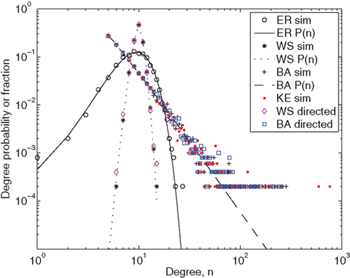
Figure 2. Degree distributions of each undirected network, and out-degree distribution for our directed versions of the Watts and Strogatz (1998) and Barabási and Albert (1999) networks with d = 0.5. Markers show the relative frequency of occurrence of each degree based on a single simulation of each network with size N = 5000. Lines show the mathematical expressions for the degree distribution, P(n), given by Eqns (6), (10), and (14). For the Erdös–Rényi undirected network, and thus p = 0.002. For the Watts–Strogatz undirected network, k_L = 10 and p_w = 0.1. For the Barabási–Albert undirected network, m = m_o = 5. For the Klemm–Eguílez undirected network, μ = 0.1 and m = 5. The same parameters were used for the directed versions of the Watts–Strogatz and Barabási–Albert networks. For the directed networks d = 0.5.

In Figure 2 it is clear that the mathematical expressions for the degree distribution provide an excellent match to the relative frequencies of the occurrences of each degree from even a single simulation of each network. We have chosen N = 5000 as this is sufficiently large for the match to be good. Much smaller N will not produce such a good outcome, but if many independent repeats of each network were produced, and the resulting degree distributions ensemble averaged, we would also expect a good match for smaller N. The scale-free behavior of the Barabási and Albert (1999) and Klemm and Eguílez (2002b) networks is clear from the fact that the degree distribution is approximately a straight line that decreases from small n to large n on the log–log axes of the figure.

Note that for the scale-free networks at large n there is a clear range of values of the degree probabilities that are never achieved. This is simply due to the finite size (N = 5000) of the network and the logarithmic scale of the plot. The smallest degree probabilities shown are at the value 1/5000, which occurs when there is only one node with degree n. The second smallest degree probability is 2/5000, which occurs for nodes with degree two. In general, the degree probabilities are discretized in units of 1/N, and this discretization is most apparent on a logarithmic axis at small probabilities. The deviation of the degree distribution from the straight line predicted for the scale-free networks at this point are also due to the finite size of the network.

In Figure 3, the approximate results for L provide an excellent fit to the data, but the scaling relationships clearly do not align so well for every value of N. This is not due to the fact that we have not averaged over many repeats at each value of N, but because scaling relationships are not approximations in an absolute sense – they instead indicate a general trend (e.g., proportionality) in how one variables changes as another changes. The utility should however be clear, because in this case they illustrate how the average path length is expected to change with network size N, and the simulation data clearly shows the correct qualitative behavior. In all cases, the average path length increases with N, as predicted by the mathematical expressions. Note that we have multiplied each scaling relationship by a constant so that they align with the data points at N = 5000. Other choices, such as a best fit to all data points could also be used.

FIGURE 3

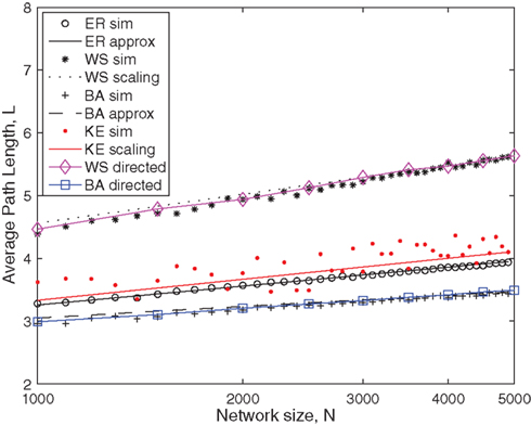
Figure 3. Average path length as a function of network size, N. Markers show results for the average path length based on a single simulation of each network. Lines show the mathematical expressions for the average path length, L, given by Eqns (7), (11), (16), and (18). Note that the scaling relationships have been multiplied by a scalar chosen so that they align with the simulation data points at N = 5000. For the Erdös–Rényi undirected network, and thus p = 10/N. For the Watts–Strogatz undirected network, k_L = 10 and p_w = 0.1. For the Barabási–Albert undirected network, m = m_o = 5. For the Klemm–Eguílez undirected network, μ = 0.1 and m = 5. The same parameters were used for the directed versions of the Watts–Strogatz and Barabási–Albert networks. For the directed networks, d = 0.5.

In Figure 4, there is an excellent match between data for from a single simulation and the mathematical expressions for the Erdös–Rényi and Watts–Strogatz networks. The clustering coefficient for the Barabási–Albert model also clearly decreases with N as suggested by the scaling relationship of Eqn. (17), and slightly more slowly with N than it does for the Erdös–Rényi network, as pointed out by Albert and Barabási (2002). The scaling relationship was fitted in the same way as for Figure 3.

FIGURE 4

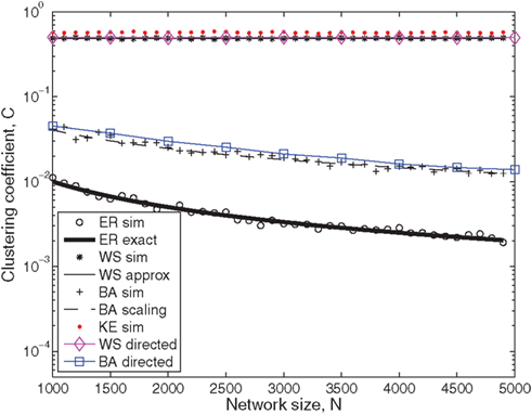
Figure 4. Clustering coefficient as a function of network size, N. Markers show results for the clustering coefficient based on a single simulation of each network. Lines show the mathematical expressions for the clustering coefficient, , given by Eqns (9), (12), and (17). Note that the scaling relationship of (17) was multiplied by a scalar chosen so that it aligns with the simulation data points at N = 5000. For the undirected Erdös–Rényi network, and thus p = 10/N. For the undirected Watts–Strogatz network, k_L = 10 and p_w = 0.1. For the undirected Barabási–Albert network, m = m_o = 5. For the Klemm–Eguílez network, μ = 0.1 and m = 5. The same parameters were used for the directed versions of the Watts–Strogatz and Barabási–Albert networks. For the directed networks, d = 0.5.

The small-world property is evident for the choice of p_w for the Watts–Strogatz network and m for the Klemm–Eguílez network. Although the average path length is larger in the Watts–Strogatz case than it is for an Erdös–Rényi network, it is significantly smaller than the path length for the deterministic lattice generated at the start of the Watts–Strogatz algorithm, which is L = 0.75(k_L − 2)/(k_L − 1) = 2/3. The clustering coefficient for both small-world networks on the other hand, is close to 0.5, which is significantly larger than that of the Erdös–Rényi and Barabási–Albert models. Moreover, the clustering coefficient does not decrease with increasing network size for the Watts–Strogatz and Klemm–Eguílez models, unlike the Erdös–Rényi and Barabási–Albert networks.

Figure 5 demonstrates that the Barabási–Albert network is not small-world in the sense of high clustering. This figure shows the proximity-ratio for the three complex networks, and it is clear that this metric is significantly larger than unity for the Watts–Strogatz and Klemm–Eguílez models, and indeed grows with N for these models, but is relatively small for the Barabási–Albert network, so that according to Walsh (1999), it is not a small-world.

FIGURE 5

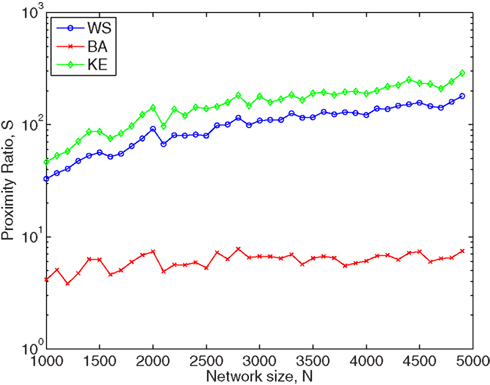
Figure 5. Proximity-ratio for a single simulation of three undirected networks, as a function of network size, N. For the undirected Erdös–Rényi network, and thus p = 10/N. For the undirected Watts–Strogatz network, k_L = 10 and p_w = 0.1. For the undirected Barabási–Albert network, m = m_o = 5. For the undirected Klemm–Eguílez network, μ = 0.1 and m = 5.

Figure 6 replicates the form of Figure 2 from Watts and Strogatz (1998), and Figure 1 from Klemm and Eguílez (2002b) on the same axes, and illustrates how the average path length and clustering coefficient change with p_w and m respectively, relative to p_w = 0 and m = 0. In this case we averaged both statistics over 100 different networks of each type. It is very interesting that the normalized clustering coefficient for the Klemm–Eguílez network follows precisely the same curve as that of the Watts–Strogatz model. The average path length is not the same for the two networks, but both show the characteristic small-world behavior – the average path length rapidly decreases as the probability of randomly reconnecting edges (p_w or m) increases. It is also clear, given the less-smooth average path length curve, that in the Klemm–Eguílez network there is more variance between simulations.

FIGURE 6

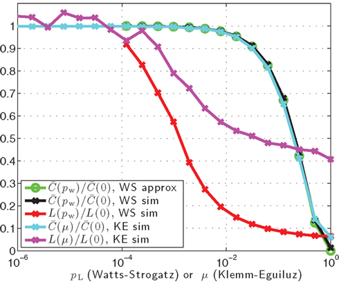
Figure 6. Normalized clustering coefficient and normalized average path length as function of p_w for the Watts and Strogatz (1998) undirected network, with k_L = 10 and N = 1000 and as a function of μ for the Klemm and Eguílez (2002b) network with m = 5 and N = 1000. The normalization is relative to the clustering coefficient and average path length at p_L = 0 or μ = 0, i.e., the case of no random re-wirings in each network. Simulation data is averaged over 100 independently generated networks.

Figures 7–10 show examples that visually illustrate the connectivity amongst each of the four undirected networks. These were created from simulation data using a “force-based” graph method similar to that of Fruchterman and Reingold (1991).

FIGURE 7

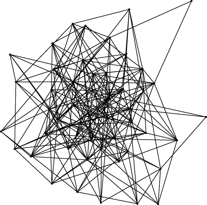
Figure 7. Illustration of the undirected random network generated by the algorithm of Erdös and Rényi (1960) with N = 50 and p = 0.2 (so that ). Nodes with higher degree are placed centrally, and those with lower degree away from the center.

FIGURE 8

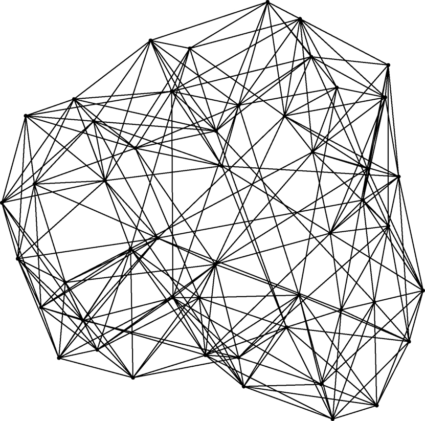
Figure 8. Illustration of the undirected small-world network generated by the algorithm of Watts and Strogatz (1998) with N = 50, p_w = 0.15 and k_L = 10. Nodes with higher degree are placed centrally, and those with lower degree away from the center.

FIGURE 9

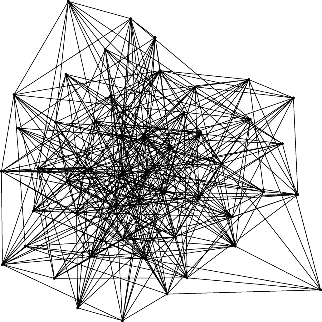
Figure 9. Illustration of the undirected scale-free network generated by the algorithm of Barabási and Albert (1999) with N = 50 and m = m_o = 5 (so that ≃ 10). Nodes with higher degree are placed centrally, and those with lower degree away from the center. Note the small number of high-degree “hubs.”

FIGURE 10

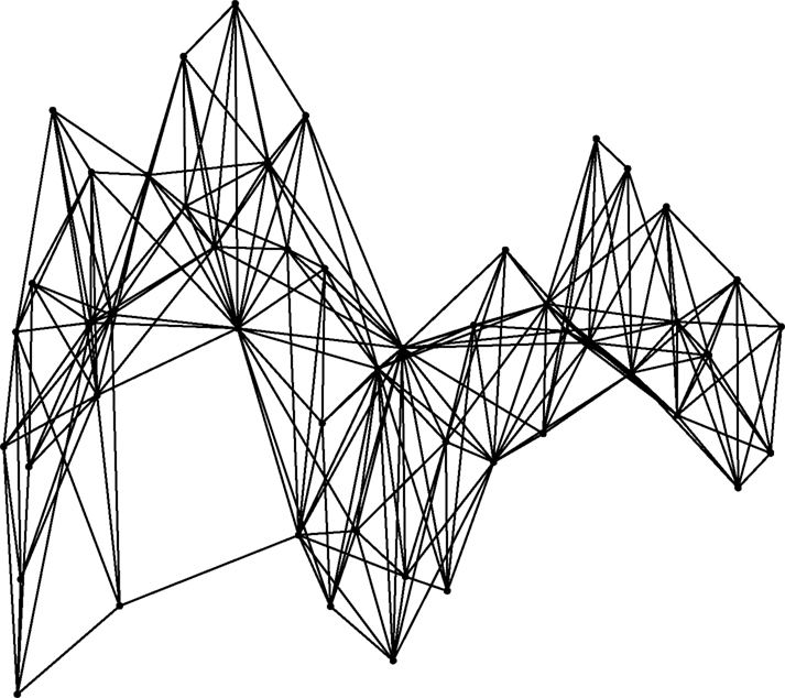
Figure 10. Illustration of the undirected small-world and scale-free network generated by the algorithm of Klemm and Eguílez (2002b), with N = 50, m = 5 (so that ≃ 10) and μ = 0.01. Nodes with higher degree are placed centrally, and those with lower degree away from the center. Note the small number of high-degree “hubs.”

4.2 Directed Networks

Also shown in Figures 2–4 are the out-degree distribution, average path length, and clustering coefficient based on a single simulation for the example directed versions of the Watts–Strogatz and Barabási–Albert models. For these networks we set our parameter d = 0.5, which means that about half the edges are going to/from separate nodes.

There is clearly little difference between the general behavior of the metrics for the undirected and directed versions. Thus, our simulations verify that our directed networks do maintain the same mean in-degree and out-degree as the corresponding undirected network. They also show that with the choice of d = 0.5, that the shown metrics are almost identical to those for the corresponding undirected network.

5 Discussion

5.1 Modular Networks

We mentioned in Section 1.1 that modular networks are a class of network topology of particular relevance to neuroscience. The reasons for this have been recently reviewed by Meunier et al. (2010). Such networks are characterized by identifiable clusters or modules of nodes, within which there are relatively dense numbers of edges. In contrast, the proportion of edges between these modules are relatively low. One characteristic of modular networks, as pointed out by Meunier et al. (2010), is that while they are usually highly clustered small-world networks, not all small-world networks are modular networks.

There is no canonical algorithm for producing modular networks, and we therefore do not describe pseudo-code or simulation results for such networks. Modular networks can however be constructed by adapting other network algorithms for the modules. For example, the modular networks described by Girvan and Newman (2002) can be constructed by adapting the Erdös–Rényi network. Two different edge probabilities, are required: one for edges between nodes within a module, and another for edges between nodes in different modules. The first probability (for an intra-module) is higher, to ensure the network has higher connectivity within the modules than between modules. Another kind of “hierarchical” modular network was described by Ravasz and Barabási (2003).

5.2 Directed Networks

We emphasize that our proposed directed networks are certainly not the only possible way of implementing directed networks with the small-world and scale-free properties. Many algorithms for producing directed networks exist in the literature, e.g., Dorogovtsev et al. (2000) and Klemm and Eguílez (2002a) describe directed scale-free networks based on algorithms very similar to that of Barabási and Albert (1999). The main message is that if the conceptual model is an undirected network, then so should be the simulated model; if it is directed, then the simulation should be directed.

5.3 Tuning Structural Parameters

We mentioned above the tunability of the clustering coefficient and average path length of the Watts and Strogatz (1998) and Klemm and Eguílez (2002b) models. These, of course, are not the only models that can produce tunable characteristics. For example, the model of Bianconi and Barabási (2001) uses a “fitness” model to assign levels of “connectability” to nodes. The distribution function for this factor is used in conjunction with the Barabási and Albert (1999) preferential attachment model to vary the slope of the degree distribution, and thus this more flexible model could be preferable for neuroscience simulations where scale-free degree distributions are required. Similarly, the network of Albert and Barabási (2000) and the directed network introduced by Klemm and Eguílez (2002a) also produces a scale-free degree distribution with an easily tunable slope.

More generally, simple algorithms exist for producing networks with arbitrarily specifiable degree distributions (Molloy and Reed, 1995). Such networks are random in the sense that many different networks with the same degree distribution can exist, and the algorithm produces a single instance from the ensemble of possible networks. See also Newman et al. (2001), who performed comprehensive analysis of generating functions able to produce networks with arbitrary degree distributions, both undirected and directed.

5.4 Other Properties of Networks

Boguñá and Pastor-Satorras (2003) discuss the interesting phenomenon of degree correlation. This is a metric that describes if the respective degrees of two connected nodes are either positively correlated – i.e., assortative mixing, which is usually the case in social networks – or negatively correlated – i.e., disassortative mixing, which is usually the case in technological networks. Boguñá and Pastor-Satorras (2003) go on to generalize the idea of assigning a fitness level to nodes – see e.g., Caldarelli et al. (2000) – to a hidden variable framework, which they use to provide models for the creation of networks with tunable degree correlations and clustering coefficients.

There are many aspects to the study of complex brain networks that we have not discussed here, such as the relationship between structure and function (Bullmore and Sporns, 2009), modeling using weighted networks (Barrat et al., 2004; Rubinov and Sporns, 2010), and the dynamical processes that can occur on networks (Hütt and Lesne, 2009). Moreover, complex networks are not necessarily static, and can vary adaptively and evolve over time (Kozma and Barrat, 2008; Portillo and Gleiser, 2009).

5.5 Comparison of Simulated Networks with Data

Modelers are encouraged to use the networks described in this paper as a starting point, and to adapt them using variations that are informed by specific data. However, this comes with the caveats that (i) it is possible that some dynamical process that takes place within specific networks in the brain may rely on very precise connectivity that a model network that is only statistically similar may be incapable of reproducing; and (ii) that it is not by any means guaranteed that any given algorithm will reproduce precisely all properties, even on average, of experimentally obtained data on the connectivity of neurobiological networks. For example one can produce a graph that is statistically the same in terms of some metrics, but differs in others that are perhaps not relevant to the process being studied.

Simulated networks can however still be useful in studying typical processes within the brain in many ways. For example, if one can identify relevant features, they may be able to ensure their algorithm produces graphs that match these. Another example is that a useful approach to understanding the complex nature of brain networks is to compare metrics produced from empirical data with “null-hypothesis” networks. In this paper we used the proximity-ratio measure of “small-world-ness” – this approach is based on using the Erdös–Rényi G(N, p) network as a “null-hypothesis” network. As pointed out by Sporns (2011), the latter network is by no means the only network that might be specified for the null-hypothesis. A random network with an arbitrary degree distribution but no degree correlations might be generated using the approach of Molloy and Reed (1995) and used as a comparison with an empirical network with the same degree distribution but differences in other metrics.

Conflict of Interest Statement

The authors declare that the research was conducted in the absence of any commercial or financial relationships that could be construed as a potential conflict of interest.

Acknowledgments

Mark D. McDonnell is the recipient of an Australian Research Fellowship funded by the Australian Research Council (project number DP1093425). The authors would like to express gratitude to the referees for many constructive comments and suggestions that improved this manuscript.

References

Achard, S., and Bullmore, E. (2007). Efficiency and cost of economical brain functional networks. PLoS Comput. Biol. 3, e17. doi: 10.1371/journal.pcbi.0030017

Pubmed Abstract | Pubmed Full Text | CrossRef Full Text

Albert, R., and Barabási, A.-L. (2000). Topology of evolving networks: local events and universality. Phys. Rev. Lett. 85, 5234–5237.

Pubmed Abstract | Pubmed Full Text | CrossRef Full Text

Albert, R., and Barabási, A.-L. (2002). Statistical mechanics of complex networks. Rev. Mod. Phys. 74, 47–97.

Barabási, A.-L., and Albert, R. (1999). Emergence of scaling in random networks. Science 286, 509–512

Barabási, A.-L., Albert, R., and Jeong, H. (1999). Mean-field theory for scale-free random networks. Physica A 272, 173–187.

CrossRef Full Text

Barrat, A., Barthelemy, M., Pastor-Satorras, R., and Vespignani, A. (2004). The architecture of complex weighted networks. Proc. Natl. Acad. Sci. U.S.A. 101, 3747–3752.

Pubmed Abstract | Pubmed Full Text

Barrat, A., and Weigt, M. (2000). On the properties of small-world network models. Eur. Phys. J. B 13, 547–560.

Bassett, D. S., and Bullmore, E. (2006). Small-world brain networks. Neuroscientist 12, 512–523.

Pubmed Abstract | Pubmed Full Text | CrossRef Full Text

Bianconi, G., and Barabási, A.-L. (2001). Competition and multiscaling in evolving networks. Europhys. Lett. 54, 436–442.

Boccaletti, S., Latora, V., Moreno, Y., Chavez, M., and Hwang, D.-U. (2006). Complex networks: structure and dynamics. Phys. Rep. 424, 175–308.

CrossRef Full Text

Boguñá, M., and Pastor-Satorras, R. (2003). Class of correlated random networks with hidden variables. Phys. Rev. E 68, 036112.

Bollobás, B., and Riordan, O. (2004). The diameter of a scale-free random graph. Combinatorica 24, 5–34.

CrossRef Full Text

Bullmore, E., and Sporns, O. (2009). Complex brain networks: graph theoretical analysis of structural and functional systems. Nat. Rev. Neurosci. 10, 186–198.

Pubmed Abstract | Pubmed Full Text

Buzsáki, G. (2006). Rhythms of the Brain. Oxford: Oxford University Press.

Caldarelli, G., Marchetti, R., and Pietronero, E. (2000). The fractal properties of internet. Europhys. Lett. 52, 386–391.

Dorogovtsev, S. N., Mendes, J. F. F., and Samukhin, A. N. (2000). Structure of growing networks with preferential linking. Phys. Rev. Lett. 85, 4633–4636.

Pubmed Abstract | Pubmed Full Text | CrossRef Full Text

Erdös, P., and Rényi, A. (1959). On random graphs. Publicationes Mathematica 6, 290–297.

Erdös, P., and Rényi, A. (1960). On the evolution of random graphs. Publ. Math. Inst. Hung. Acad. Sci. 5, 17–61.

Fagiolo, G. (2007). Clustering in complex directed networks. Phys. Rev. E 76, 026107.

Freeman, W. J., and Breakspear, M. (2007). Scale-free neocortical dynamics. Scholarpedia 2, 1357.

Fronczak, A., Fronczak, P., and Holyst, J. A. (2004). Average path length in random networks. Phys. Rev. E 70, 056110.

Fruchterman, T. M. J., and Reingold, E. M. (1991). Graph drawing by force-directed placement. Softw. Pract. Exp. 21, 1129–1164.

Gilbert, E. N. (1959). Random graphs. Ann. Math. Stat. 30, 1141–1144.

Girvan, M., and Newman, M. E. J. (2002). Community structure in social and biological networks. Proc. Natl. Acad. Sci. U.S.A. 99, 7821–7826.

Pubmed Abstract | Pubmed Full Text

He, Y., Chen, Z. J., and Evans, A. C. (2007). Small-world anatomical networks in the human brain revealed by cortical thickness from MRI. Cereb. Cortex 17, 2407–2419.

Pubmed Abstract | Pubmed Full Text

Humphries, M. D., Gurney, K., and Prescott, T. J. (2006). The brainstem reticular formation is a small-world, not scale-free, network. Proc. R. Soc. B 273, 503–511.

Hütt, M.-T., and Lesne, A. (2009). Interplay between topology and dynamics in excitation patterns on hierarchical graphs. Front. Neuroinformatics 3:28. doi: 10.3389/neuro.11.028.2009

Pubmed Abstract | Pubmed Full Text | CrossRef Full Text

Klemm, K., and Eguílez, V. (2002a). Highly clustered scale-free networks. Phys. Rev. E 65, 036123.

CrossRef Full Text

Klemm, K., and Eguílez, V. M. (2002b). Growing scale-free networks with small-world behavior. Phys. Rev. E 65, 57102.

CrossRef Full Text

Kozma, B., and Barrat, A. (2008). Consensus formation on adaptive networks. Phys. Rev. E 77, 016102.

Luce, R., and Perry, A. (1949). A method of matrix analysis of group structure. Psychometrika 14, 95–116.

Pubmed Abstract | Pubmed Full Text | CrossRef Full Text

Meunier, D., Lambiotte, R., and Bullmore, E. T. (2010). Modular and hierarchically modular organization of brain networks. Front. Neurosci. 4: 200. doi: 10.3389/fnins.2010.00200

Pubmed Abstract | Pubmed Full Text | CrossRef Full Text

Milgram, S. (1967). The small world problem. Psychol. Today 2, 60–67.

Molloy, M., and Reed, B. (1995). A critical point for random graphs with a given degree sequence. Random Struct. Algorithms 6, 161–180.

Newman, M., Barabási, A.-L., and Watts, D. J. (2006). The Structure and Dynamics of Networks. Princeton: Princeton University Press.

Newman, M. E. J. (2003). The structure and function of complex networks. SIAM Rev. 45, 167–256.

CrossRef Full Text

Newman, M. E. J., Moore, C., and Watts, D. J. (2000). Mean-field solution of the small-world network model. Phys. Rev. Lett. 84, 3201–3204.

Pubmed Abstract | Pubmed Full Text | CrossRef Full Text

Newman, M. E. J., Strogatz, S. H., and Watts, D. J. (2001). Random graphs with arbitrary degree distributions and their applications. Phys. Rev. E 64, 026118.

Newman, M. E. J., Watts, D. J., and Strogatz, S. H. (2002). Random graph models of social networks. Proc. Natl. Acad. Sci. U.S.A. 99(Suppl. 1), 2566–2572.

Pubmed Abstract | Pubmed Full Text | CrossRef Full Text

Portillo, I. J. G., and Gleiser, P. M. (2009). An adaptive complex network model for brain functional networks. PLoS ONE 4, e6863. doi: 10.1371/journal.pone.0006863

Pubmed Abstract | Pubmed Full Text | CrossRef Full Text

Price, D. J. S. (1965). Networks of scientific papers. Science (New York) 149, 510.

Ravasz, E., and Barabási, A. -L. (2003). Hierarchical organization in complex networks. Phys. Rev. E 67, 026112.

Roxin, A., Riecke, H., and Solla, S. A. (2004). Self-sustained activity in a small-world network of excitable neurons. Phys. Rev. Lett. 92, 198101.

Pubmed Abstract | Pubmed Full Text

Rubinov, M., and Sporns, O. (2010). Complex network measures of brain connectivity: uses and interpretations. Neuroimage 52, 1059–1069.

Pubmed Abstract | Pubmed Full Text | CrossRef Full Text

Schank, T., and Wagner, D. (2005). Approximating clustering coefficient and transitivity. J. Graph Algorithms Appl. 9, 265–275.

Shanahan, M. (2008). Dynamical complexity in small-world networks of spiking neurons. Phys. Rev. E 78, 041924.

Soffer, S. N., and Vázquez, A. (2005). Network clustering coefficient without degree-correlation biases. Phys. Rev. E 71, 057101.

Song, S., Sjöström, P. J., Reigl, M., Nelson, S., and Chklovskii, D. B. (2005). Highly nonrandom features of synaptic connectivity in local cortical circuits. PLoS Biol. 3, e350. doi:10.1371/journal.pbio.0030350

CrossRef Full Text

Sporns, O. (2011). Networks of the Brain. Cambridge, MA: The MIT Press.

Walsh, T. (1999). “Search in a small world,” in Proceedings of the 16th International Joint Conference on Artificial Intelligence, ed. T. Dean (San Francisco, CA: Morgan Kaufmann).

Watts, D. J., and Strogatz, S. H. (1998). Collective dynamics of “small-world” networks. Nature 393, 440–442.

Pubmed Abstract | Pubmed Full Text | CrossRef Full Text