Clustering predicts memory performance in networks of spiking and non-spiking neurons

Introduction

Network models for associative memories store the information to be retrieved in the values of the synaptic weights. Weighted summation of their synaptic inputs then allows the neurons to transform any input pattern into an associated output pattern. Network models for associative memories come in two flavors. In pure feedforward models, like the one-layer perceptron, a static input pattern in the afferent fibers is in one step transformed, by weighted summation, into a static pattern of activity of the neurons in the output layer. For instance Purkinje cells in the cerebellum have been proposed to recognize in this way patterns of activity in the mossy fibers (Marr, 1969; Tyrrell and Willshaw, 1992; Steuber et al., 2007). In feedback models, which are the subject of the present paper, the memory is stored in the weights of recurrent connections between the neurons. The input pattern (one input for each neuron) initializes the neurons, after which the network is left free to run until the neuronal activities potentially converge to a stable pattern, which no longer changes over time. The main advantage of feedback networks is that they can work self-correctively: noisy input patterns can converge to the original attractor pattern. The main questions are how a desired memory can be stored by making it an attractor of the network (the learning rule determining the synaptic weights) and how many patterns can be stored and retrieved, within a given error margin, in a network with a given number of neurons and synapses.

These questions were solved analytically for the so-called Hopfield network (Hopfield, 1982), which, however, takes several simplifications that are biologically unrealistic. The Hopfield network, in its original formulation, consists of two-state (bipolar) neurons that are fully connected to each other, with each pair connected bi-directionally with identical weights. More biologically realistic adaptations of the Hopfield network, using sparse and non-symmetrical connections, have been shown to have, like the perceptron, a capacity of 2k patterns, k being the number of connections to each neuron (Diederich and Opper, 1987; Gardner, 1988).

In the present paper, building on our previous work (Davey and Adams, 2004; Calcraft et al., 2006, 2007, 2008; Davey et al., 2006; Chen et al., 2009), we use computer simulations to address three other biological constraints for sparsely connected networks. Firstly, how does the topology of the wiring pattern affect memory performance? Secondly, can memories be retrieved by a network of spiking neurons with connection delays? Thirdly, taking into account wiring length, which wiring pattern has the highest cost efficiency?

Materials and Methods

The Network Model for Associative Memory

Network connectivity

For each model investigated, a collection of N artificial neurons is placed on a line such that the nodes are equally spaced. To avoid edge effects we consider the ends of the line to meet, so that we have a so-called periodic boundary. This gives the network a ring topology. For simplicity we define the distance between neighboring neurons to be 1. To aid in visualization we represent the networks as a ring, but they are always actually 1-D. Once the neurons have been positioned they can be connected to one another in a variety of fashions. However, there are three common features shared among all network models. Firstly, the networks are regular, so that each neuron has k incoming connections. To maintain this fan-in during rewiring, only the index of the source (afferent) neuron of a connection could be changed. Therefore although the connection strategy varies in the present study, the values of N and k are constant. Secondly, the networks are sparse, so that with a network of N units, k ≪ N, resembling the sparse connectivity of the mammalian cortex. Thirdly, the connections are directed, so if the connection from i to j exists, this does not imply that the reciprocal connection from j to i also exists.

With this configuration, two extreme cases are widely known and commonly studied. The first case is a completely local network, or lattice, whose nodes are connected to those nodes that are closest to it. An example of a local network is the cellular neural network (CNN), where units are connected locally in 2-D (Brucoli et al., 1996). Alternatively the network can be connected in a completely random manner, where the probability of any two nodes being connected is k/N, independently of their position. Locally connected networks have a minimum wiring length, but perform poorly as associative memories, since pattern correction is a global computation and full local connectivity does not allow easy passage of information across the whole network. In randomly connected networks, on the other hand, information can readily move through the network, and consequently pattern correction is much better and in fact cannot be improved with any other architecture. However, in real biological networks such as cerebral cortex, completely random connectivity suffers from the restriction of high wiring cost and therefore may not be the desirable choice. An optimized connectivity is one that gives a performance comparable to random networks, but with more economical wiring. The existence of such connectivity, as well as its construction strategy, has been of great interest in recent research. One family of network connectivities, the so-called small-world networks (Watts and Strogatz, 1998), has been suggested to exhibit this optimization.

Our first connection strategy is adapted from the method proposed by Watts and Strogatz (1998). The Watts–Strogatz small-world network starts from a local network, where each unit has incoming connections from its k nearest neighbors (to simplify results, networks studied in this paper have no self-connectivity). The local network is then progressively rewired by randomly re-assigning a fraction (p) of the afferent neurons. The network is transformed into a completely random network when p reaches 1 (Figure 1). In the rest of the paper we refer to networks constructed in this way as small-world networks.

FIGURE 1

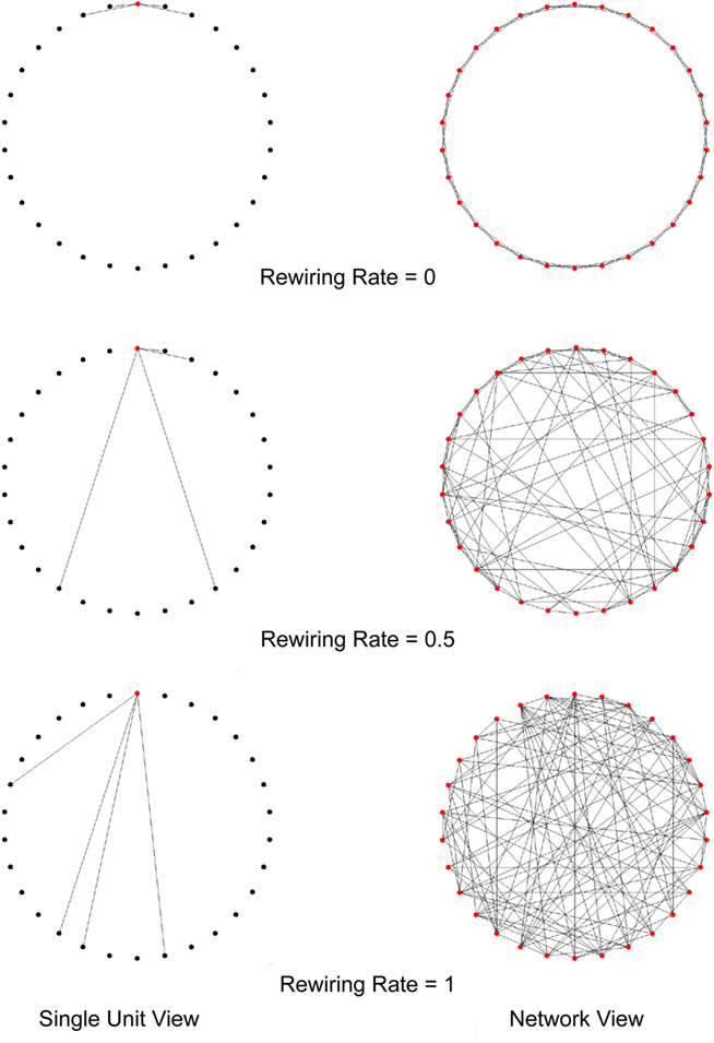
Figure 1. The rewiring process in a Watts–Strogatz small-world network. In this example, the network contains 30 units and four afferent connections to each unit. Initially all units are locally connected, as p = 0. Then a proportion of connections of each unit are randomly rewired (p = 0.5). As the rewiring rate increases, the network becomes a completely random network (p = 1). Note that the connections are formed on a one dimensional line but are drawn in 2-D figures for better visualization.

Another connection strategy investigated by us exhibits Gaussian connectivity, where each unit has k incoming connections from neurons whose distances form a Gaussian distribution (see Figure 7). The connectivity of such a network is parameterized by the SD of its distance distribution, σ. We have shown in earlier work (Calcraft et al., 2007) that both small-world and Gaussian networks can perform optimally as associative memories and that tight Gaussian distributions give very parsimonious networks with efficient use of connecting fiber.

The biological context of this connectivity comes from the mammalian cortex, which is thought to have a similar connectivity between individual neurons (Hellwig, 2000).

The modularity of mammalian cortex, commonly referred to as the hypothesis of cortical columns (Mountcastle, 1997), is also considered in our investigation. Three different types of modular connectivity are studied. The first one, named the Fully Connected Modular network, contains m internally fully connected subnetworks, defined as modules. Initially there is no interconnection between modules, thus each module can be treated as an isolated fully connected associative memory model. The subnetworks establish connections by randomly rewiring the intra-modular connections to form random connections from anywhere across the whole network. A fraction p denotes the proportion of rewired connections. The network has the same type of connectivity as the Watts–Strogatz small-world network, when p reaches 1. Figure 2 gives an example of networks with this connectivity.

FIGURE 2

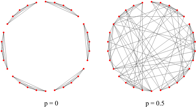
Figure 2. The construction of a Fully Connected Modular network. Each network has 30 units and four afferent connections to each unit. The network is initialized as six discrete modules with fully connected internal networks (left, with rewiring rate p = 0). To connect these modules, internal connections are then rewired randomly across the whole network (right, with rewiring rate p = 0.5). Note that the regularity of the network is maintained during the rewiring (each node always has four afferent connections).

Another modular network we have investigated is called the Gaussian-Uniform Modular Network. In such a network, the intra-modular connections within each module have a Gaussian-distributed connectivity with a SD of σ_internal, which is proportional to the number of internal connections per unit, k_internal. Each unit in the network also has a number of external connections (defined by k_external) from units in other modules. The connectivity of the external network is uniformly random. Although k_internal and k_external vary in different configurations, the total number of connections per unit, k = k_internal + k_internal, is maintained so that the performances of different networks can be compared.

The neuron model, learning, and dynamics

The best connection strategy for an associative memory network may be dependent on details of the neuron model. For instance, the wiring length of a connection may have no significant impact on simple threshold neuron models, but is important in a spiking model simulating geometry-dependent time delays. To reveal the intrinsic principles that may govern network construction, this paper investigates connection strategies in various associative memory networks with either the traditional threshold unit models or the more biologically realistic, leaky integrate-and-fire spiking neuron models.

Each model needs to be trained before any measure of performance can be obtained. Canonical associative memory models with threshold units, for example the Hopfield net, commonly use a one-shot Hebbian learning rule. This, however, does not perform well if the networks are sparse and non-symmetric (Davey et al., 2006). In this paper, we adapt a more useful approach using standard perceptron learning.

A set of random, bipolar, or binary vectors is presented as training patterns, where the probability of any bit on the pattern being on (+1), referred to as the bias of the pattern, is 0.5. The patterns can be learned by the following learning rule:

Begin with zero weights
Repeat until all units are correct
    Set state of network to one of the training
    pattern ξp
    For each unit, i, in turn:
          Calculate its net input, .
          If or
          then change all the weights to unit i
          according to:
                 when
                 when

The value denotes the ith bit of pattern p being +1, and the value denotes the value −1 or 0 according to the type of network. Network performance improves till saturation when the learning threshold T increases, irrespective of the value of k. However, increasing T also means a longer training time, and the improvement is insignificant for very high values of T. Here we set T = 10, based on results from our previous study (Davey and Adams, 2004).

For threshold unit models we use the standard bipolar +1/−1 representation. For the spiking networks we use 1/0 binary patterns, as they can be easily mapped onto the presence or absence of spikes.

Threshold unit models and integrate-and-fire spiking neuron models require different update dynamics. For threshold unit models, we use the standard asynchronous dynamics: units output +1 if their net input is positive and −1 if negative. As the connectivity is not symmetrical there is no guarantee that the network will converge to a fixed point, but, in practice these networks normally exhibit straightforward dynamics (Davey and Adams, 2004) and converge within hundreds of epochs (one epoch is a full update of every unit in the network in a fixed order). We arbitrarily set a hard limit of 5000 epochs, at which we take the network state as final even if it may not be at a fixed point. Networks with spiking neurons, on the other hand, were numerically integrated, and their state was evaluated after 500 ms (see below).

Due to the intrinsic model complexity, associative memory models with spiking units require careful tuning so that the performance is comparable to threshold unit models. We use a leaky integrate-and-fire neuron model which includes synaptic integration, conduction delays, and external current charges. The membrane potential V of each neuron in the network is set to a resting membrane potential of 0 mV if no stimulation is presented. The neuron can be stimulated and change its potential by either receiving spikes from other connected neurons, or by receiving externally applied current. If the membrane potential of a neuron reaches a fixed firing threshold, T_firing, which is set to 20 mV, the neuron emits a spike and the potential is reset to the resting state (0 mV) for a certain period (the refractory period, set to 3 ms). During this period the neuron cannot fire another spike even if it receives very strong stimulation.

A spike that arrives at a synapse triggers a current; the density of this current (in A/F), I_ij(t), is given by

where i refers to the postsynaptic neuron and j to the presynaptic neuron. τ_s = 2 ms is the synaptic time constant, t_spike is the time when the spike is emitted by neuron j, and t_spike + delay_ij defines the time when the spike arrives at neuron j. Two delay modes were implemented in our study. The fixed-delay mode gives each connection a fixed 1 ms delay. In the second mode, the delay of spikes in a connection is defined by

where d_ij is the connection distance which is defined as the minimum number of steps between neuron i and j along the ring, since the distance between neighboring neurons is 1, as described in Section “The Network Model for Associative Memory.” The formula is a rough mapping from a one dimensional structure to a realistic 3-D system.

The change of membrane potential is defined by

In this equation, −(V/τ_m) is the leak current density, while τ_m = 50 ms is the membrane time constant. I_external is the external current density which will be discussed later. The internal current is summed by Σ_{i ≠ j ∈ G}C_ijI_ijW_ij where C_ij = 1 indicates the presence of a connection from j to i, and C_ij = 0 otherwise. W_ij is the weight of the connection from neuron j to i trained by the above learning rule.

In networks trained with a learning threshold T = 10, a single spike from an excitatory (positive-weight) connection generates a postsynaptic potential (EPSP) of about 3 ∼ 4 mV on average, and inhibitory (negative-weight) connections generate similar voltage deflections of negative sign (IPSPs). Since the proportion of excitatory and inhibitory connections is balanced (the network is trained with unbiased patterns), it requires the excess of six to seven spikes at excitatory connections to trigger the firing of a unit. Scaling down the connection weights to reduce the EPSPs also reduces the IPSPs proportionally, resulting in little or no improvement on the network’s associative memory performance. The whole network is silenced, however, when all weights are scaled down to less than 20% of their original trained values, due to the current leak in the neuron model.

External currents are injected into the network in order to trigger the first spikes in the simulation. Each current injection transforms a static binary pattern to a set of current densities. Given an input pattern, unit i receives an external current if it is on in that pattern, otherwise the unit receives no external current. An external current has a density of 3A/F and is continually applied to the unit for the first 50 ms of simulation. This mechanism guarantees that the first spiking pattern triggered in the network reflects the structure of the input pattern. After the first spikes (about 7–8 ms from the start of a simulation), both internal currents caused by spikes, and the external currents, affect the network dynamics. Spike activity continues after the removal of external currents, as the internal currents caused by spike trains become the driving force. The network is then allowed to run for 500 ms, after which time the network activity has stabilized, before its spiking pattern is evaluated.

Measures of Memory Performance

The associative memory performance of the threshold unit network is measured by its effective capacity (EC; Calcraft, 2005). EC is a measure of the maximum number of patterns that can be stored in the network with reasonable pattern correction still taking place. In other words, it is a capacity measure that takes into account the dynamic ability of the network to perform pattern correction. We take a fairly arbitrary definition of reasonable as the ability to correct the addition of 60% noise (redrawing 60% of the pattern bits) to within a similarity of 95% with the original fundamental memory, that is, 95% of the bits are identical. Varying these 2% figures gives differing values for EC but the values with these settings are robust for comparison purposes. For large fully connected networks the EC value is about 0.1 of the conventional capacity of the network, but for networks with sparse, structured connectivity EC is dependent upon the actual connectivity pattern.

The EC of a particular network is determined as follows:

Initialize the number of patterns, P, to 0
Repeat
      Increment P
      Create a training set of P random patterns
      Train the network
      For each pattern in the training set
          Degrade the pattern randomly by adding 60% of noise
          With this noisy pattern as start state, allow the network to converge
          Calculate the similarity of the final network state with the original pattern
      EndFor
      Calculate the mean pattern similarity over all final states
      until the mean pattern similarity is less than 95%
The Effective Capacity is then P-1.

The EC of the network is therefore the highest pattern loading for which a 60% corrupted pattern has, after convergence, a mean similarity of 95%, or greater with its original value.

The EC measure needs modification to suit the spiking model. We adopt the concept of memory retrieval from Anishchenko and Treves (2006). For p training patterns, the memory retrieval, M, is defined by

O^μ(t) is the overlap of the network activity and pattern μ at time t, more particularly the cosine of the angle between both vectors,

where r_i(t) is the number of spikes emitted by unit i during a time window [t − t_w, t] (we use a window of 10 ms). is the chance level of overlap with other patterns when the external currents are injected to the network based on pattern μ

The memory retrieval measure was designed for sparse patterns where the chance overlap is important. In our case the patterns are unbiased so the chance overlap is close to 0. The memory retrieval M ranges between 1 and −1, in which a high value indicates better performance. The 95% pattern similarity in the threshold unit model corresponds to a 0.9 memory retrieval value M in the spiking neuron model, thus we use these two values as the EC criteria in this investigation.

Connectivity Measures

In recent years connectivity measures from Graph Theory have been used in the investigation of both biological and artificial neural networks. We use two of these measures to quantify our connectivity strategies.

A common measure of network connectivity is Mean Path Length. The Mean Path Length of a network G, L(G), is defined as:

where p_ij is the length of the shortest connecting path from unit j to unit i. It is important to note here that the length of a path in the graph G is the number of edges that make up the path – it has no relation to the physical distance between the nodes, d_ij.

The Mean Path Length was originally used to define the “small-world” phenomenon found in social science (Milgram, 1967). This refers to the idea that, if a person is one step away from each person they know and two steps away from each person who is known by one of the people they know, then everyone is an average of six steps away from each person in a region like North America. Hence everyone is fairly closely related to everyone else giving a “small-world.”

A fully connected network has the shortest and unique Mean Path Length of 1, whilst in sparse networks the measure varies for different types of connectivity (see Tables in Appendix). A locally connected network has a high Mean Path Length, since each unit is only connected to its nearest neighbors and it is difficult to reach distal units. On the other hand, completely random networks usually have short Mean Path Lengths. Intermediate cases, for example the Watts–Strogatz small-world network, have Mean Path Lengths similar to completely random networks, but significantly lower than the ones of lattices.

Although commonly used as a connectivity measure of neural networks, our investigation reveals that the Mean Path Length is insensitive to connectivity changes if the network is far from local. Another measure, named the Clustering Coefficient, is found to be more sensitive to connectivity changes, and exhibits a good correlation with the associative memory performance.

The definition of Clustering Coefficient is as follows. First we define neighbors of a node in a graph as its directly connected nodes.

Then we define G_i as the subgraph of the neighbors of node i (excluding i itself). C_i, the local Clustering Coefficient of node i, is defined as:

which denotes the fraction of all possible edges of G_i which exist. The Clustering Coefficient of the graph G, C(G), is then defined as the average of c_i, over all nodes of G:

The Clustering Coefficient of a fully connected network is 1, since each node is connected to all others directly. Locally connected sparse networks have high Clustering Coefficients whilst in a completely random networks it is usually low. Interestingly, the so-called small-world networks usually have high Clustering Coefficients, similar to local networks, but short Mean Path Lengths, like completely random networks. Such types of connectivity (short Mean Path Length, high Clustering Coefficient) are also observed in natural networks, for instance, the mammalian cortex.

Results

All networks in our study have 5000 units. The first set of results are for the non-spiking model with 250 incoming connections per unit, that is, N = 5000 and k = 250. The theoretical maximum capacity of such a network with threshold units is known to be 2k = 500 for unbiased random patterns, although in practice the capacity reduces due to pattern correlations. As mentioned in Section “The Neuron Model, Learning, and Dynamics,” we set the learning threshold at T = 10 and the maximum number of updating epochs at 5000. For each network connectivity, results are averages over 10 runs. Errors bars are too small to be visible and therefore are omitted from the figures. The characteristics of different networks and their EC performances are tabulated in Section “Appendix.” The first column of each table contains the values of the independent variable that was varied to construct different networks with the same connection strategy.

Path Length as a Predictor of Performance

As pattern correction is a global computation intuitively one might expect networks with shorter mean path lengths to perform better than those with longer mean path lengths. Our results, shown in Figure 3A to some extent confirm this. The two networks with only local connections (to the right of the graph) and thereby long path lengths, do perform poorly. However path length does not discriminate amongst the majority of network architectures. This is mainly due to the fact that mean path length saturates very quickly once a few long-range connections, which act as global shortcuts, are introduced to a local network. The Tables in Section “Appendix” show that almost all the networks examined here have very similar mean path lengths of around two steps, in spite of the great variation of the independent variables.

FIGURE 3

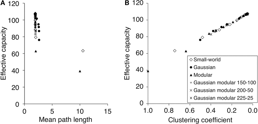
Figure 3. Connectivity measures and memory performance of non-spiking network models. (A) Effective Capacity against Mean Path Length for Watts–Strogatz small-world (with varying amounts of rewiring), Gaussian-Distributed and Fully Connected Modular connectivity strategies. The two local networks have a significantly higher Mean Path Length of about 10, whilst Mean Path Lengths for all other networks are low and do not vary greatly. (B) Effective Capacity against Clustering Coefficient for a variety of networks. Number labels of different series indicate the k_internal − k_external configuration of that network series. The correlation is highly similar and linear for different types of connectivity.

Clustering Coefficient as a Predictor of Performance

Once again intuition suggests that performance could be related to clustering. In a highly clustered network global computation could be difficult: with information staying within clustered subnetworks and not passing through the whole network. This is confirmed by our results in Figure 3B. The networks plotted on the left side of the graph, which are highly clustered, show poor performance. But perhaps what is most noticeable about these results is the obvious linear correlation between the clustering coefficient and performance. So the clustering of a network, regardless of the details of its architecture (small-world, modular, Gaussian) completely predicts its ability to perform as an effective associative memory. A purely static property of the connection matrix appears to determine the ability of a sparsely connected recurrent neural network to perform pattern completion. We will return to why this might be the case in the discussion.

The Integrate-and-Fire Network Model

We now examine how well our results generalize to the more complicated integrate-and-fire model. Because the EC evaluation of this network takes much longer to compute than for the threshold unit model, we reduced the number of incoming connections per unit, k, to 100. For the same reason, only the Watts–Strogatz Small-World network, the Gaussian network, and the Fully Connected Modular network were simulated using integrate-and-fire models. It is interesting to study whether the non-spiking network provides a qualitative and/or quantitative prediction of the much more complex spiking model. Figure 4 compares the performance of three different types of dynamics: non-spiking, spiking with fixed-delay, and spiking with distance-dependent delays. The comparison is illustrated for Gaussian connectivity patterns. Similar comparisons can be made for other connection strategies from the data given in Section “Appendix.” The connectivity of the networks furthest to the left has a very tight Gaussian distribution (σ = 0.4). Interestingly all three networks give a similar EC value of about 25. In all three networks performance then improves as some distal connections are introduced, until the non-spiking network attains its best performance of EC = 42. However the spiking networks show further improvements reaching EC values of over 50. But perhaps the most striking feature of this result is that the simple threshold model provides a good approximation of the much more complex spiking neural network.

FIGURE 4

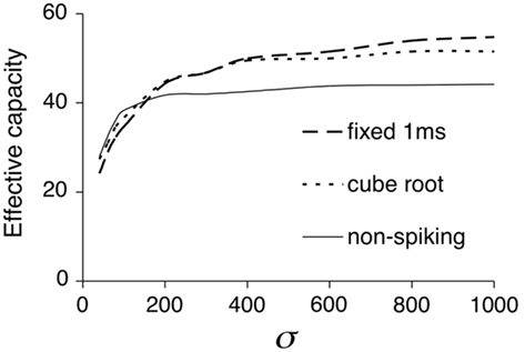
Figure 4. A comparison of the non-spiking network and two versions of the spiking network. All networks have Gaussian connectivity with varying σ. The differences between the three types of the network for large σ are significant. Results for other networks can be found in Section “Appendix.”

Figure 5 presents the results of EC against Clustering Coefficient for spiking models with fixed time delay (1 ms) and cube-root delay. The linear correlation between EC and Clustering Coefficient is not absolutely maintained in the spiking models, however the results still show that the EC increases as the Clustering Coefficient decreases. In the fixed-delay models, the performance of all three patterns of connectivity is very similar, whilst in the cube-root delay models, the performance of the Gaussian connectivity varies more linearly than that of the other two connectivities. This is because the other two types of connectivity have more distal connections due to their uniform rewiring, consequently increasing the distance-dependent delay of the networks. Overall the Clustering Coefficient can still be used as a reasonable predictor of associative memory performance.

FIGURE 5

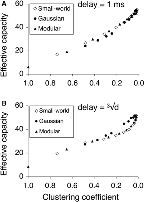
Figure 5. Correlation between Effective Capacity and Clustering Coefficient for spiking network models. For detailed results see Section “Appendix.” (A) Fixed 1 ms delay spiking associative memory models with different connectivity. (B) Cube-root distance delay.

Connection Strategies for Optimizing Wiring Cost and Performance

In nature, the construction of associative memory networks is restricted by resource, thus a connection strategy that optimizes both wiring cost and performance would be preferable. We define the wiring cost of two connected nodes in the network simply as the distance between them, and average it over all connected nodes in the network. Note that this is a quite different measure to mean path length, which measures steps along the connection graph. This measure is also different from the connection delay used in the spiking network models, where the cube-root of d was taken to avoid unrealistically long delays. For simplicity this section focuses on the performance of the threshold unit models.

Figure 6 plots the EC against the Mean Wiring Cost for different connectivity patterns. The Gaussian-distributed network has the most efficient connectivity, that is, for a given mean wiring cost, it has the highest EC. The fully connected Modular network is the least efficient one, whilst the Watts–Strogatz small-world network, and Gaussian-uniform Modular network lay between them. Effective Gaussian networks can be constructed with very low wiring cost because the width of the distribution can be quite small. In fact a width of just 2k (here 500) gives good performance at low cost. We also found that the distribution does not need to increase in width as the network gets bigger (Calcraft et al., 2007).

FIGURE 6

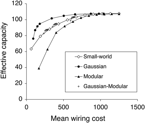
Figure 6. Effective Capacity against Mean Wiring Cost for different connectivity strategies. The best networks occupy the top left of the graph. The Gaussian-Distributed network is the most efficient connectivity among those investigated connectivity, whilst the Fully Connected Modular network is the least efficient one.

Discussion

Our study of memory performance in networks with varying connection strategies extends previous work on the effect of connectivity on network dynamics (Stewart, 2004; Percha et al., 2005), wiring economy and development (Chklovskii et al., 2004), and disease (Belmonte et al., 2004; Lynall et al., 2010; Stam, 2010).

Main Findings and Limitations

The main finding of the present study is that for networks with a fixed number k of connections, and hence a theoretical maximum storage capacity of 2k random patterns, the degree of clustering can be regarded as a negative predictor of memory performance. This prediction is independent of the connection rule used. We further demonstrated that when the cost of wiring is taken into account, by penalizing long-range connections, networks with local Gaussian-distributed connections perform best, and even outperform small-world networks. Finally, these findings also hold when memory is stored and retrieved in networks of spiking neurons with connection delays.

These results were obtained with random uncorrelated patterns, hence without taking into account the statistics of a natural environment. The patterns were stationary (no sequences) and so was largely the dynamics of the network (no oscillations or temporal patterns). Our study was conducted on a ring of neurons, but the results can be extended to 2-D networks (Calcraft et al., 2008).

In the network of spiking neurons, the resulting feedback excitation and inhibition forced the neurons into persistent UP or DOWN states. The network lacked, however, dynamical behavior like gain control, synchronization, or rhythm generation, for which separate populations of excitatory and inhibitory neurons would be required (Sommer and Wennekers, 2001; de Almeida et al., 2007). In addition, the spiking network used the same synaptic weights as obtained with the perceptron-rule for bipolar neurons, and was only tested for memory retrieval. Learning in such networks would require a more advanced algorithm like spike-timing-dependent plasticity.

Clustering as a Negative Predictor of Memory Performance

Clustering (the occurrence of connections between the targets of the same neuron) may make some connections functionally redundant or induce loops. Cycling through loops may hamper convergence to an attractor. In addition, Zhang and Chen (2008) formally demonstrated that loops also induce correlations between states, or equivalently, they induce noise in the form of an interpattern crosstalk term to a neuron’s input, and hence affect pattern separation. Note that this does not directly imply that inducing clustering by adding local connections would worsen memory performance, since the added connections would increment k and hence the maximum capacity as well.

Memory Storage with Local Connectivity

An unexpected finding was that for a given wiring cost, Gaussian-connected networks performed better than small-world networks. Although very-long-range connections speed up the convergence to an attractor during memory retrieval (Calcraft et al., 2007), they do not enhance the steady-state performance of the network. Moreover, the width (SD) of the Gaussian connection kernel can be small (Figure 4), and does not scale with network size.

Relation to Brain Connectivity

The connectivity of the brain, and more particularly of neocortex, is sparse, but certainly not random (see Laughlin and Sejnowski, 2003). Counting the close appositions between axonal and dendritic trees of reconstructed pyramidal cells assembled in a computer network, Hellwig (2000) estimated that connection probability decreased with inter-neuron distance as a Gaussian function of about 500 μm width (the order of magnitude of a cortical column; see Figure 7). Recent experiments using distant release of caged glutamate by photo-stimulation extend this range, indicating a still considerable excitation from distances up to 2 mm (Schnepel et al., 2010).

FIGURE 7

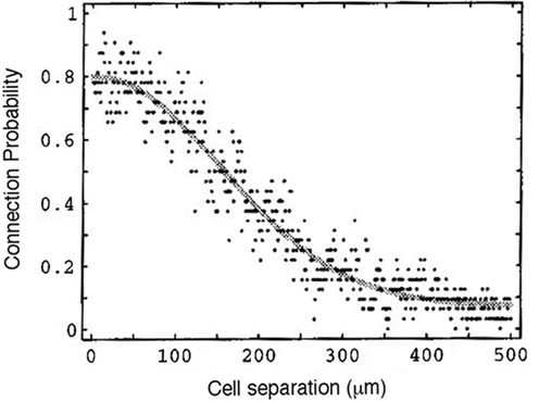
Figure 7. Estimated connection probability between two layer-3 pyramidal neurons of rat visual cortex. Copied from Hellwig (2000) with permission of Springer-Verlag. The best-fitting Gaussian has a SD of 296.7 μm.

Within a column, Song et al. (2005) found an overrepresentation of bi-directional connections and local three-neuron clusters in rat visual cortex. Whereas such clustering may be a sign of a genuine small-world connectivity, the observed clustering of connections may also have a function in the dynamics of the network, or be a consequence of the multidimensional representation of the visual field onto neocortex, mapping not only stimulus position but also higher-order stimulus attributes like orientation. Nevertheless, neocortex is assumed to have a small, but significant, small-worldness (Gerhard et al., 2010), as based on a metric using the ratio of clustering over relative path length (Humphries and Gurney, 2008).

Conclusion

We studied the capacity of memory storage and retrieval in networks of bipolar and spiking neurons, and compared different connection strategies and connection metrics. The single metric best predicting memory performance, for all strategies, was the clustering coefficient, with performance being highest when clustering was low. In large networks, the best connection strategy was a local Gaussian probability function of distance, both in terms of avoiding clustering and of minimizing the cost of wiring.

Conflict of Interest Statement

The authors declare that the research was conducted in the absence of any commercial or financial relationships that could be construed as a potential conflict of interest.

References

Anishchenko, A., and Treves, A. (2006). Autoassociative memory retrieval and spontaneous activity bumps in small-world networks of integrate-and-fire neurons. J. Physiol. (Paris) 100, 225–236.

Pubmed Abstract | Pubmed Full Text | CrossRef Full Text

Belmonte, M. K., Allen, G., Beckel-Mitchener, A., Boulanger, L. M., Carper, R. A., and Webb, S. J. (2004). Autism and abnormal development of brain connectivity. J. Neurosci. 24, 9228–9231.

Pubmed Abstract | Pubmed Full Text | CrossRef Full Text

Brucoli, M., Carnimeo, L., and Grassi, G. (1996). “Implementation of cellular neural networks for heteroassociative and autoassociative memories,” Proceedings of the Fourth IEEE International Workshop on Cellular Neural Networks and their Applications 1996, Seville, 63–68.

CrossRef Full Text

Calcraft, L. (2005). “Measuring the performance of associative memories,” in Computer Science Technical Report 420, University of Hertfordshire, Hatfield, Herts.

Calcraft, L., Adams, R., and Davey, N. (2006). Locally-connected and small-world associative memories in large networks. Neural Inf. Process. Lett. Rev. 10, 19–26.

Calcraft, L., Adams, R., and Davey, N. (2007). Efficient architectures for sparsely-connected high capacity associative memory models. Conn. Sci. 19, 163–175.

Calcraft, L., Adams, R., and Davey, N. (2008). Efficient connection strategies in 1D and 2D associative memory models with and without displaced connectivity. Biosystems 94, 87–94.

Pubmed Abstract | Pubmed Full Text | CrossRef Full Text

Chen, W., Maex, R., Adams, R., Steuber, V., Calcraft, L., and Davey, N. (2009). “Connection strategies in associative memory models with spiking and non-spiking neurons,” in Adaptive and Natural Computing Algorithms, eds M. Kolehmainen, P. Toivanen, and B. Beliczynski (Berlin: Springer Verlag), 42–51. [Lecture Notes in Computer Science 5495].

Chklovskii, D. B., Mel, B. W., and Svoboda, K. (2004). Cortical rewiring and information storage. Nature 431, 782–788.

Pubmed Abstract | Pubmed Full Text | CrossRef Full Text

Davey, N., and Adams, R. (2004). High capacity associative memories and connection constraints. Conn. Sci. 16, 47–66.

Davey, N., Calcraft, L., and Adams, R. (2006). High capacity, small world associative memory models. Conn. Sci. 18, 247–264.

de Almeida, L., Idiart, M., and Lisman, J. E. (2007). Memory retrieval time and memory capacity of the CA3 network: role of gamma frequency oscillations. Learn. Mem. 14, 795–806.

Pubmed Abstract | Pubmed Full Text

Diederich, S., and Opper, M. (1987). Learning of correlated patterns in spin-glass networks by local learning rules. Phys. Rev. Lett. 58, 949–952.

Pubmed Abstract | Pubmed Full Text | CrossRef Full Text

Gardner, E. (1988). The space of interactions in neural network models. J. Phys. A 21, 257–270.

Gerhard, F., Pipa, G., and Gerstner, W. (2010). Estimating small-world topology of neural networks from multi-electrode recordings. Front. Comput. Neurosci. doi: 10.3389/conf.fncom.2010.51.00088.

CrossRef Full Text

Hellwig, B. (2000). A quantitative analysis of the local connectivity between pyramidal neurons in layers 2/3 of the rat visual cortex. Biol. Cybern. 82, 111–121.

Pubmed Abstract | Pubmed Full Text | CrossRef Full Text

Hopfield, J. J. (1982). Neural networks and physical systems with emergent collective computational abilities. Proc. Natl. Acad. Sci. U.S.A. 79, 2554–2558.

Pubmed Abstract | Pubmed Full Text

Humphries, M. D., and Gurney, K. (2008). Network “small-world-ness”: a quantitative method for determining canonical network equivalence. PLoS ONE 3, e0002051. doi: 10.1371/journal.pone.0002051

Pubmed Abstract | Pubmed Full Text | CrossRef Full Text

Laughlin, S. B., and Sejnowski, T. J. (2003). Communication in neuronal networks. Science 301, 1870–1874.

Pubmed Abstract | Pubmed Full Text | CrossRef Full Text

Lynall, M. E., Bassett, D. S., Kerwin, R., McKenna, P. J., Kitzbichler, M., Muller, U., and Bullmore, E. (2010). Functional connectivity and brain networks in schizophrenia. J. Neurosci. 30, 9477–9487.

Pubmed Abstract | Pubmed Full Text

Marr, D. (1969). A theory of cerebellar cortex. J. Physiol. 202, 437–470.

Pubmed Abstract | Pubmed Full Text

Milgram, S. (1967). The Small World Problem. Psychol. Today 1, 60–67.

Mountcastle, V. B. (1997). The columnar organization of the neocortex. Brain 120, 701–722.

Pubmed Abstract | Pubmed Full Text | CrossRef Full Text

Percha, B., Dzakpasu, R., Zochowski, M., and Parent, J. (2005). Transition from local to global phase synchrony in small world neural network and its possible implications for epilepsy. Phys. Rev. E Stat. Nonlin. Soft Matter Phys. 72, 031909.

Pubmed Abstract | Pubmed Full Text

Schnepel, P., Nawrot, M., Aertsen, A., and Boucsein, C. (2010). Number, reliability and precision of long-distance projections onto neocortical layer 5 pyramidal neurons. Front. Comput. Neurosci. doi: 10.3389/conf.fncom.2010.51.00110. [Epub ahead of print].

CrossRef Full Text

Sommer, F. T., and Wennekers, T. (2001). Associative memory in networks of spiking neurons. Neural Netw. 14, 825–834.

Pubmed Abstract | Pubmed Full Text | CrossRef Full Text

Song, S., Sjöström, P. J., Reigl, M., Nelson, S., and Chklovskii, D. B. (2005). Highly nonrandom features of synaptic connectivity in local cortical circuits. PLoS Biol. 3, e68. doi: 10.1371/journal.pbio.0030068 [Erratum in: PLoS Biol. 3, e350].

CrossRef Full Text

Stam, C. J. (2010). Characterization of anatomical and functional connectivity in the brain: a complex networks perspective. Int. J. Psychophysiol. 77, 186–194.

Pubmed Abstract | Pubmed Full Text | CrossRef Full Text

Steuber, V., Mittmann, W., Hoebeek, F. E., Silver, R. A., De Zeeuw, C. I., Hausser, M., and De Schutter, E. (2007). Cerebellar LTD and pattern recognition by Purkinje cells. Neuron 54, 121–136.

Pubmed Abstract | Pubmed Full Text | CrossRef Full Text

Stewart, I. (2004). Networking opportunity. Nature 427, 601–604.

Pubmed Abstract | Pubmed Full Text | CrossRef Full Text

Tyrrell, L. R. T., and Willshaw, D. J. (1992). Cerebellar cortex: its simulation and the relevance of Marr’s theory. Philos. Trans. R. Soc. Lond. B Biol. Sci. 336, 239–257.

Pubmed Abstract | Pubmed Full Text

Watts, D. J., and Strogatz, S. H. (1998). Collective dynamics of “small-world” networks. Nature 393, 440–442.

Pubmed Abstract | Pubmed Full Text | CrossRef Full Text

Zhang, P., and Chen, Y. (2008). Topology and dynamics of attractor neural networks: the role of loopiness. Physica A 387, 4411–4416.

CrossRef Full Text