Relational dynamics in perception: impacts on trial-to-trial variation

Introduction

Trial-to-trial variation in responses to repeated presentations of the same weak sensory object is noticeable in practically every cognitive modality. These fluctuations, which have been labeled “internal,” “unexplained,” or “inherent” noise, are correlated over extended timescales (Werthheimer, 1953; Gilden, 2001; Monto et al., 2008) and inversely related to the degree of stimulus-determination (Conklin and Sampson, 1956)¹. Over the years since the inception of psychophysics, there has been a shift in how the source of trial-to-trial variation at threshold is explained. At present-time, the concept of noisy neural response dynamics that “poses a fundamental problem for information processing” is dominant (Faisal et al., 2008).

Yet there is something very un-natural in the way traditional psychophysical studies of sensory detection – studies that expose extensive trial-to-trial variation at threshold – are set up. In real-life situations, when encountering a weak sensory stimulus that deserves attention, we try to “do something about it.” Consider the set of operations performed by the average man over 50 confronted with a barely detectable printed text: tilting the page, exposing it to enhanced light conditions, etc. The stimulus itself becomes dynamic. If the barely detected stimulus originates from another subject, we (for instance) might lean forward or ask that other person to raise his voice or to present the object in a more favorable manner. Again, the stimulus itself becomes dynamic. Indeed, in real-life situation, our attempts to “do something about” the barely detected stimulus impacts on the stimulus dynamics, although not necessarily on our capacity to detect it. Thus, natural perception involves an expectation of the perceiver for an ongoing coupling between his actions and the threshold-level stimulus dynamics. In that sense, natural perception is relational. This is real-life, but in standard psychophysical experiments the situation is different: in these experiments much effort is invested by the experimentalist to control the conditions so that the threshold-level stimulus remains static. The subject might actively explore various features of the stimulus (“active sensing”), but any given stimulus feature in these standard psychophysical designs, remains the same regardless of the subject’s behavior. Hence no feedback between the subject’s actions and the stimulus dynamics is involved, and perception becomes non-relational.

In view of the above, and encouraged by old and recent analyses that reveal rich temporal structure and non-independence in response fluctuations at threshold over extended timescales (Conklin and Sampson, 1956; Gilden, 2001; Monto et al., 2008; Marom, 2010, and references therein), we turned to examine the possibility that trial-to-trial variation in responses to repeated presentations of the same weak sensory object do not reflect an inherent noise that constrains sensory acuity and information processing. Rather, we hypothesize that most of the observed variability in responses to weak stimuli is due to an active cognitive exploratory process, seeking for a coupling between the stimulus dynamics and subject’s behavior. To test this hypothesis we have used a generic feedback loop control algorithm, endowing a visual stimulus in a detection task the capacity to on-line match its contrast to the subject’s performance, while “clamping” the performance at a predefined (mostly 0.5) probability of detection. We show that once such relations are established (i.e., as long as the control algorithm is active), trial-to-trial variability is dramatically diminished, breaking the apparent limits of inherent noise, while keeping detection threshold and sensitivity (as reflected in the psychometric function) unchanged. This result points at the possibility of trial-to-trial variability in sensory detection of weak stimuli being a high-level meta-cognitive control process that explores for something that life trained us to expect: subject–object relational (or, coupled) dynamics.

Materials and Methods

All the experiments and their analyses were performed within a Wolfram’s Mathematica 7.0 environment; the software package is available on request from Shimon Marom.

Psychophysical Detection Task

Fourteen healthy volunteers (six females), graduate students and post-docs at the age of 27–40 year, were the subjects of this study. Unless indicated otherwise, the basic visual detection task is as follows (see Figure 1): A random 500 × 500 background raster of black and white pixels, occupying 135 mm × 135 mm, was presented in the center of a flat Apple 24′′ screen. A single session was composed of 500 presentation trials of the raster, randomized in each trial. The raster remained on screen for half a second in each trial. A smaller foreground raster of 70 × 70 randomized grayscale pixels was embedded in the background raster area. Within the foreground, the gray-level (denoted x) of the i-th pixel in the n-th trial was determined by a uniformly distributed random number (0 ≤ r_i,n ≤ 1) such that

where C_n, referred to as “contrast,” was calculated on a trial-by-trial basis as described in the next section. With this procedure the general pattern of background black and white scatter is present also within the foreground, while the range [0.5, C_n] of foreground grayscale serves as the control variable. Of the 500 trials in a session, 50 randomly introduced sham trials did not include any foreground object. The position of the foreground object in each trial was randomized. After a trial, subjects were asked to press one of two keys, signifying whether they detected or not the foreground object. Each trial immediately followed the subject’s response to the preceding trial; no time limit was set for the subject to produce an answer.

FIGURE 1

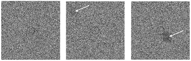
Figure 1. Detection task. Three examples of single trial presentations: Background raster only (left panel), a barely detectable foreground object indicated in the top-left field of the middle panel, and an obvious foreground object (right panel). A circle at the center of the image appeared in all trials of all sessions; the subjects were instructed to try to fixate on that circle at the beginning of each trial.

Stimulus Control and Estimation of Detection Probability

The experimental design was adopted from a recently introduced Response Clamp methodology for analysis of neural fluctuations (Wallach et al., 2011), with modifications that enabled its application to the present behavioral setting².

Response probability was estimated on-line as follows: Let s_n be an indicator function, so that s_n = 1 if the subject detected the n-th foreground stimulus and s_n = 0 otherwise. We define π(n) as the probability of the subject to detect a foreground stimulus at trial n. We can estimate this probability using all past responses by integrating them with an exponential kernel,

where τ is the kernel’s decay-constant. To compute this on-line, we used the recursive formula:

setting τ = 10 trials, and

A proportional–integral–derivative (PID) controller was realized in Wolfram’s Mathematica 7.0 environment. The input to the controller is the error signal,

where and are the desired and actual detection probabilities (calculated as explained below) at the n-th trial, respectively. The output of the controller is generally composed of three expressions,

where g_P, g_I, and g_D are the proportional, integral, and derivative gains, respectively; g_P was set to 1.0, g_I to 0.02, and g_D to either 0.02 or 0 (with no appreciable effect). Our experience has been that the integral component is essential: omitting that component results in stabilization around an arbitrary and time-variant value; for an extensive discussion on this issue see Figure 3D in Wallach et al. (2011), a methodology paper that introduces the concept of Response Clamp in the neural context.

Finally, the contrast C_n equals the controller’s output plus some baseline:

where

Fano-Factor Analysis

To quantify correlations in a given sequence of binary responses, the latter was divided to non-overlapping bins of size K. A count sequence Z_K was constructed by registering the number of positive responses (i.e., trials in which the visual object was detected) within each of the bins. This process was repeated for all bin sizes used. For each count sequence thus obtained, the Fano-factor (variance to mean ratio) is defined as F(K) = var(Z_K)/mean(Z_K) and plotted as a function of the bin size, K. As extensively established by Teich et al. (1997), this quantity provides a way to extract correlations in a sequence of binary events: An uncorrelated white process (e.g., Homogeneous Poisson Process) yields a constant F(K) for all bin sizes; regularity (e.g., low-jitter oscillation) would be reflected in a decreasing F(K) within the relevant range of bin sizes; and, finally, a complex temporal structure, exhibiting long-term correlations (e.g., fractal point process), would produce an ever increasing F(K), following a power-law relation to bin size.

Closed-Loop, Replay, and Fixed Contrast Modes

In the basic design, each subject was exposed to three experimental sessions denoted closed-loop, replay, and fixed. The first session was always a closed-loop session, whereas the second and third were replay and fixed sessions, introduced in an alternating order to different subjects. A 10-min break was given after the first and second sessions.

In the closed-loop session, the desired response probability () was kept constant ( unless indicated otherwise in the main text) and the control algorithm operated as explained above, updating the contrast (C_n) of the foreground object from one trial to the next based on the error signal (e_n). The series of 450 C_n values produced in this closed-loop session (500 trials minus the 50 sham trials), served for the generation of both dynamically and statistically identical foreground objects in the replay session. Thus, in the replay session the control algorithm was disconnected, yet we were able to record the responses of the subject to exactly the same series of contrasts presented in the closed-loop session, but now in an open-loop context, detached from the trial-by-trial coupled observer’s–observed dynamics. In the fixed session, the average contrast calculated from the series of above mentioned contrasts was used for all presentations, thus omitting stimulus variance altogether. This fixed session allowed us to estimate the impact of stimulus fluctuations on response dynamics.

Results

The nature of the detection task is demonstrated in Figure 1: The left panel shows a background raster only. The middle panel shows a barely detectable foreground object (indicated in the top-left field). The righthand panel demonstrates an obvious foreground object. The probability of false positive detection, calculated from responses of all subjects to the 50 sham trials was negligible (0.017, SD = 0.029, n = 8), indicating that the subjects did not tend to report detection when they did not really see something. The average response time was around 1 s per trial, slightly longer in the closed-loop session (1.03 s, SD = 1.3) compared to replay and fixed sessions (0.89 s, SD = 1.6 and 0.81 s, SD = 1.0, respectively). Response time distributions in all three sessions had a long right tail (coefficient of skewness: 11, 17, and 19, respectively).

The main observation is shown in Figure 2, where the responses of one subject (left column) and the group of eight subjects (right column) that were tested in closed-loop (dark blue, top row), replay (purple, middle row), and fixed (a kind of yellow, bottom row) sessions are plotted. Let us start with Figure 2A, describing the results obtained in the closed-loop session of one individual. The desired detection probability (see Materials and Methods) was set to 0.5, and the control algorithm updated the contrast C_n, trial-by-trial, as indicated by black dots (righthand y-axis of Figure 2A). The resulting estimated detection probability ( dark blue, lefthand y-axis) of that individual gradually approached the desired value, albeit fluctuating about it. Also note the expected anti-correlation of C_n and Figure 2B shows the average performance (and SD) of all eight subjects that participated in such a closed-loop session, showing that the controller converges within ca. 100 trials, and succeeds in “clamping” the detection probability at around 0.5, as preset.

FIGURE 2

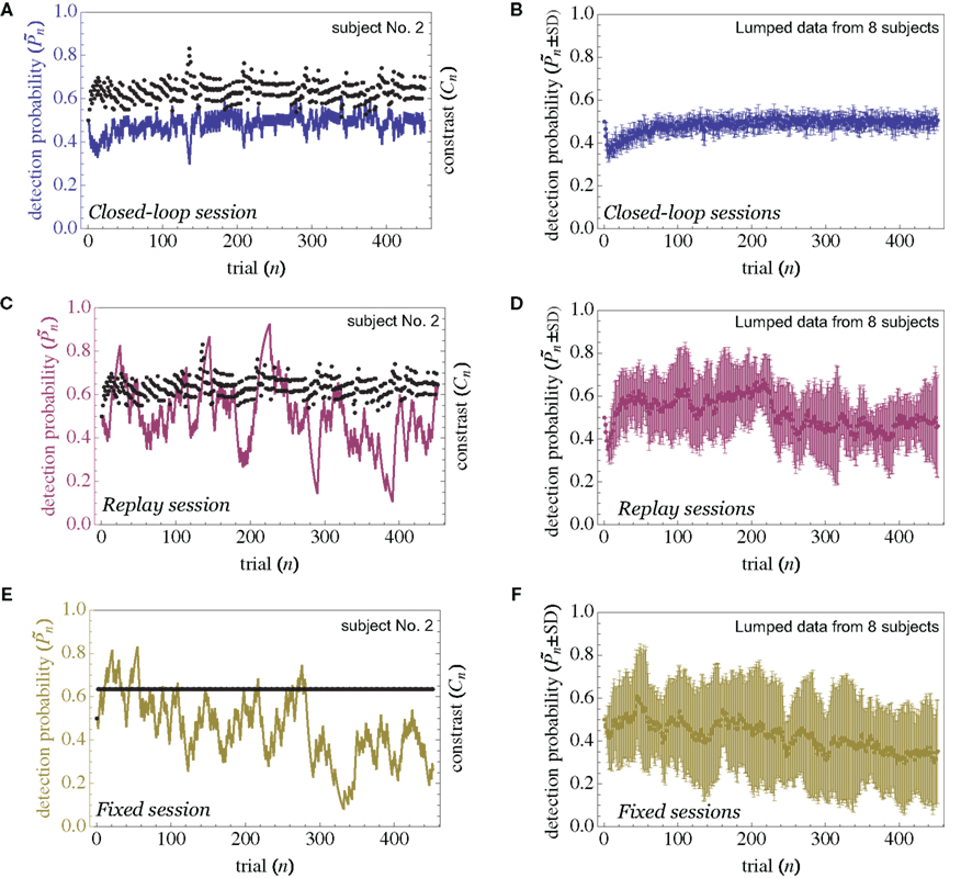
Figure 2. Detection probability in closed-loop, replay, and fixed sessions. Data obtained from an experiment on one individual (left column) and the summation of observations from the eight different subjects that were tested in this protocol (right column). In all cases, the fluctuations around mean detection probability are significantly smaller in the closed-loop session. The initial decline in detection probability, which is most apparent in the closed-loop and replay sessions, reflects the initial setting of both and C_n to 0.5. Error bars in the righthand column depict SD across all subjects.

Figure 2C shows the performance of the same individual whose data are shown in Figure 2A, but now in the replay session, where the C_n series obtained in the closed-loop session (black dots) is “replayed,” regardless of the subject’s responses. Under these conditions the control algorithm is shut down and stimulus contrast is completely decoupled from the subject’s behavior. Note the emergence of large slow fluctuations around the preset 0.5 detection probability; despite the fact that the stimulus series is practically identical to that shown in Figure 2A, the performance in Figure 2C is very different. Figure 2D shows the average performance (and SD) of all eight subjects that participated in the replay session.

And finally, as demonstrated in Figure 2E, when the average C_n of the subject – whose data is shown in Figures 2A,C – is used in the fixed session, where all 450 trials have identical contrast (black line of Figure 2E), large slow fluctuations and drift (which might reflect perceptual fatigue) are observed. Figure 2F shows the average performance (and SD) of all eight subjects that participated in these fixed session.

As mentioned in the introductory comments to this study, psychophysical data exhibits correlations over extended timescales in responses to near-threshold stimuli (Werthheimer, 1953; Gilden, 2001; Monto et al., 2008). Such long-term correlations are apparent in the open-loop data of Figures 2C,E. Figures 3A,B demonstrates one way to quantify the statistics of these correlations, using Fano-factor analyses (see Materials and Methods). It shows that both for the case of an individual subject (Figure 3A) as well as the lumped data of all subjects (Figure 3B), response fluctuations in the open-loop modes are indeed dominated by long-range correlations, whereas responses in the closed-loop (controlled) mode exhibit regularity, reflected as a decreasing Fano-factor within the observed bin sizes. Autocorrelation or, equivalently, power spectrum analyses also show substantial lessening of slow frequency components in the closed-loop mode (data not shown).

FIGURE 3

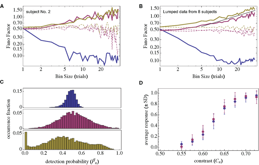
Figure 3. Temporal structure and psychometrics. (A,B) Fano-factor analysis (see Materials and Methods) for a single subject (A) and the average over eight subjects (B). Long-term correlations in the temporal fluctuations of responses in both the replay and fixed modes (solid lines, purple, and yellow, respectively) are revealed. A solid black line in (B) depicts power-law relations (exponent power of 0.4), for reference. Under the closed-loop conditions (solid dark blue line), the Fano-factor decreases as a function of bin size, indicative of a highly regular process. Random shuffling of the response sequences eliminates all temporal correlations, yielding (as expected) a constant Fano-factor (dashed lines). (C) Histograms of detection probability (), calculated from data of all subjects, in closed-loop (top), replay (middle), and fixed session. (D) Both threshold and sensitivity are practically identical in closed-loop (dark blue) and replay (purple) sessions. The curves were calculated by averaging the responses (1’s and 0’s), for each of the eight subjects, in different contrast (C_n) bins; bin size = 0.025. A minimum of five occurrences of a given contrast per bin was set as a requirement for inclusion in the calculation. The Average Response (y-axis) and its SD among subjects for each contrast bin are shown in the plot. Note that average response thus calculated is not the same quantity as detection probability (the latter takes into account the temporal order of responses).

The group statistics of Figures 2B,D,F are summarized in Figure 3C. Clearly, the best performance is obtained when relational dynamics are allowed between (the performance of the observer) and C_n (the contrast series). One possible explanation to this result is that under these different experimental conditions there is a change in the sensitivity of the subject to the stimulus. Figure 3D shows the psychometric functions for closed-loop and replay sessions, calculated by averaging the responses (1s and 0s), for each of the eight subjects, in different contrast (C_n) bins. (Note that average response thus calculated is not the same quantity as detection probability the latter takes into account the temporal order of responses.) Clearly, these psychometric functions show that both threshold and sensitivity extracted from the responses of all the subjects, are practically identical in closed-loop and replay. However, the richness of the dynamics and the marked differences between closed-loop and replay modes seen in Figures 2 and 3B, are practically averaged out when the data are collapsed to standard psychometric functions of the kind shown in Figure 3D.

The importance of instantaneous coupling between the observer’s behavior and the stimulus dynamics is demonstrated in Figure 4A, where a closed-loop mode is instantly switched to a fixed mode, by disconnecting the controller and using a constant contrast value (average of the C_n series over a time segment depicted by a black bar). Figure 4A shows data of a single subject, in three different preset values (0.25, 0.5, and 0.75). As soon as the coupling of observer’s–observed dynamics is disconnected, the variance of detection probability markedly increases and slow correlations seem to emerge, at all tested. As shown in the averaged histograms of Figure 4B, within the fixed phase of the experiment of Figure 4A the detection probabilities are skewed, exhibiting a “binary” preference toward 1 or 0 (for the cases of and respectively). This preference stands in contrast to the symmetric case of (e.g., Figure 3C).

FIGURE 4

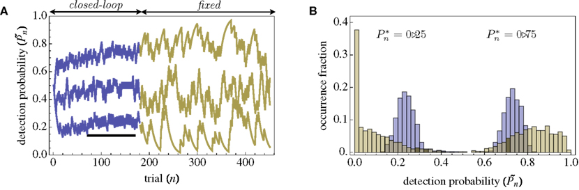
Figure 4. Responses of subjects to sudden transition from closed-loop to fixed modes. (A) A closed-loop mode is instantly switched to a fixed mode, by disconnecting the controller and using a constant contrast value (average of the C_n series over a time segment depicted by a black bar). Data obtained from a single subject in three different preset values (0.25, 0.5, and 0.75). (B) Average distributions of detection probability (n = 4 subjects) for and sessions as shown in (A); obtained separately from the closed-loop (blue) and fixed phases.

Conclusion

Two basic observations are presented here. The first is that trial-to-trial variability in sensory detection of a weak visual stimulus is dramatically diminished when rather than presenting a stimulus contrast that is independent of the subject’s ongoing actions, the fluctuations in stimulus contrast were matched to the fluctuations in a subject’s judgment. Clearly, this result reaffirms that trial-to-trial fluctuations are not “noise” in the strict sense of being independent of each other. Moreover, the significant difference, between features of fluctuations measured when dynamic observer–observed relations exist, and those measured in the absence of such coupled dynamics, calls for re-examination of the way psychophysical experiments are conducted. Indeed, measuring temporal fluctuations of a psychophysical function under open-loop conditions, where there is no relation between subject performances and sensory object contrast dynamics, is a most un-natural setting. Here we implemented an adaptive algorithm (PID) borrowed from control theory in order to couple the observer–observed dynamics. The PID control algorithm has theoretical advantages in the present context by being simple, and probably the most extensively used and theoretically studied in control engineering (Levine, 1996). Having said that, there exist many other adaptive psychophysical procedures (Treutwein, 1995) that are, actually, in use when experimentalists attempt to identify points of interest on psychometric functions. We propose to substantially extend their use in order to expose the dynamics of perception under more natural experimental conditions. The second basic observation is that the above diminishing of trial-to-trial fluctuations by coupling between observer–observed dynamics, is not accompanied by a change in sensory sensitivity to the input. Taken together, the two basic observations suggest that trial-to-trial variability in sensory detection of weak stimuli might reflect a high-level control process.

As pointed out by Werthheimer (1953), trial-to-trial variation at threshold was generally attributed, in the early days of psychophysics, to uncontrolled experimental conditions, with the assumption that the subject is stable. Response fluctuations, however, were soon shown to be non-independent (Verplanck et al., 1952); that is – successive responses to repeated presentations of the same threshold stimulus (in auditory, visual, and somatosensory modalities) are correlated over timescales ranging from seconds to days (Werthheimer, 1953). These long-range trial-to-trial response correlations were then interpreted as reflecting modulation of an a priori detection probability by recent subjective experience, a meta-cognitive guessing process that is active where there is no possibility for stimulus-determination; the assumption being that “guesses are more likely to be influenced by preceding responses (success and failures) than are sensory judgments” (Conklin and Sampson, 1956). Later years brought with them a more reductionistic focus on neural sources of “noise” and “short-term plasticity” that may account for observed trial-to-trial response variability (Faisal et al., 2008). Viewed from this historical angle, the results presented here pull the pendulum back to the meta-cognitive pole, offering an interpretation according to which – when facing a weak stimulus – subjects vary their response patterns, seeking to establish (predictive? see Rosen, 1985; Creutzig et al., 2009) relations between their actions and the dynamics of stimulus features. This interpretation, in its broader sense, goes far beyond psychophysics of weak stimulus detection; it touches upon what psychologists try to tell us over the past 50 years on the developing mind (e.g., Stern, 1985), when we care to listen.

Conflict of Interest Statement

The authors declare that the research was conducted in the absence of any commercial or financial relationships that could be construed as a potential conflict of interest.

Footnotes

1. ^Stimulus-determination is a term used by Conklin and Sampson (1956) as well as others to indicate the extent to which a subject’s response is determined by features of the stimulus itself, rather than stimulus-independent factors.
2. ^For an extensive discussion of parameter choices, the reader is encouraged to consult Wallach et al. (2011).

References

Conklin, J. E., and Sampson, R. (1956). Effect of stimulus-determination on response-independence at threshold. Am. J. Psychol. 69, 438–442.

Pubmed Abstract | Pubmed Full Text | CrossRef Full Text

Creutzig, F., Globerson, A., and Tishby, N. (2009). Past-future information bottleneck in dynamical systems. Phys. Rev. E Stat. Nonlin. Soft Matter Phys. 79(4 Pt 1), :041925.

Pubmed Abstract | Pubmed Full Text

Faisal, A. A., Selen, L. P. J., and Wolpert, D. M. (2008). Noise in the nervous system. Nat. Rev. Neurosci. 9, 292–303.

Pubmed Abstract | Pubmed Full Text

Gilden, D. L. (2001). Cognitive emissions of 1/f noise. Psychol. Rev. 108, 33–56.

Pubmed Abstract | Pubmed Full Text

Levine, W. (1996). The Control Handbook. Boca Raton, FL: CRC press.

Marom, S. (2010). Neural timescales or lack thereof. Prog. Neurobiol. 90, 16–28.

Pubmed Abstract | Pubmed Full Text

Monto, S., Palva, S., Voipio, J., and Palva, J. M. (2008). Very slow EEG fluctuations predict the dynamics of stimulus detection and oscillation amplitudes in humans. J. Neurosci. 28, 8268–8272.

Pubmed Abstract | Pubmed Full Text | CrossRef Full Text

Rosen, R. (1985). Anticipatory Systems: Philosophical, Mathematical, and Methodological Foundations. Oxford: Pergamon Press.

Stern, D. N. (1985). The Interpersonal World of the Infant: a View from Psychoanalysis and Developmental Psychology. New York: Basic Books.

Teich, M., Heneghan, C., Lowen, S., Ozaki, T., and Kaplan, E. (1997). Fractal character of the neural spike train in the visual system of the cat. J. Opt. Soc. Am. A Opt. Image Sci. Vis. 14, 529–546.

Pubmed Abstract | Pubmed Full Text

Treutwein, B. (1995). Adaptive psychophysical procedures. Vision Res. 35, 2503–2522.

Pubmed Abstract | Pubmed Full Text

Verplanck, W., Collier, G., and Cotton, J. (1952). Nonindependence of successive responses in measurements of the visual threshold. J. Exp. Psychol. 44, 273–282.

Pubmed Abstract | Pubmed Full Text

Wallach, A., Eytan, D., Gal, A., Zrenner, C., and Marom, S. (2011). Neuronal response clamp. Front. Neuroeng. 4:3. doi: 10.3389/fneng.2011.00003

CrossRef Full Text

Werthheimer, M. (1953). An investigation of the randomness of threshold measurements. J. Exp. Psychol. 45, 294–303.

Pubmed Abstract | Pubmed Full Text