A linear model of phase-dependent power correlations in neuronal oscillations

Introduction

Different situations may require different aspects of knowledge stored in the brain (Dayan et al., 2000). This adaptive knowledge selection can be achieved by enhancing the influence of a specific set of synapses. The selective use of certain synapses is a way to route information and to modulate communication between neurons. The communication through coherence (CTC) theory postulates that the communication between two neuronal populations is supported by the membrane potential phase difference between the oscillations in the two populations (Fries, 2005). This theory has been very influential because it confirms a role for oscillations in the neuronal code (Buschman and Miller, 2007; Knight, 2007; Saalmann et al., 2007; Womelsdorf and Fries, 2008; Fries, 2009; Tiesinga and Sejnowski, 2009; Hipp et al., 2011; Singer, 2011).

It has been tested experimentally by means of the phase difference between the multi-unit activity (MUA) from two recorded units, or between the MUA and the local field potential (LFP; Womelsdorf et al., 2007). To this end, for both recorded units, amplitude and phase of a given oscillation frequency were estimated on a trial by a trial basis. Interestingly, for those trials that had a phase difference similar to the mean phase difference (“good phase”) oscillation amplitudes were more strongly correlated than for those trials that had a phase difference not corresponding to the mean (“bad phase”).

In a recent paper (Buehlmann and Deco, 2010), a biophysically plausible semi-large-scale model was built on the results of Womelsdorf et al. (2007). In the present work, we have developed a simpler linear model in order to try to understand what the main principles defining the relationship between oscillation amplitude correlations and phase differences are. We found that a linear interaction between oscillators can qualitatively fit the experimental results, which allowed us to extract several analytical predictions. These basic principles could then be applied to understand phase-dependent amplitude statistics in spiking activity and in LFP, EEG, and MEG (Wendling et al., 2009).

Materials and Methods

Model

The model consists of two interacting units represented by variables, O_a and O_b, each of which correspond to a narrow-band filtered LFP or MUA around a given frequency. We assume that the interaction is linear, and in general, described by the sum of a remote and a local oscillatory component. The governing equations are written as

A^k(t) and B^k(t) denote the amplitude of unit A and B before any coupling occurs at the k-th trial. O_a(t) and O_b(t) without the trial superscript k will be used to denote the output in general. f_a and f_b denote the frequencies of interest in unit A and B. τ is the conduction delay between unit A and B. Notice that conduction delays of cortico-cortical long-range connections have been measured to amount up to several tens of milliseconds (Swadlow and Waxman, 1975; Swadlow, 1985; Nadasdy, 2009). Therefore, it may be important to take the conduction delay into account in order to define the good phase (for a definition of the good phase see Power and Phase Estimation in the Analysis part in the Materials and Methods). w_{I → J} is the connection strength from unit I to unit J. Δφ denotes the phase difference between O_a(t) and O_b(t) when the connection strengths are zero, we name this phase difference the uncoupled phase difference.

We would like to stress that the model described by Eqs 1 and 2 together with its parameter settings is not intended to represent the actual interference of the electric fields generated at two different brain areas. Rather it should be viewed as an abstraction of a linear and phase-dependent coupling of two oscillatory processes.

Settings for the Simulations

Simulations with stationary parameters

Two different cases of stationary parameters were simulated according to the distribution of the amplitudes over trials:

(i) All the variables of the model, A(t), B(t), and Δφ(t), were constant in time during one trial and could be described by A, B, and Δφ. w_{b → a}was set to 0 and w_{a → b} was referred to as w. Only one period was simulated with 100 time points. For the realizations over trials A and B were drawn from a uniform distribution from 0 to 1. The phase difference, Δφ, was drawn from a −π to π uniform distribution. For simplicity τ was set to 0 and w(f) was set to 1. These settings were also used in the section of analytical predictions.

(ii) For the variables, A(t), B(t), and Δφ(t), w_{b → a}, w_{a → b} see (i). The realizations A and B were drawn from a Gaussian distribution with a SD one and mean zero. The values for the variables in Eq. 2 were set to the following. We randomized 50,000 amplitude pairs A^(k) and B^(k), and 50,000 Δφ^(k), i.e., k = 1.50000. The time t was run from 0 to 2π in steps of 0.1, i.e., the simulation was run for one period. For simplicity τ was set to 0.

Simulations with Non-Stationary Parameters

This changing parameter-set was chosen to test the timing of the establishment of a “good” phase relationship relative to the increase in power correlation. A trial of 120 time points was defined with 1 ms resolution per time point. The period of oscillations was set to 20 ms. The time resolved phase relation was calculated as cos(Δ − δ), where δ is the phase accumulated due to the conduction delay, and Δ is the phase difference between the coupled model variables O_a(t) and O_b(t) at time t (cos(Δ − δ) = 1 or −1 for the “good” or “bad” phase, respectively). The amplitudes for both recorded units were always kept constant during this time period, but were drawn from a Gaussian distribution for different repetitions, independently for the two units. Repeated simulations with different amplitudes were necessary in order to estimate the power correlation for every time point. The power correlation at each time point was estimated across 200 repetitions. The phase relation was always the same across repetitions.

Analysis

Power and phase estimation

In simulations, the phase and amplitude were calculated using a windowed fast Fourier transform. The window was rectangular and had a duration corresponding to one period. The amplitude and phase of the signal, y, at time t will be referred to as |fft(y,t)| and φ(fft(y, t)), respectively, where |x| = |a + ib| = √(a² + b²) and φ(x) = arg(a + ib). The good phase was defined as the mean phase, i.e., φ(), where N denoted the number of trials. The power was calculated as |a + ib|².

Estimation of power correlation, mutual information, and modulation depth

To estimate the phase-dependent power correlation (PDPC), amplitude, and phase for O_a(t) and O_b(t) were estimated in a 2π− wide window centered around π, i.e., from 0 to 2π. According to Womelsdorf et al. (2007), the phase difference was divided into six equally sized bins. The power correlation was then calculated as the Pearson coefficient for the powers of those trials that had phase differences belonging to the same bin.

Mutual information between the amplitudes of O_a(t) and O_b(t) was calculated using a bias-corrected “naive histogram” estimate (computed via the Matlab function “information.m,” available from http://www.cs.rug.nl/∼rudy/matlab/doc/information.html). For each bin of the phase difference the mutual information was calculated on 3000 pairs (in the bad/good phase bin there were around 5000/16000 pairs) that were drawn with replacement. The mean of the information in each bin was calculated on 1000 repetitions.

The modulation depth is the peak-trough distance, where peak corresponds to the maximal power correlation and trough corresponds to the minimal power correlation.

Results

First, using analytical derivations, we will examine the characteristics of the PDPC for oscillators interacting with uni-directional, bidirectional, and common drive connectivity. Using results from the analytical study, we predict that the width of the phase dependency will be different for the uncoupled and the coupled phase difference. This is tested with numerical simulations. Using numerical simulations we also examine if the power correlation lags the phase difference, i.e., if the phase difference plays a causal role in determining the power correlation. Finally, we summarize the results using a non-linear correlation index such as mutual information.

Analytical Derivations and Predictions

In this section, we compute how power correlations between two linearly coupled oscillatory processes depend on their phase difference and coupling strength. We start by considering the case of uni-directionally coupled oscillators by setting w_{b → a} = 0 (see Eqs 1 and 2) and denoting w_{a → b} with w. We set the amplitudes A and B fixed in time and only depending on the trial realization.

We first proceed by relating the amplitude of process O_b(t) (the receiver) to that of process O_a(t) (the emitter) and the coupling coefficient, w. Once such a relation is established we can compute the Pearson correlation coefficient between the powers of the two processes. This holds, regardless of the particular distribution from which the amplitudes over trials are drawn. For simplicity, we will illustrate here the case where the amplitudes are sampled from a uniform distribution covering from 0 to 1.

We proceed by computing the amplitude of process O_b(t). We use the fact that process O_b(t) is the sum of two harmonic processes, and therefore, it is itself a harmonic process. Thus, the modified (after being coupled) amplitude D and phase θ of process B can be obtained by solving the equation

For each trial, this leads to a new amplitude D and phase difference θ that read

and

Eq. 7 demonstrates how the amplitude difference (wA/B) can modulate the phase difference (see Figure A1 in Appendix). Since we are interested in the power correlation between the two processes we are left to compute the Pearson coefficient between D² and A²

where E[] denotes the expected value operator

and p(X) is the probability density function of a real random variable X.

In this simplified model we assume that from trial to trial the amplitudes A and B are drawn from a uniform distribution. Since A² and D² are functions of A and B, it is possible, in principle, to compute the probability density functions that A and B induce on each of the powers and later compute the integrals appearing in Eq. 8. However, since we are only interested in the expected values a much more practical approach is to use the fact that

and its analog version for functions of multiple random variables. After computing the integrals appearing in Eq. 8 the Pearson correlation coefficient between the powers A² and D² as a function of the coupling strength and phase difference can be obtained as

Now, it is possible to study with more detail how power correlations are due to different coupling characteristics. For example, from the formula above it can be deduced that the maximum of the power correlation grows with the coupling strength monotonically. However, the phase difference for which this maximum arises presents a switching point for a coupling strength w ≈ 0.95 (Figure 1A). Below that critical coupling strength, the maximum of the power correlation is achieved at a zero phase difference (Δφ = 0). When the coupling strength is larger than ∼0.95, there is a double maximum which in the case of large coupling strength limit occurs for phase differences of Δφ = ± π. Additionally, one can observe that negative power correlations can arise for certain phase differences only if the coupling is below the critical strength. (Note, however, that a Gaussian amplitude statistics, in contrast to a uniform amplitude statistics, in general generates a more positive correlation for the bad phase, see Figure A2 in Appendix). Beyond that limit only positive correlations arise, no matter the phase difference.

FIGURE 1

Figure 1. Analytical results. (A) Power correlation as a function of the uncoupled phase differences for a range of connection strengths (color coded). For comparison with the experimental results of Womelsdorf et al., 2007, we have plotted a cosinus function that is vertically translated to not interfere with the PDPC curves. (B) Bidirectional coupling for five different delays (color coded). Coupling strength w = 0.3. Uniform distribution of uncoupled amplitudes over trials. Note that the lowest correlation (bad phase) can be around 90° for some delays.

The former analysis considered a uni-directional type of interaction between units. Cortical connectivity is, however, much more often bridging areas in a bidirectional or reciprocal manner. Next, we explore therefore how power correlations arise in a bidirectional scheme of coupled oscillations. For the bidirectional case, w_{b → a} > 0 see Eqs 1 and 2), the analysis proceeds as described for the uni-directional one, except for one distinction, namely, that the phase difference between the oscillators is composed by an initial phase difference and a propagation phase due to a delay in the interaction. In the uni-directional case, these two contributions could be simply added into a single term rendering the individual contribution of each indistinguishable. In the reciprocal case, axonal delays add a factor that strongly modifies the shape of the power correlation curve. The interacting oscillators are now described by

whereby both powers depend explicitly on the phase propagation accumulated due to axonal delay in addition to the initial phase difference. They read as

The power correlation can now be computed as a function of different variables from the expected values appearing in Eq. 8 once A is replaced by the expression of the new power C. The analytical expression for the power correlation curve can be obtained even for asymmetric values of the coupling strengths w_{b → a} ≠ w_{a → b} and reads

Figure 1B displays the analytical results for the power correlation versus the uncoupled phase difference in a bidirectional interaction of oscillations. The Figure illustrates the symmetric and moderate coupling case for which we have considered different axonal delays. Clearly, the delay does not simply shift the curve but modifies its shape indicating that axonal conduction delays have to be taken into account when interpreting power correlation curves from experimental data.

Distinct neuronal units can also share power correlations without directly interacting. Common drive from a third source can create PDPCs between the driven units as it occurs described for uni-directional and bidirectional interactions. A distinction of the two scenarios is relevant to assess the origin of the phase-dependent correlations in neurophysiological recordings. In general, we observe that correlations generated by the three topologies qualitatively differ in terms of their dependency of the connection strength (see Appendix and Figure A3).

Power Correlation as a Function of the Coupled Phase Difference

Overall, the phase dependency in Figure 1A is broader compared with the one for the experimental data. This could be because the experimental data exhibit a coupled phase difference (θ) rather than an uncoupled one (Δφ). In principle, Eq. 7 relates the coupled phase difference to the uncoupled one but lamentably such dependency is not one-to-one since A and B are not fixed from trial to trial. Therefore, one cannot translate directly from the uncoupled to the coupled phase difference. It is possible, however, to relate them in a statistical sense. To that end, we integrate θ over the random distributions of A and B to obtain an average coupled phase difference as a function of the uncoupled one,

The numerical estimation of such integral shows that for a moderate coupling strength the average phase difference depends almost linearly on the uncoupled one (Figure 2A). Therefore, it is expected that power correlations as a function of the coupled phase look similar to Figure 1A but with the phase difference axis scaled by a numerical factor. Indeed, the power correlation curve becomes narrower when the power correlation is calculated as a function of the coupled phase difference instead of the uncoupled phase difference (Figure 2B and see Figure A4 in Appendix). A similar result is obtained when power is estimated instead of amplitude and when Spearman rank correlation is used instead of Pearson correlation (data not shown).

FIGURE 2

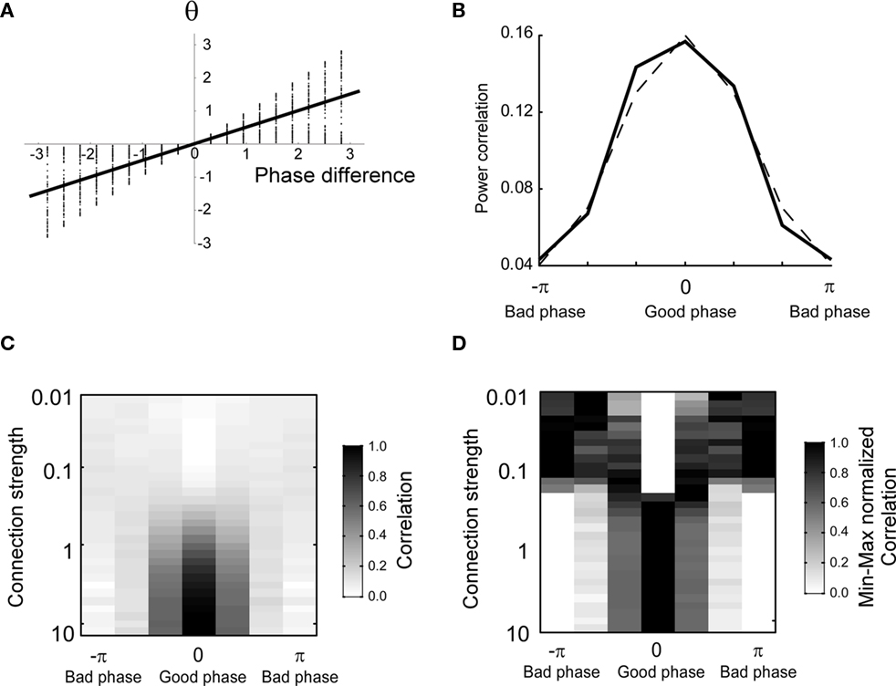
Figure 2. The shape of the phase-dependent power correlation is changed when the coupled phase is regarded rather than the uncoupled phase. The amplitude distribution is Gaussian. (A) Relation between the averaged coupled and the uncoupled phase difference. Note that the slope of the regression line is 0.5. Thereby, the uncoupled phase difference is compressed as it is transformed into the coupled phase difference. (B) Comparison between the phase-dependent power correlation for connection strength of 0.3 and a cosine. (C) Correlation as a function of phase and connection strength. (D) Maximum normalized correlation as a function of phase and connection strength.

The shape of the PDPC was also found to be dependent on the connection strength (Figure 2C). The shape of the PDPC can be better visually inspected after dividing the PDPC by its maximal value. For large connection strengths we observe that the normalized shape stabilized (Figure 2D).

Next, we examined how the modulation depth (see Analysis subsection in the Materials and Methods) of the PDPC and the strength of the phase coherence scale with different connection strengths (Figure 3). This is of particular interest because according to Womelsdorf et al. (2007, their Figures 1 and 2), there exist cases in which the two can dissociate; a relatively high phase coherence not always predicts a PDPC. Indeed, one can observe how for low coupling strengths (∼0.2) there is a regime where phase coherence can coexist with an almost flat or slightly negative peaked PDPC curve (Figure 3). However, at higher connection strengths an overall positive correlation between phase coherence and modulation depth is found.

FIGURE 3

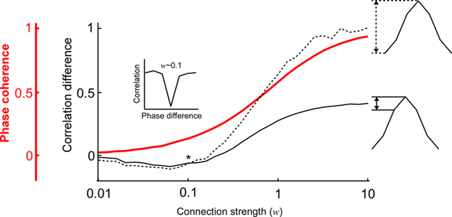
Figure 3. The relation between the phase coherence and the shape of the coupled phase-dependent power correlation depends on the connection strength. The shape of the coupled phase-dependent power correlation was quantified either using the correlation difference between the 0 and π phase difference (dashed black line) or the correlation difference between the 0 and π/3 phase difference (solid black line). The two correlation difference curves intersect when the connection strength is approximately 0.1 (indicated by an asterix *). Therefore, correlations for π and π/3 are approximately identical (see inset). Note that the good phase has lower correlations than the bad phase despite the phase coherency is larger than 0.1 (red line).

The Timing of Phase Relations and Power Correlations

The experimental results have shown that a good phase relationship precedes a strong power correlation as shown in Figure 3 of Womelsdorf et al. (2007). Such a lag could indicate a causal role for the phase relation in modulating the efficacy of the interaction as measured by power correlations. In order to examine this question we have introduced a sudden change in the phase relation (perturbing the phase in unit A) from a bad phase to a good phase at 60 ms, and back to a bad phase at 80 ms (Figure 4A). For a connection delay of 4 ms, the peak of the power correlation is delayed by approximately 4 ms relative to the maximum of the phase relation. The connection delay is correlated with the power correlation lag (Figure 4B). Since the power correlation lag is around 5 ms in the experimental data, this suggests that the average connection delay for the connection studied is in the range of 5 ms.

FIGURE 4

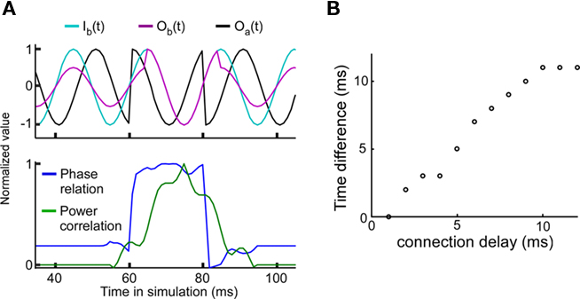
Figure 4. Good phase is followed by high power correlation. The connection strength is equal to 0.3. (A) A strong power correlation is preceded by a high coupled phase relation. Connection delay is 4 ms. Top panel: Background signal in unit A, I_a(t) = O_a(t) (black), background signal in unit B, I_b(t) (light blue), and “measured” signal in unit B with O_b(t) = w(f)O_a(t-T/2πf) + I_b(t) (cerise). Note that the amplitude of O_b(t) is larger during the good phase between 60 and 80 ms. Bottom panel: Normalized phase relation (blue) and normalized power correlation (green) for the same parameters. For the normalized phase relation values one corresponds to a good phase relation and zero corresponds to a bad phase relation. (B) The temporal lag of the power correlation relative to the phase relation is correlated with the connection delay.

Extending the Linear Correlation Analysis to a Non-Linear Information Index

The Pearson correlation measures the degree of linearity and the Spearman rank correlation the monotonicity between two variables. However, two variables can share information by being related in a more complex manner. Mutual information will now be used to characterize the relationship between oscillatory variables since it is essentially free from any assumptions required for the above mentioned correlation measures. In Figure 5A, we have plotted the mutual information for three different cases as a function of the uncoupled phase difference. When mutual information is calculated between O_b(π/(4f)) and O_a(π/(4f)), i.e., at a fixed point in time, and therefore without the non-linear amplitude extraction, the information for the bad phase is equal to that for the good phase condition. In contrast, when the amplitude is extracted, most information for both uniform and Gaussian amplitude distributions is retrieved specifically at the good phase. This is explained by the fact that amplitude (power) extraction is a non-linear operation that averages out correlations occurring between the instantaneous outputs at a given point in time. Moreover, the Gaussian distribution gives rise to a larger relative difference between bad and good phase than the uniform distribution.

FIGURE 5

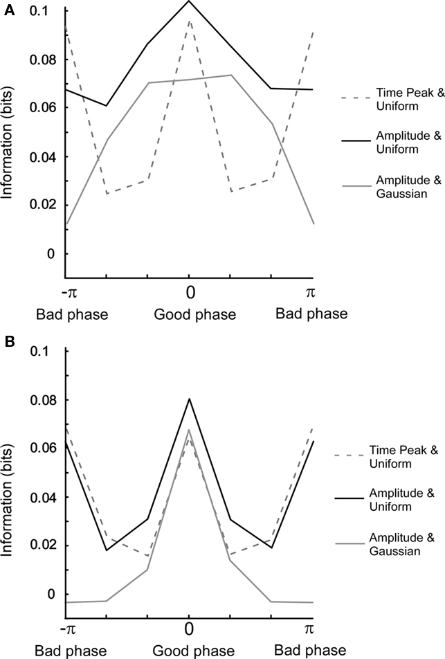
Figure 5. Mutual information for different settings of the model. (A) Uncoupled phase. The connection strength is 0.3. The x-axis (columns) denotes a phase difference in six bins. For a uniform amplitude distribution, correlations were calculated for both one time point amplitude (t = π/(4f)) and full period amplitude. For Gaussian amplitude distribution, correlations were calculated for full period amplitude. Note that the mutual information for the good phase is equal to that of the bad phase. (B) Same as in (A) but with coupled phase. Note that the full width half maximum is narrower in (B) than in (A).

When comparing model results for the coupled phase, the most prominent change is that the phase dependency becomes bi-modal for amplitude extraction and a uniform amplitude distribution (see Figure 5B). This is related to the fact that the tails of the power correlation curve as a function of the coupled phase difference take negative values (Figure A4B in Appendix). Since positive and negative correlations contribute equally to mutual information, a double peak is present when measuring mutual information versus the coupled phase difference.

Overall, the width of the mutual information based phase dependency is narrower than that of the correlation based. Furthermore, we have seen that the width is different between uncoupled and coupled phase differences. In Figure A5 in Appendix, we present a model that illustrates that the width can be of importance in particular for contrast dependent modulation of long-range lateral connections.

Discussion

We apply a model using a linear, albeit conduction delay dependent, neuronal interaction to examine how power correlations depend on phase differences and other parameters of oscillatory activity. Because of the simplicity of the model, the presented results are predicted to apply to generic interactions between oscillatory populations. Interestingly, the linear model leads to similar results as recently published experimental data. According to the model the influence of the connection makes one particular phase difference more frequent than other phase differences. This phase difference corresponds to the mean phase and it is referred to as the “good” phase. Since the mean phase emerges from the connection it is also a marker of the effective connectivity. Thus, it is argued that such phase might be responsible of generating the largest power correlations. In addition to explaining the experimental results the main contribution of the model has been the examination of how different parameters are influencing the shape of the phase dependency. The characteristics of the phase dependency have been investigated as a function of the correlation measure (non-linear versus linear), amplitude distribution, directionality, and of the nature of the phase difference (uncoupled or coupled).

Assumptions of the Linear Model

Our model is approximate and makes three main assumptions, i.e., the interaction is linear, and the input is sinusoidal and spatially uncorrelated. Here, we discuss those three assumptions. First, even though a linear model might not be biophysically plausible, linearity might be included as a main component of the interaction between postsynaptic potential and membrane potential. The relative contribution of that linear component decreases, however, when neighboring synapses are activated (Polsky et al., 2004), and certain types of theoretical models do not even consider a linear component (Rabinovich et al., 2008). Thus, a future approach extending our model should demonstrate how the phase dependency changes when different types of biophysical non-linearities are taken into consideration.

Second, we used a sinusoid as the oscillatory carrier to simulate the input since the sinusoid is the eigenfunction of the Fourier transform which was used to estimate the power. Power and phase of recorded signals are typically estimated around a particular frequency by using a narrow-band-pass filter. Therefore, the processed oscillatory activity is almost sinusoidal. The exact type of oscillator, however, does not matter since the results presented here hold for any periodic random function (data not shown).

Finally, we assume that the uncoupled activities of the units are independent. Such an assumption can be expected to hold for spatially distant neuronal populations (Smith and Kohn, 2008; Ecker et al., 2010). In reality, the spatial correlation length is probably limited to the minimal distance between two phase-independent oscillators. The upper limit of this distance has been estimated around 0.65 mm (Womelsdorf et al., 2007, their Figure 4).

Implications for the Investigation of Non-Linearities

Here, we have shown that a linear model can fit some recent experimental results concerning power correlation dependencies. Within a linear model information transmission can be reliably controlled if the noise amplitude is proportional to the signal, i.e., multiplicative noise. For example, if the DC level of the signal is decreased the noise would decrease too. If, on the other hand, the noise source is additive the signal would have to be amplified in order for the signal to noise ratio to increase, i.e., gain control (Haider and McCormick, 2009). Amplification, however, is a non-linear mechanism. If phase modulation is therefore proposed as a gain control mechanism it must operate in a regime that deviates from linearity. Here, we present the linear reference for such a comparison. The experimentally retrieved PDPC can be compared to a predicted PDPC. The only variable that is needed for that prediction is the connection strength, which in a strict sense can be estimated from the experimentally measured phase coherence.

A direct test for a non-linear relationship between phase and input has been done by TMS stimulation in the motor cortex while measuring the spinal input: “This enabled us to test whether the phase of the spinal beta rhythm at which the input arrived modulated the gain of this input” (van Elswijk et al., 2010). The authors describe that a naturally occurring beta rhythm is strong enough to change the gain of the spinal input. Oscillations slower than beta frequency have also been shown to modulate the cortical gain of sensory input (Lakatos et al., 2005; Lakatos et al., 2007; Rajkai et al., 2008). These studies point out the existence of some non-linear interactions at low frequencies between peripheral nerve systems and either sensory or motor cortex. However, the effect of such non-linearities on gamma power correlation statistics across cortical areas has still to be measured under physiological conditions.

Is a High Power Correlation Indicative of Causality?

Although, we have simulated here a case where – by construction – the phase has a causal role in power correlations, we would like to mention that in other scenarios, especially in more realistic setups, different interpretations of their lag are possible. First, the phase and amplitude of many oscillatory processes are intimately and mutually linked, and it is therefore not easy to assign a causal role to only one of the two variables. For instance, a perturbation in the phase of an oscillator can modify its amplitude, and vice versa. Further, the two variables can have a different inertia to perturbations, and therefore, temporal lags cannot be univocally interpreted as a sign of causality. Second, different measuring indices (e.g., phase differences and power correlations) can have different bias to detect the timing of perturbations. For example, in the presence of conduction delay T, it will take T ms until the effect of a sudden perturbation in A can reach unit B. If both phase and amplitude have been perturbed in A, the instantaneous phase difference will pick up such a change immediately. However, it might take some time around T for the variables at B to follow the change in A and build up some significant correlation with those at A. Thus, phase differences can precede power correlations even if the amplitude variable can have a causal role.

Related to the causality question is the fact that both common drive and direct interactions provide phase-dependent correlation curves. However, as we have seen there are qualitative differences between the PDPC for different topologies (Figure A3 in Appendix). For uni-directional topology and low connection strength, the correlation at zero phase difference is lower than that of the π phase difference (Figure A3B in Appendix). In contrast, for high connection strength, the correlation at π phase difference is lower than that of the zero phase difference. For the common drive topology, the correlation at π phase difference is lower than that of the zero phase difference, irrespective of connection strength (Figure A3D in Appendix). Therefore, the two topologies show differences in terms of the effect of the connection strength. In an experimental condition, however, we do not know the “connection strength” between two recording points. Instead, to disambiguate between the two topologies, we can use the experimentally measurable phase coherence as a correlate of the connection strength since we show that the two are monotonically related.

How a Connection Delay could Modulate the Proportion between Feed-Forward and Lateral Connections

For firing rates, it has been observed that the influential radius of lateral connections decreases when the contrast increases (Sceniak et al., 1999; Nauhaus et al., 2009). One could argue that if the stimulus has a high-contrast it needs little interpretation and therefore only weak lateral interactions, i.e., the feed-forward pathway is sufficient. However, if the stimulus were less salient, lateral connections would be required to obtain a meaningful interpretation of the stimulus.

Could this feed-forward–lateral modulation be transmitted by neuronal oscillations?

The feed-forward pathway has, according to modeling studies, been shown to benefit from strong gamma coherence and synchrony (Tiesinga et al., 2004; Buehlmann and Deco, 2010). Long-range lateral connections could be rendered ineffective if their delay generates a bad phase relative to a globally synchronized oscillation. Experimental evidence for such a delay-mediated and possibly contrast-controlled modulation of lateral connections can be drawn from several studies that show the presence of oscillations for high-contrast stimulation together with global synchrony and suitable delayed interactions. First, stimulus-contrast has been associated with gamma oscillations because increasing the contrast, or the mere introduction of a stimulus, enhances the amplitude of gamma oscillations (Fries et al., 2001; Henrie and Shapley, 2005; Lima et al., 2010; Yu and Ferster, 2010). Second, it has been shown that distant neurons can be globally synchronized for a high-contrast stimulus (Konig et al., 1995). Finally, as the largest distance between two laterally connected neurons within one cortical area is roughly 3 mm (Fisken et al., 1975; Gilbert and Wiesel, 1979; Rockland and Lund, 1982; Luhmann et al., 1990b), and the typical conduction velocity is around 0.3 mm/ms (Luhmann et al., 1990a; Hirsch and Gilbert, 1991; Murakoshi et al., 1993; Bringuier et al., 1999; Nauhaus et al., 2009), the largest connection delay is around 10 ms. Interestingly, this delay is relatively close to half the period of a 60-Hz gamma cycle (Fries et al., 2001; Womelsdorf et al., 2007). Therefore, globally synchronized distant (2–3 mm) neurons will accumulate a propagation phase close to the bad phase.

Essential for such a mechanism would be, however, the shape of the phase difference dependency. Assuming a constant conduction velocity this shape can be directly superimposed onto the cortical surface to delineate the functional extent of horizontal connections. Therefore, a crucial parameter returned by our model is the tuning width of the phase dependency (see Figure A5 in Appendix). Preferentially, the tuning width should be such that it maximizes the dynamic range of the horizontal connections.

Author Contribution

The study was conceived by David Eriksson. The numerical simulations were made by David Eriksson. The paper was written by David Eriksson, Raul Vicente and Kerstin Schmidt. The analytical solutions and predictions were derived by Raul Vicente.

Conflict of Interest Statement

The authors declare that the research was conducted in the absence of any commercial or financial relationships that could be construed as a potential conflict of interest.

Acknowledgments

We thank the reviewers for their valuable comments and suggestions to improve the paper. We thank Pascal Fries and Gilad Silberberg for comments on the early versions of the model, Wei Wu, Katharina Schmitz, Thomas Wunderle, and Peter Latham for comments on the manuscript.

References

Bringuier, V., Chavane, F., Glaeser, L., and Frégnac, Y. (1999). Horizontal propagation of visual activity in the synaptic integration field of area 17 neurons. Science 283, 695–699.

Pubmed Abstract | Pubmed Full Text | CrossRef Full Text

Buehlmann, A., and Deco, G. (2010). Optimal information transfer in the cortex through synchronization. PLoS Comput. Biol. 6, e1000934. doi: 10.1371/journal.pcbi.1000934

Pubmed Abstract | Pubmed Full Text | CrossRef Full Text

Buschman, T. J., and Miller, E. K. (2007). Top-down versus bottom-up control of attention in the prefrontal and posterior parietal cortices. Science 315, 1860–1862.

Pubmed Abstract | Pubmed Full Text | CrossRef Full Text

Dayan, P., Kakade, S., and Montague, P. R. (2000). Learning and selective attention. Nat. Neurosci. 3(Suppl.), 1218–1223.

Pubmed Abstract | Pubmed Full Text | CrossRef Full Text

Ecker, A. S., Berens, P., Keliris, G. A., Bethge, M., Logothetis, N. K., and Tolias, A. S. (2010). Decorrelated neuronal firing in cortical microcircuits. Science 327, 584–587.

Pubmed Abstract | Pubmed Full Text | CrossRef Full Text

Fisken, R. A., Garey, L. J., and Powell, T. P. (1975). The intrinsic, association and commissural connections of area 17 on the visual cortex. Philos. Trans. R. Soc. Lond. B Biol. Sci. 272, 487–536.

Pubmed Abstract | Pubmed Full Text | CrossRef Full Text

Fries, P. (2005). A mechanism for cognitive dynamics: neuronal communication through neuronal coherence. Trends Cogn. Sci. (Regul. Ed.) 9, 474–480.

Pubmed Abstract | Pubmed Full Text | CrossRef Full Text

Fries, P. (2009). Neuronal gamma-band synchronization as a fundamental process in cortical computation. Annu. Rev. Neurosci. 32, 209–224.

Pubmed Abstract | Pubmed Full Text | CrossRef Full Text

Fries, P., Reynolds, J. H., Rorie, A. E., and Desimone, R. (2001). Modulation of oscillatory neuronal synchronization by selective visual attention. Science 291, 1560–1563.

Pubmed Abstract | Pubmed Full Text | CrossRef Full Text

Gilbert, C. D., and Wiesel, T. N. (1979). Morphology and intracortical projections of functionally characterised neurones in the cat visual cortex. Nature 280, 120–125.

Pubmed Abstract | Pubmed Full Text | CrossRef Full Text

Haider, B., and McCormick, D. A. (2009). Rapid neocortical dynamics: cellular and network mechanisms. Neuron 62, 171–189.

Pubmed Abstract | Pubmed Full Text | CrossRef Full Text

Henrie, J. A., and Shapley, R. (2005). LFP power spectra in V1 cortex: the graded effect of stimulus contrast. J. Neurophysiol. 94, 479–490.

Pubmed Abstract | Pubmed Full Text | CrossRef Full Text

Hipp, J. F., Engel, A. K., and Siegel, M. (2011). Oscillatory synchronization in large-scale cortical networks predicts perception. Neuron 69, 387–396.

Pubmed Abstract | Pubmed Full Text | CrossRef Full Text

Hirsch, J. A., and Gilbert, C. D. (1991). Synaptic physiology of horizontal connections in the cat’s visual cortex. J. Neurosci. 11, 1800–1809.

Pubmed Abstract | Pubmed Full Text

Knight, R. T. (2007). Neuroscience. Neural networks debunk phrenology. Science 316, 1578–1579.

Pubmed Abstract | Pubmed Full Text | CrossRef Full Text

Konig, P., Engel, A. K., Roelfsema, P. R., and Singer, W. (1995). How precise is neuronal synchronization? Neural Comput. 7, 469–485.

Pubmed Abstract | Pubmed Full Text | CrossRef Full Text

Lakatos, P., Chen, C. M., O’Connell, M. N., Mills, A., and Schroeder, C. E. (2007). Neuronal oscillations and multisensory interaction in primary auditory cortex. Neuron 53, 279–292.

Pubmed Abstract | Pubmed Full Text | CrossRef Full Text

Lakatos, P., Shah, A. S., Knuth, K. H., Ulbert, I., Karmos, G., and Schroeder, C. E. (2005). An oscillatory hierarchy controlling neuronal excitability and stimulus processing in the auditory cortex. J. Neurophysiol. 94, 1904–1911.

Pubmed Abstract | Pubmed Full Text | CrossRef Full Text

Lima, B., Singer, W., Chen, N. H., and Neuenschwander, S. (2010). Synchronization dynamics in response to plaid stimuli in monkey V1. Cereb. Cortex 7, 1556–1573.

CrossRef Full Text

Luhmann, H. J., Greuel, J. M., and Singer, W. (1990a). Horizontal interactions in cat striate cortex: II. A current source-density analysis. Eur. J. Neurosci. 2, 358–368.

CrossRef Full Text

Luhmann, H. J., Singer, W., and Martínez-Millán, L. (1990b). Horizontal interactions in cat striate cortex: I. Anatomical substrate and postnatal development. Eur. J. Neurosci. 2, 344–357.

CrossRef Full Text

Murakoshi, T., Guo, J. Z., and Ichinose, T. (1993). Electrophysiological identification of horizontal synaptic connections in rat visual cortex in vitro. Neurosci. Lett. 163, 211–214.

Pubmed Abstract | Pubmed Full Text | CrossRef Full Text

Nadasdy, Z. (2009). Information encoding and reconstruction from the phase of action potentials. Front. Syst. Neurosci. 3:6. doi: 10.3389/neuro.06.006.2009

Pubmed Abstract | Pubmed Full Text | CrossRef Full Text

Nauhaus, I., Busse, L., Carandini, M., and Ringach, D. L. (2009). Stimulus contrast modulates functional connectivity in visual cortex. Nat. Neurosci. 12, 70–76.

Pubmed Abstract | Pubmed Full Text | CrossRef Full Text

Polsky, A., Mel, B. W., and Schiller, J. (2004). Computational subunits in thin dendrites of pyramidal cells. Nat. Neurosci. 7, 621–627.

Pubmed Abstract | Pubmed Full Text | CrossRef Full Text

Rabinovich, M., Huerta, R., and Laurent, G. (2008). Neuroscience. Transient dynamics for neural processing. Science 321, 48–50.

Pubmed Abstract | Pubmed Full Text | CrossRef Full Text

Rajkai, C., Lakatos, P., Chen, C. M., Pincze, Z., Karmos, G., and Schroeder, C. E. (2008). Transient cortical excitation at the onset of visual fixation. Cereb. Cortex 18, 200–209.

Pubmed Abstract | Pubmed Full Text | CrossRef Full Text

Rockland, K. S., and Lund, J. S. (1982). Widespread periodic intrinsic connections in the tree shrew visual cortex. Science 215, 1532–1534.

Pubmed Abstract | Pubmed Full Text | CrossRef Full Text

Saalmann, Y. B., Pigarev, I. N., and Vidyasagar, T. R. (2007). Neural mechanisms of visual attention: how top-down feedback highlights relevant locations. Science 316, 1612–1615.

Pubmed Abstract | Pubmed Full Text | CrossRef Full Text

Sceniak, M. P., Ringach, D. L., Hawken, M. J., and Shapley, R. (1999). Contrast’s effect on spatial summation by macaque V1 neurons. Nat. Neurosci. 2, 733–739.

Pubmed Abstract | Pubmed Full Text | CrossRef Full Text

Singer, W. (2011). Dynamic formation of functional networks by synchronization. Neuron 69, 191–193.

Pubmed Abstract | Pubmed Full Text | CrossRef Full Text

Smith, M. A., and Kohn, A. (2008). Spatial and temporal scales of neuronal correlation in primary visual cortex. J. Neurosci. 28, 12591–12603.

Pubmed Abstract | Pubmed Full Text | CrossRef Full Text

Swadlow, H. A. (1985). Physiological properties of individual cerebral axons studied in vivo for as long as one year. J. Neurophysiol. 54, 1346–1362.

Pubmed Abstract | Pubmed Full Text

Swadlow, H. A., and Waxman, S. G. (1975). Observations on impulse conduction along central axons. Proc. Natl. Acad. Sci. U.S.A. 72, 5156–5159.

Pubmed Abstract | Pubmed Full Text | CrossRef Full Text

Tiesinga, P., and Sejnowski, T. J. (2009). Cortical enlightenment: are attentional gamma oscillations driven by ING or PING? Neuron 63, 727–732.

Pubmed Abstract | Pubmed Full Text | CrossRef Full Text

Tiesinga, P. H., Fellous, J. M., Salinas, E., José, J. V., and Sejnowski, T. J. (2004). Synchronization as a mechanism for attentional gain modulation. Neurocomputing 58–60, 641–646.

CrossRef Full Text

van Elswijk, G., Maij, F., Schoffelen, J. M., Overeem, S., Stegeman, D. F., and Fries, P. (2010). Corticospinal beta-band synchronization entails rhythmic gain modulation. J. Neurosci. 30, 4481–4488.

Pubmed Abstract | Pubmed Full Text | CrossRef Full Text

Wendling, F., Ansari-Asl, K., Bartolomei, F., and Senhadji, L. (2009). From EEG signals to brain connectivity: a model-based evaluation of interdependence measures. J. Neurosci. Methods 183, 9–18.

Pubmed Abstract | Pubmed Full Text | CrossRef Full Text

Womelsdorf, T., and Fries, P. (2008). “Selective attention through selective neuronal synchronization,” The Cognitive Neurosciences IV, chapt. 20, ed. Michael S. Gazzaniga (Cambridge, MA: MIT press), 289–304.

Womelsdorf, T., Schoffelen, J. M., Oostenveld, R., Singer, W., Desimone, R., Engel, A. K., and Fries, P. (2007). Modulation of neuronal interactions through neuronal synchronization. Science 316, 1609–1612.

Pubmed Abstract | Pubmed Full Text | CrossRef Full Text

Yu, J., and Ferster, D. (2010). Membrane potential synchrony in primary visual cortex during sensory stimulation. Neuron 68, 1187–1201.

Pubmed Abstract | Pubmed Full Text | CrossRef Full Text