The construction of semantic memory: grammar-based representations learned from relational episodic information

1 Introduction

Semantic memory is a repertoire of “facts” about the world (Quillian, 1968; Rogers and McClelland, 2004), extracted from the analysis of statistical regularities and repeated occurrences in our experience. The brain stores information about the statistics of the environment at all scales of complexity: in the sensory system, this knowledge lies at the basis of correctly interpreting our perception and making predictions about future occurrences (see, e.g., Simoncelli and Olshausen, 2001). The same thing happens at higher cognitive levels, where relationships between objects and concepts, for example cause, similarity, and co-occurrence, must be learned and organized. Semantic memory is a highly structured system of information “learned inductively from the sparse and noisy data of an uncertain world” (Goodman et al., 2008). Recently, several structured probabilistic models have been proposed that are rich enough to represent semantic memory in its intricacies (Chater et al., 2006; Kemp and Tenenbaum, 2008). In the field of Computational linguistics (Manning and Schütze, 1999; Bod, 2002; Bod et al., 2003), many of these structured models have been devised to deal with language, which rivals in complexity with semantic knowledge.

Within declarative memory, however, experience is first stored in a different subsystem: episodic memory, that is, an autobiographical stream (Tulving and Craik, 2000) rich in contextual information. Some theorists (Sutherland and Rudy, 1989; Cohen and Eichenbaum, 1993; Shastri, 2002) have proposed that episodic memory stores relational information, that is, the degrees of associations between the different components of single experience and generalizing across them. On the other hand, semantic memory constitutes a knowledge repository, spanning multiple episodes. Semantic memories are structured in such a way that they can be flexibly retrieved, combined, and integrated with new incoming data.

In the brain, semantic and episodic memory have at least partly distinct anatomical bases, respectively in the neocortex and in the medial temporal lobe (MTL; Scoville and Milner, 1957; Squire, 1982; Moscovitch et al., 2005). The MTL, and most prominently the hippocampus, are considered the critical store of newly formed declarative memories. These two subsystems interact intensively (Teyler and DiScenna, 1986): at acquisition, cortical semantic representations may be referred to by “pointers” in the episodic configuration stored by the hippocampus (McNaughton et al., 2002). After acquisition, information about episodic memories is gradually transferred to the neocortex (Zola-Morgan and Squire, 1990; Kim and Fanselow, 1992; Maviel et al., 2004; Takashima et al., 2006; Tse et al., 2007), in the process named systems consolidation (Frankland and Bontempi, 2005). This transfer of information may be supported by hippocampal/neocortical communication and the spontaneous, coherent reactivation of neural activity configurations (Wilson and McNaughton, 1994; Siapas and Wilson, 1998; Kudrimoti et al., 1999; Hoffman and McNaughton, 2002; Sirota et al., 2003; Battaglia et al., 2004; Isomura et al., 2006; Ji and Wilson, 2007; Rasch and Born, 2008; Peyrache et al., 2009). Further, data from human and animal studies support the view that systems consolidation is not just a mere relocation of memories, but includes a rearrangement of the content of memory according to the organizational principles of episodic memory: in consolidation, memories lose contextual information (Winocur et al., 2007), but they gain in flexibility. For example, memories consolidated during sleep enable “insight,” or the discovery of hidden statistical structure (Wagner et al., 2004; Ellenbogen et al., 2007). Such hidden correlations could not be inferred from the analysis of any single episode, and their discovery requires accumulation of evidence across multiple occurrences. Consolidated memories provide a schema, which facilitates the learning and storage of new information of the same kind, so that similar memories consolidate and transition to a hippocampus-independent state faster, as shown in rodents by Tse et al. (2007). In human infants, similar effects were observed in artificial grammar learning (Gómez et al., 2006).

So far, theories of memory consolidation and semantic memory formation in the brain have made use of connectionist approaches (McClelland et al., 1995) or unstructured unsupervised learning schemes (Kali and Dayan, 2004). These models, however, can only represent semantic information in a very limited way, usually only for the particular task they were designed for. On the other hand, an application of structured probabilistic models to brain dynamics has hardly been attempted. We present here a novel theory of the interactions between episodic and semantic memory, inspired by Computational Linguistics (Manning and Schütze, 1999; Bod, 2002; Bod et al., 2003) where semantic memory is represented as a stochastic context-free grammar (SCFG), which is ideally suited to represent relationships between concepts in a hierarchy of complexity, as “parsing trees.” This SCFG is trained from episodic information, encoded in association matrices encoding such relationships. Once trained, the SCFG becomes a generative model, contructing episodes that are “likely” based on past experience. The generative model can be used for Bayesian inference on new episodes, and to make predictions about non-observed data. With analytical methods and numerical experiments, we show that the modified SCFG can learn to represent regularities present in more complex constructs than uni-dimensional sequences that are typically studied in computational linguistics. These constructs, which we identify with episodes, are sets completely determined by the identity of the member items, and by their pairwise associations. Pairwise associations determine the hierarchical grouping within the episode, as expressed by parsing trees. Further, we show that the learning algorithm can be expressed in a fully localist form, enabling mapping to biological neural systems. In a neural network interpretation, pairwise associations propagate in the network, to units representing higher-order nodes in parsing trees, and they are envisioned to be carried by correlations between the spike trains of different units. With simple simulations, we show that this model has several properties providing it with the potential to mimic aspects of semantic memory. Importantly, the complex Expectation-Maximization (EM) algorithm needed to train the grammar model can be expressed as a Monte-Carlo estimation, presenting suggestive analogies with hippocampal replay of neural patterns related to previous experience during sleep.

2 Materials and Methods

2.1 Relational Codes for Episodic Memory

In this model, we concentrate on the interaction between an episodic memory module and a semantic memory module roughly corresponding, respectively, to the function of the MTL and the neocortex. This interaction takes place at the time of memory acquisition, and during consolidation. In this context, we focus on this interaction aspect of (systems) memory consolidation, as defined in this and the following sections.

The episodic memory module contains representations of observations, or episodes. In this framework, each episode (indicated by O⁽ⁿ⁾ for the n-th episode) is seen as a set of objects (agents, actions, environmental cues, etc.). Thus, the vectors O⁽ⁿ⁾ for all episodes induce a joint probability distribution on the co-occurrence of multiple items, from which correlation at all orders (i.e., higher than second order) can be computed. Higher-order correlations have indeed been shown to affect the way humans and animals process complex stimulus configurations (Courville et al., 2006; Orbán et al., 2008). This rich correlational structure is augmented by a pairwise episodic association matrix s^O(i, j), which describes proximity (e.g., spatial or temporal) of any two items i and j as they are perceived within a single episode. s^O(i, j) is not restricted to being symmetric, and can therefore be used to describe directed links such as temporal ordering. Each episode defines its own episodic association matrix. In the example of Figure 1A (taken from Caravaggio’s “The calling of Matthew”), several entities make up the biblical episode (white dots). The graph in Figure 1B is a representation of the relationships between some entities: shorter edges correspond to stronger links. The representation takes into account the spatial layout in the painting but also other factors, reflecting processing of the scene by multiple cortical modules. These processing modules are not explicitly modeled here, and we only assume that the outcome of their computations can be summarized in the episodic memory module as pairwise associations. Jesus’ (1) hand (5) is represented as closer to Jesus than to Peter (2), because the observer can easily determine whose hand it is. Also, Matthew’s (6) hand gesture (7) is in response to Jesus’ pointing finger (5) so that a strong link is assigned to the two, with a temporal order (represented by the arrow), which is accounted for in the s matrix (dropping the superscript O when unambiguous; Figure 1C) by the fact that s(5,7) > s(7,5). The s matrix is limited to pairwise associations, but it already contains a great deal of information about the overall structure of the episode. One way to extract this structure is to perform hierarchical clustering (see also Ambros-Ingerson et al., 1990), based on the association matrix: pairs of strongly associated items are clustered together first, and pairs of clusters are fused at each step. Thus, clustering trees are formed (Figure 1D). We defined a procedure that assigns a probability to each tree (see Section 2.5), so that trees joining strongly associated items first are given a high probability. Importantly, valuable information is contained in clustering trees beyond the most probable one. For example, the association between Jesus (1) and his hand (5) is only contained in the second most probable tree, whereas the association between Jesus’ hand (5) and Matthew and his gesture are only captured by the eighth most probable tree. Each tree corresponds to an alternative explanation of the scene, and each adds to its description, so that it is advantageous to retain multiple trees, corresponding to multiple descriptions of the same scene. This procedure is controlled by the parameter β (see Section 2.5), which operates as a “softmax” (or temperature, in analogy to Boltzmann distributions), and determines how much probability weight is assigned to the most probable trees. A large value of β corresponds to only considering the most likely clustering, a low value to giving all trees similar probabilities.

FIGURE 1

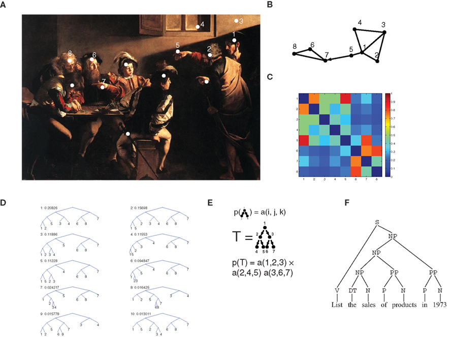
Figure 1. Relational representation of episodes and stochastic context-free grammars for semantic memory. (A) In this episode, taken from the painting “The calling of Matthew” by Caravaggio (1571–1610) a biblical episode is portrayed: Jesus (to the right, number 1) enters a room, and points to Matthew (6) who makes a hand gesture (7) responding in surprise. The white dots indicate some of the main items in the scene. (B) A graph representation of the interrelationships between the items [numbers in (A)] as they can be deduced from the scene: items with a stronger association are displayed as closer to each other. The arrow indicates an association with a strong directional character (Matthew gesture – 7 – is in response, and temporally following Jesus’ gesture – 5). (C) Color-coded matrix representation of the associations displayed in (B). Note that the matrix elements are not necessarily symmetric, in particular, the (5,7) element is larger than the (7,5) element, because of the directional relationship described in (B). (D) Hierarchical clustering derived from the episodic association matrix of (C) (see Section 2). The 10 most likely trees are displayed, each with its assigned probability. (E) Scheme of a branching process: the 3-D matrix a(i,j,k) denotes the probability that node i may generate nodes j and k. The probability of a complete tree is the product of transition probability at all nodes. (F) Parsing tree of an English sentence: non-terminal nodes denote syntactic and grammatical components of the sentence (NP, noun phrase; PP, prepositional phrase; V, verb; N, noun; S, “sentence” or “start” node, at the root of the tree).

The activity of hippocampal neurons is well-suited to implement this relational code: During wakefulness, each entity (for example, each location) will elicit the activity of a cell assembly (a coherent group of cells), with the probability for co-activation of two cell assemblies as an increasing function of the association between the two encoded entities (McNaughton and Morris, 1987). Thus, associational strength in the sense proposed here can be carried by coherent cell activity. For hippocampal place cells, for example, cells with overlapping place fields will have highly correlated activities. During sleep, the same activity correlations are reactivated (Wilson and McNaughton, 1994).

It is tempting to speculate that episodic association matrices for several episodes can be stored by linear superimposition in the synaptic matrix of an auto-associative attractor network, as assumed in the Hopfield model (Hopfield, 1982). In this way, episodes could be retrieved by pattern completion upon presentation of incomplete cues, and spontaneously activated (or replayed) independently. This has been suggested as a useful model of episodic memory (McNaughton and Morris, 1987; McClelland et al., 1995; Shen and McNaughton, 1996) and a candidate description of the function of the hippocampus, particularly with respect to subfield CA3, and its rich recurrent connectivity (Treves and Rolls, 1994). Here, however, we will not model the dynamics of episodic memory explicitly, and we will just assume that the episodic module is capable of storing and retrieving these relational data.

As we will see below, the hierarchical clustering operation may be performed by activity initiated by hippocampal reactivation, and propagated through several stages of cortical modules. It will be taken as the starting point for the training of semantic memory.

2.2 Stochastic Grammars for Semantic Memory

Semantic memory extracts regularities manifesting themselves in multiple distinct episodes (Quillian, 1968; Rogers and McClelland, 2004). In our framework, semantic memory is seen as a generative model of the world, based on the accumulation of experience. In Bayesian statistics, a generative model is a prescription to produce a probability for each possible episode, based on the previously acquired corpus of knowledge. The model can then be inverted using Bayes’ rule, to produce interpretations of further data. The model will assign a large probability to a likely episode (regardless of whether that particular episode was observed before), and smaller probabilities to episodes that do not fit the model’s current experience of the world. Once the model has been trained on the acquired experience, the values of its parameters can be seen as a statistical description of regularities in the world, potentially of a very complex nature. After training, Bayesian inference can be used to analyze further episodes, to assess its most likely “causes,” or underlying relationships. If only partial evidence is available, Bayesian inference will also support pattern completion.

Simple models for semantic memory and consolidation (McClelland et al., 1995; Kali and Dayan, 2004), have defined semantic knowledge in terms of pairwise associations between items. In fact, pairwise association can already provide rich representations of episodes, which can be embedded in a semantic system. For example, in Figure 1A, associating Jesus (1) and his hand (5) depends on having a model of the human body, while coupling Jesus’ and Matthew’s gesture require Theory of Mind, and related models of gesture meaning. These complex cognitive operations, which require specific and extremely sophisticated models, well out of this work’s scope, provide an input to the episodic memory module that we summarize here in a pairwise association matrix. Thus, we would like to formulate a generative model that assigns probabilities to each possible association matrix, and capable of capturing the highly structured and complex statistical regularities in the real world. We propose here a first step in this direction borrowing from Computational linguistics. This field has devised sophisticated generative models in the form of stochastic grammars (Manning and Schütze, 1999), targeted at the analysis of language. For each sentence, stochastic grammars generate parse trees and assign to each a probability (Figure 1F). Parse trees are hierarchical groupings of sentence elements, where each group of words corresponds to a certain grammatical element. The resulting trees have terminal nodes, corresponding to the words in the sentence, and non-terminal nodes, which correspond to non-observed sentence constituents. A non-terminal node will encode, for example, the probability that a prepositional phrase (PP) is made up of a preposition (P: “of”) and a noun (N: “products”). These stochastic grammars can be trained (i.e., their parameters can be tuned) on a corpus of experienced utterances, in a supervised or unsupervised fashion.

The attractiveness of stochastic grammars is not limited to the linguistic realm (Bod, 2002); to demonstrate how they can model semantic memory, and memory consolidation phenomena, we take into consideration a particular class of grammars, termed SCFG. In SCFGs, sentences are generated by a branching process, a stochastic process in which at each stage, a state i generates two further states, j and k with probability given by the transition matrix p(i → j, k) = a(i, j, k) (Figure 1E). The process always starts from the start node S, and, in several stages, it produces a binary tree, with the words in the sentence generated as the terminal leaves of the tree, and the syntactical components of the sentence as non-terminal nodes. To this tree, a probability is assigned which is the product of the transition probabilities at each non-terminal node. Thus, a(i,j,k) represents all of the knowledge embedded in the grammar, that is all grammatical rules. Such knowledge can be extracted from a body of experienced sentences, through EM algorithms such as the inside–outside algorithm (Lari and Young, 1990). This algorithm exploits a property of branching processes similar to the key property of Markov chains: if a tree is split at any given non-terminal node, the probability of the two sub-trees are independent, conditional on the identity of the node where the tree was split (Figure 2A). Because of this, probabilities can be computed from two independent terms, the first, the inside probability e(i,K), representing the probability that a certain non-terminal node i in the tree generates exactly the substring K (Figure 2B). The other term, the outside probability f(i,K), represents the probability that the non-terminal node i is generated in the process together with the complete sentence S minus the substring K. In the Expectation step (E-step) of the algorithm, the inside and outside probabilities are computed recursively (see Section 2.8.1) based on the current values of the transition matrix a(i,j,k) as computed from previous experience. The recursive algorithm highlights the respective contributions of bottom-up and top-down influences in determining these probabilities. In the maximization step (M-step), the a matrix is updated based on the value of the inside and outside probabilities.

FIGURE 2

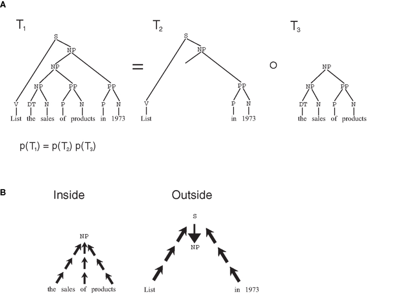
Figure 2. Inside–outside algorithm. (A) Markov-like property for trees in branching processes: if a tree T₁ is split in two sub-trees T₂ and T₃, the probability of the original tree is the product of the probabilities of the two sub-trees. Also, the two sub-trees are independent conditional to the value of the node at the separation point. (B) The probabilities in the two sub-trees can be computed separately: the inside probability can be computed recursively in a bottom-up fashion, the outside probabilities can be computed recursively top-down.

Thus, while trees are not the most general graph structure found in semantic data (Kemp and Tenenbaum, 2008), they provide an especially simple and efficient way to implement learning (other graphical models, especially those containing loops, do not enjoy the same Markov-like properties, making EM approaches much more difficult), and thus are a suitable starting point for an investigation of memory processes for structured information. However, in order to make use of the set of tools from computational linguistics, we need to make a key modification: Stochastic grammars are generative models for sequences of symbols, or utterances. This has to be extended to more general structures, and here we propose how to define a SCFG that generates episodes in terms of association matrices. We want to use the relational data contained in the s matrix coding observed episodes to optimize the a(i,j,k) transition matrix. We wish to obtain a grammar that, on average, assigns large probabilities to the trees where pairs of items expected, based on experience, to have large associational strengths are closely clustered. This should hold for the data the grammar is trained on, but must also allow generalization to further data. For these reasons, we change the transition rule in the branching process as follows:

$p(i\to j,k)=a(i,j,k)M(\mathbf{\text{P}},\mathbf{\text{Q}}),$(1)

that is, the probability of node i generating nodes j and k is given by the a matrix (which we will call henceforth the semantic transition matrix, and reflects accumulated knowledge), multiplied by the set-wise association M(P,Q), a function of the current episode only, measuring the associational strengths between the subset P and Q, which in the tree are generated, respectively, by nodes j and k. Such an arrangement amplifies the contributions from pairs of sets that correspond to likely entities, which may be joined together. The term M(P,Q) is obtained from the episodic association matrix s(i,j) by means of a hierarchical clustering algorithm, and denotes the likelihood that a naive observer will single out the subsets P and Q when observing all the items in P ∪ Q and their interrelationships (see Section 2.5). Eq. 1 is the key component of a generative model, defining the probabilities of episodes, both in terms of their composition (the O⁽ⁿ⁾) and the association matrix s, through the M(P,Q) function, as explained in Section 2.5.

With respect to the standard formulation of an SCFG (see, e.g., Lari and Young, 1990; Manning and Schütze, 1999) we made the further modification of eliminating the distinction between non-terminals and terminals, with unary transition probabilities between these two sorts of items. This further prescription is needed in linguistics, for example in order to categorize all nouns under a common type “noun,” but does not have an impact in the cases we will consider here. This abstract formulation has a possible parallel in cortical anatomy and physiology: for example, nodes at different levels in the parsing tree may correspond to modules at different levels in a cortical hierarchy (Felleman and Van Essen, 1991), which could be implemented in more or less distributed modules, as described below. Training such a model may require a long time: The E-step entails computing a sum over a combinatorially large number of possible parse trees, as explained in Section 2.8. A crucial assumption here is that, in the brain, this calculation is performed by Monte-Carlo sampling: this may take place during the extended memory consolidation intervals following acquisition. Eq. 25 (see Section 2.9) defines an update rule allowing gradual optimization of the a matrix through successive presentations of the episodes. In the brain this could be implemented during sleep replay as follows: during each reactivation event (corresponding, e.g., to a hippocampal sharp wave, Kudrimoti et al., 1999), a subset of the encoded episode is reactivated in the hippocampus. The probability of the representations of two entities both being active in a reactivation event is a function of their episodic associational strength (Wilson and McNaughton, 1994). The hippocampal input activates representations at multiple levels in the cortical hierarchy, corresponding to different levels in the parsing trees. At each level, the information relative to the episodic association matrix s (as well as M) can be computed from the probability that ascending inputs activate the corresponding units, so that perceptual data “percolate” in the cortical hierarchy.

2.3 Semantic Networks, Monte-Carlo Sampling, and Cortical Circuitry

Optimizing the a matrix is a very complex task, requiring the evaluation of several global quantities. However, it is possible to implement this optimization in an algorithm based on single module-based quantities, and with a dynamics inspired by the physiology of the sleeping neocortex. The learning rule in the consolidation algorithm acts on the node transition probabilities (see Section 2.9):

$\Delta a(i,j,k)\sim \frac{\eta }{E\left({\mathbf{\text{O}}}^{(n)}\right)}\left[{\Gamma }_{ijk}a(i,j,k)-{\Gamma }_i{a}^2(i,j,k)\right]$(2)

where η is the learning rate. E(O⁽ⁿ⁾), Γ_i and Γ_ijk are probability terms entering the Bayes formula (see Section 2.8.2): E(O⁽ⁿ⁾) can be interpreted as the degree of familiarity of the episode O⁽ⁿ⁾ given the current state of the model G (see Section 2.12). Moreover,

${\Gamma }_i=p\left(\text{node\hspace{0.17em}}i\text{\hspace{0.17em}is\hspace{0.17em}used},s\Rightarrow {\mathbf{\text{O}}}^{(n)}|G\right)$

and

${\Gamma }_{ijk}=p\left(i\Rightarrow j,k,\text{node\hspace{0.17em}}i\text{\hspace{0.17em}is\hspace{0.17em}used},s\Rightarrow {\mathbf{\text{O}}}^{(n)}|G\right)$

(see Section 2.8.2 for a complete derivation). Thus Γ_i is the probability that node i enters the parsing tree somewhere, and that the tree’s terminal nodes coincide with the items in the episode. Γ_ijk is the probability that node i enters the tree and spawns nodes j and k, while generating the entire episode O⁽ⁿ⁾ as the terminals in the tree. These terms can be computed recursively through the inside–outside probabilities, which are very convenient for computer calculations. However, these terms can also be directly computed as a sum of probabilities over trees

${\Gamma }_i={\displaystyle \sum _{t\in \text{trees\hspace{0.17em}including\hspace{0.17em}node\hspace{0.17em}}i}p(t)}$(3)

and

${\Gamma }_{ijk}={\displaystyle \sum _{t\in \text{trees\hspace{0.17em}including\hspace{0.17em}node\hspace{0.17em}}i\text{\hspace{0.17em}and\hspace{0.17em}}i\to j,k}p(t)}$(4)

where for each tree t the probability p(t) may be computed as a product of the transition probabilities from Eq. 1 at all nodes. Using Eqs 3 and 4 in a computer simulation may be very inefficient. However, cortical circuitries may well perform these computations during sleep replay. To see this, let us write p(t) from Eqs 36 and 37 as the product

$p(t)=E(t)Y(t)$(5)

where

$E(t)={\displaystyle \prod _j{e}^{\beta s(\mathbf{\text{P}},\mathbf{\text{Q}})}}$(6)

where the product index j runs over all non-terminal nodes in tree t and P and Q are the subsets of terminal nodes (episode items) indirectly generated by the two children of node j. s(P,Q) is a simply the average association strength between all items in P and all items in Q. Similarly,

$Y(t)={\displaystyle \prod _{j}a\left(j,c_1(j),c_2(j)\right)}$(7)

where c₁(j) and c₂(j) are the children of node j in tree t. Thus, E(t) depends only on the episodic transition strengths s. For this reason, we will name it the episodic strength of tree t. Likewise, Y(t) depends only on the semantic transition matrix a. Therefore we will call it the semantic strength of tree t. These quantities may have a neural interpretation: the semantic network (i.e., the neocortex) can be seen as a set of repeated modules, which may correspond for example to a cortical column. Each of these modules is composed of an input layer consisting of coincidence detectors (corresponding to single cells or cell groups), each triggered by the co-activation of a pair of inputs (Figure 3A). This layer projects to an output layer, which can propagate activity to downstream modules, via a set of plastic connections, which represent the transition probabilities a(i,j,k). These modules are organized in a multi-layer hierarchy, in which each module sends inputs to all modules higher up (Figure 3B), and reflecting sites spanning the entire cerebral cortex. At the base of this hierarchy sits the storage module for episodic memory, the hippocampus.

FIGURE 3

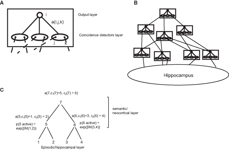
Figure 3. Possible implementation of the model in the brain. (A) A cortical module (roughly corresponding to a column), composed by a coincidence detection layer and an output layer, with modifiable connections between them. (B) A hierarchy of such modules, with the hippocampus at the bottom of the hierarchy. (C) Scheme of activation probabilities and amplitudes for a parsing tree.

These theoretical assumptions find possible counterparts in experimental data: from the dynamic point of view, hippocampal sharp waves may loosely correspond to reactivation events (Kudrimoti et al., 1999). At each event, hippocampal cell assemblies, one for items 1–4 in the episode of Figure 3C, are activated randomly, and activities propagate in the cortical hierarchy. At each cortical node, the probability of activating a coincidence detector is an increasing function of the probability of co-activation of the two groups of hippocampal units sending, through multiple layers, input to the two sides of the detector. Thus, the factors e^{βs(P, Q)} making up E(t) can be approximately computed at each level in the hierarchy. In the rat hippocampus, for example, this co-activation probability during sleep contains information about co-activations expressed during experience acquisition (Wilson and McNaughton, 1994), so that it may carry the episodic association signal defined in our theory. The activation of each cortical module will be determined by the timing of its afferent inputs. Let us assume that module 5 is activated by inputs 1 and 2 and module 6 by inputs 3 and 4. Then, a downstream module 7, receiving inputs from modules 5 and 6 will be in the position of computing the probability of co-activation of the two sets of hippocampal units (1,2) and (3,4). In this way, all terms of the form e^{βs(P, Q)} entering Eq. 6 may be computed. Across multiple reactivation events, this neural dynamics is thus equivalent to a Monte-Carlo sampling of the semantic transition probabilities through the semantic strength (Eq. 7) with a probability distribution given by the episodic strength E(t), ultimately yielding an estimate of the tree probability p(t), through Eq. 5. If a tree is activated by a reactivation event, the activity level in the units making up the tree is given by the semantic strengths (Eq. 7). This amplitude is a product of transition probabilities at all nodes in the trees. For each tree activation, this can be computed, in a bottom-up fashion, at the start node (the most downstream node in the hierarchy). It may then be communicated to lower nodes by top-down feedback connections, from higher-order (frontal) cortical areas to lower order sensory, upstream areas, reflecting top-down influences from frontal cortices. Eq. 2 has a further E(O⁽ⁿ⁾) term in the denominator, which lends itself to an interesting interpretation: this term is proportional to the general familiarity of the current episode (see Section 2.12). Thus, plasticity is suppressed for familiar episodes, and enhanced for novel ones, which have a larger impact on learning. This type of filtering is similar to the role assigned to cholinergic neuromodulation by theories of novelty-based gating of learning (Yu and Dayan, 2005). It is interesting to note that the term E(O⁽ⁿ⁾) is computed at the top of the tree, which in a cortical hierarchy would correspond to the prefrontal cortex, harboring the cortical areas which exert the strongest control over neuromodulatory structures (Mesulam and Mufson, 1984; Zaborszky et al., 1997), and have been implicated in novelty assessment (see, e.g., Ljungberg et al., 1992).

Last, connections representing the semantic transition matrix are modified according to the rule of Eq. 2: at each reactivation event, only synapses in cortical modules recruited in the activated tree are modified. The two terms on the right hand side of Eq. 2 can be seen as giving rise to two plasticity processes: connections from the activated coincidence detector to the output layer are incremented by a factor ηY(t)a(i, j, k) (analogous to long-term potentiation), and synapses from all coincident detectors to the module’s output layer are decreased by a factor ηY(T)(a(i, j, k))², similar to long-term depression.

2.4 Definitions and Notation

Data are supplied to the model as a sequence of distinct observations or episodes, with the n-th episode characterized by a set of N observed objects ${\mathbf{\text{O}}}^{(n)}\equiv \{o_1^{(n)},\dots ,o_N^{(n)}\},$ which constitute the terminal nodes of the parsing tree, and by an episodic association matrix $s_{ij}^{(n)},$ $0\le s_{ij}^{(n)}\le 1,\forall i,j,n$ (the superscript n will be dropped whenever evident from context), which reflects the degree of associations between pairs of objects as they are perceived in that particular observation. The s⁽ⁿ⁾ matrix is supposed to be computed and stored in the episodic memory module; it encodes, for example, spatial and temporal proximity. Temporal ordering can be embedded in the representation by assuming that $s_{ij}^{(n)}\ne s_{ji}^{(n)}.$ By convention, if $o_i^{(n)}$ temporally follows $o_j^{(n)},$ then $s_{ij}^{(n)}>s_{ji}^{(n)}.$ Because the representation of each object has already been processed by the semantic modules at the moment of perception, the episodic association matrix will also reflect, indirectly, associational biases already present in the cortex.

We will say that subset K ⊂ O⁽ⁿ⁾ is generated in a parse tree if all and only the observables o ∈ K are the leaves of one of its sub-trees. Each parse tree will be assigned a probability equal to the product of the probability of each node. The probability of each node (say, a node in which node i generates, as children, nodes j and k) will be in turn, the product of two terms (Eq. 1): one, originating from the episodic information, reflecting the episodic association between the subsets P and Q, generated in the parse, respectively, by nodes j and k. This will be given by the function M(P,Q), defined below. This term represents a major difference with respect to the original definition of SCFGs. The second term comes from the semantic module, and, like in a regular SCFG, reflects the probability that the two nodes j, k are generated by the parent i, given that parent i is used in the parsing. This latter probability represents the model’s “belief” about the underlying causes of the current episode, and the consequent parsing. This is given by the semantic transition matrix a(i,j,k), which is learned from experience as explained in the next section.

2.5 Calculation of Set-Wise Association M⁽ⁿ⁾(P, Q)

In order to extract categories and concepts from an episode at all orders of complexity, it is necessary to evaluate the episodic associations not only between pairs of single items, but also between pairs of item subsets I and J (each subset potentially corresponding to a higher-order concept). We term the matrix containing such associations M⁽ⁿ⁾. This matrix may be defined by means of a pairwise hierarchical clustering, based on the episodic association between terminal nodes for I, J ⊂ O⁽ⁿ⁾, I ∩ J = ø

$M^{(n)}(\mathbf{\text{I}},\mathbf{\text{J}})=p(\mathbf{\text{I}}\cup \text{J\hspace{0.17em}is\hspace{0.17em}split\hspace{0.17em}into\hspace{0.17em}I},\mathbf{\text{J}})$(8)

Thus, M⁽ⁿ⁾(I, J) quantifies the probability of recognizing I and J as coherent entities, when all the items in I ∪ J are presented. M⁽ⁿ⁾(I, J) may be generated as follows.

1. For the n-th episode, generate the set T⁰(O⁽ⁿ⁾) of all possible binary trees with $o_1^{(n)},\dots ,o_N^{(n)}$ as the (ordered) labeled terminal nodes. In a computer simulation this can be done by following the procedure devised by Rohlf (1983), augmented to generate all possible orderings of nodes.

2. For each tree t ∈ T⁰(O⁽ⁿ⁾), compute a global episodic association strength S(t) with the following algorithm

(a) set S(t) = 1

(b) for each terminal node $o_i^{(n)}$, set $L(o_i^{(n)})=\left\{o_i^{(n)}\right\}$ (the set only composed by the element $o_i^{(n)}$), where the function L(i) denotes the set of terminals generated by the node i in tree t

(c) find the bottom-left-most node n which has two leaves p and q as children, eliminate p and q and substitute n with new terminal node z

(d) set $S(t)=S(t)\cdot e^{\beta s_{pq}}$

(e) set L(z) = L(p) ∪ L(q)

(f) generate the associations between z and all other terminal nodes i with the formula

$s_{iz}=s\left(L(i),L(j)\right),$

where $s(\mathbf{\text{P}},\mathbf{\text{Q}})=\frac{1}{\#\mathbf{\text{P}}\#\mathbf{\text{Q}}}{\sum }_{m\in \mathbf{\text{P}},n\in \mathbf{\text{Q}}}{s}_{mn},$ and #P is the cardinality of P.

(g) go back to (c) until there is a single node

It is easy to demonstrate the following important

Property: Let t ∈ T⁰(O⁽ⁿ⁾), that is, one of the trees that generate O⁽ⁿ⁾. Let u and v be two sub-trees such that t = u°v (that is, t is composed by substituting the root of v to a terminal node i of u). Let V be such that v ∈ T⁰(V) and u ∈ T¹(O⁽ⁿ⁾\V), that is the set of all sub-trees having the elements of O⁽ⁿ⁾\V, plus one extra “free” node i as terminals. Then

$S(t)=S(u)S(v)e^{-\beta s\left(\mathbf{\text{v}},{\mathbf{\text{o}}}^{(n)}\backslash \mathbf{\text{v}}\right)}$(9)

3. set the observational probability of tree T based on the prescription:

$PT=\frac{S(t)}{{\displaystyle {\sum }_{t^{\prime }\in T^0\left({\mathbf{\text{O}}}^{(n)}\right)}S(t^{\prime })}}$(10)

4. set

$M(\mathbf{\text{P}},\mathbf{\text{Q}})=\frac{{\displaystyle {\sum }_{t\in T^0(\mathbf{\text{P}},\mathbf{\text{Q}})}S(t)}}{{\displaystyle {\sum }_{t\in T^0(\mathbf{\text{P}}\cup \mathbf{\text{Q}})}S(t)}},$(11)

where T(P,Q) is the set of all trees in which P ∪ Q is split into P and Q.

M(P,Q) can be interpreted as the probability that an observer having only access to the episodic information would split the set P ∪ Q into P and Q. Note how the parameter β performs a “softmax” operation of sorts: a large value of β will concentrate all the probability weight on the most probable tree, a lower value will distribute the weight more evenly.

2.6 Asymmetric Associations

In order to encode temporal order, it is necessary to have asymmetric associations strengths s_ij. We have chosen here the form (Figure 6B):

$s_{ij}=\{\begin{array}{ll}{e}^{-{\lambda }_1\left(t(i)-t(j)\right)}\hfill & t(i)>t(j)\hfill \\ e^{-{\lambda }_2\left(t(j)-t(i)\right)}\hfill & t(i)<t(j)\hfill \end{array},$(12)

where t(i) is the time of occurrence of item i. In the simulations for Figures 6 and 7, λ₁ = 5 and λ₂ = 1.5 were used, ensuring that associations were larger from preceding to subsequent items than vice versa.

2.7 Full Generative Model

The branching process (Eq. 1) gives a prescription on how to generate episodes. The association matrix enters the transition probabilities only trough the M(P,Q) functions. Thus the generative model can be expressed as follows:

1. generate a parsing tree t with probability

${\mathbf{\text{P}}}_{tree}(t)={\displaystyle \prod _{i\in NT(t)}a\left(i,c_1(i,t),c_2(i,t)\right)}$

where NT(t) is the set of nodes in tree t, c_1,2(i, t) are the two children of node i.

2. draw the association matrix Sⁿ according to the distribution

${\mathbf{\text{P}}}_{assoc}\left(S^n\right)=\frac{1}{\mathbf{\text{Z}}}{\displaystyle \prod _{i\in NT(t)}M\left(\mathbf{\text{C}}\left(c_1(i,t)\right),\mathbf{\text{C}}\left(c_2(i,t)\right)\right)}.$

where C(i) is the subset of the episode spanned by the node i, and the constant Z ensures normalization of P_assoc.

2.8 Generalized Inside–Outside Algorithm for Extraction of Semantic Information

The extraction of the semantic transition matrix a(i,j,k) from experience is performed by means of a generalized inside–outside algorithm (Lari and Young, 1990). Inside–outside is the branching process equivalent to the forward-backward algorithm used to train Hidden Markov Models (Rabiner, 1989). The main difference between the algorithm presented here and the algorithm by Lari and Young (1990) is the fact that here we deal with data in which interrelationships are more complex than what may be captured by sequential ordering. Rather, we need to rely on the associations encoded by the episodic module to figure out which nodes can be parsed as siblings.

Similarly to Lari and Young (1990), we assume that each episode O⁽ⁿ⁾ is generated by a tree having as root the start symbol S.

In SCFGs the matrix a(i,j,k) is defined as:

$a(i,j,k)=p(i\to j,k|i\text{\hspace{0.17em}is\hspace{0.17em}used\hspace{0.17em}in\hspace{0.17em}the\hspace{0.17em}parse\hspace{0.17em}tree})$(13)

with

${\displaystyle \sum _{j,k}a(i,j,k)=1\forall i}$(14)

We modified this rule, according to Eq. 1:

$p(i\to j,k)=a(i,j,k)M(\mathbf{\text{P}},\mathbf{\text{Q}}),$

where P and Q are the sets of terminals descending from i and j respectively. The matrix a represents the generative model of the world constituting the semantic memory, and we will indicate it by the letter G.

2.8.1 The E-step

In the E-step of an EM algorithm, the probabilities of the observed data are evaluated based on the current value of the hidden parameters in the model, in this case the a(i,j,k) matrix. To do so, the generalized inside–outside algorithm defines the inside probabilities (Figure 2B), for the n-th episode:

$\begin{array}{c}{e}^{(n)}(i,\mathbf{\text{P}})=\mathbf{\text{P}}(i\Rightarrow \mathbf{\text{P}}|G)\\ ={\displaystyle \sum _{j,k}{\displaystyle \sum _{\mathbf{\text{Q}}\subset \mathbf{\text{P}}}a(i,j,k)M^{(n)}(\mathbf{\text{Q}},\mathbf{\text{P}}\backslash \mathbf{\text{Q}})e(j,\mathbf{\text{Q}})e(k,\mathbf{\text{P}}\backslash \mathbf{\text{Q}})}}.\end{array}$(15)

For sets P of cardinality 1:

$\begin{array}{l}e\left(i,\left\{i\right\}\right)=1\\ e(i,\mathbf{\text{P}})=0\text{\hspace{1em}P}\ne \left\{i\right\}\forall i\end{array}$(16)

e(i,P) is the probability that i generates the subset P of the episode O⁽ⁿ⁾. Note that the e(i,P) can be computed recursively in a “bottom-up” fashion, from the inside probabilities for the subsets of P through Eq. 15, with the starting condition in Eq. 16.

The outside probabilities f(i,P,) are defined as:

$\begin{array}{c}f(i,\mathbf{\text{P}})=P\left(S\Rightarrow \left({\mathbf{\text{O}}}^{(n)}\backslash \mathbf{\text{P}}\right)\cup i|G\right)\\ ={\displaystyle \sum _{j,k}{\displaystyle \sum _{\text{Q:P}\subset \mathbf{\text{Q}}\subseteq {\mathbf{\text{Q}}}^{(n)}}(a(j,k,i)M^{(n)}(\mathbf{\text{P}},\mathbf{\text{Q}}\backslash \mathbf{\text{P}})f(j,\mathbf{\text{Q}})e(k,\mathbf{\text{Q}}\backslash \mathbf{\text{P}})}}\\ +a(j,i,k)M^{(n)}(\mathbf{\text{Q}}\backslash \mathbf{\text{P}},\mathbf{\text{P}})f(j,\mathbf{\text{Q}})e(k,\mathbf{\text{Q}}\backslash \mathbf{\text{P}}))\end{array}$(17)

with the condition

$f\left(S,{\mathbf{\text{O}}}^{(n)}\right)=1$(18)

where S is the start symbol that will be at the root of all parse trees. f(i,P) are the probabilities that the start symbol S generates everything but the set P, plus the symbol i (Figure 2B). Note that, once the inside probabilities are computed, the outside probabilities can be computed recursively “top-down” from the outside probabilities for supersets of P, with the starting condition in Eq. 18.

2.8.2 The M-step

Once the e and f probabilities are computed, the M-step, that is, the optimization of the semantic probabilities a(i,j,k) can be performed as follows.

First, note that

$\begin{array}{c}e(i,\mathbf{\text{P}})f(i,\mathbf{\text{P}})=p\left(S\Rightarrow {\mathbf{\text{O}}}^{(n)},i\Rightarrow \mathbf{\text{P}}|G\right)\\ =p\left(S\Rightarrow {\mathbf{\text{O}}}^{(n)}\right)p\left(i\Rightarrow \mathbf{\text{P}}|S\Rightarrow {\mathbf{\text{O}}}^{(n)},G\right)\end{array}$(19)

Let E(O⁽ⁿ⁾) = P(s → O⁽ⁿ⁾|G) = e(S, O⁽ⁿ⁾)

We have

$\begin{array}{r}{\Gamma }_i({\mathbf{\text{O}}}^{(n)},G)=p\left(i\text{\hspace{0.17em}is\hspace{0.17em}used\hspace{0.17em}in\hspace{0.17em}the\hspace{0.17em}parse},S\Rightarrow {\mathbf{\text{O}}}^{(n)}|G\right)\\ ={\displaystyle \sum _{\mathbf{\text{P}}}e(i,\mathbf{\text{P}})f(i,\mathbf{\text{P}})}\\ ={\displaystyle \sum _{j,k}{\displaystyle \sum _{\mathbf{\text{P}}}{\displaystyle \sum _{\mathbf{\text{Q}}\subset \mathbf{\text{P}}}a(i,j,k)e(j,\mathbf{\text{Q}})e(k,\mathbf{\text{P}}\backslash \mathbf{\text{Q}})M(\mathbf{\text{Q}},\mathbf{\text{P}}\backslash \mathbf{\text{Q}})f(i,\mathbf{\text{P}})}}}\end{array}$(20)

and

$\begin{array}{c}{\Gamma }_{ijk}\left({\mathbf{\text{O}}}^{(n)},G\right)=\mathbf{\text{P}}\left(i\Rightarrow j,k,i\text{\hspace{0.17em}is\hspace{0.17em}used},S\Rightarrow {\mathbf{\text{O}}}^{(n)}|G\right)\\ ={\displaystyle \sum _{\mathbf{\text{P}}}{\displaystyle \sum _{\mathbf{\text{Q}}\subset \mathbf{\text{P}}}a(i,j,k)e(j,\mathbf{\text{Q}})e(k,\mathbf{\text{P}}\backslash \mathbf{\text{Q}})M(\mathbf{\text{Q}},\mathbf{\text{P}}\backslash \mathbf{\text{Q}})f(i,\mathbf{\text{P}})}}\end{array}$(21)

and then, by the Bayes rule:

$\begin{array}{c}a(i,j,k)=p\left(i\Rightarrow j,k|i\text{\hspace{0.17em}is\hspace{0.17em}used},S\Rightarrow {\mathbf{\text{O}}}^{(n)},G\right)\\ =\frac{p(i\to j,k,i\text{\hspace{0.17em}is\hspace{0.17em}used})}{p(i\text{\hspace{0.17em}is\hspace{0.17em}used})}=\frac{{\Gamma }_{ijk}\left({\mathbf{\text{O}}}^{(n)},G\right)}{{\Gamma }_i\left({\mathbf{\text{O}}}^{(n)},G\right)}.\end{array}$(22)

Following Lari and Young (1990) if there are N episodes that are memorized, a(i,j,k) can be computed as:

$a(i,j,k)=\frac{{\displaystyle {\sum }_n{\Gamma }_{ijk}\left({\mathbf{\text{O}}}^{(n)}\right)}}{{\displaystyle {\sum }_n{\Gamma }_i\left({\mathbf{\text{O}}}^{(n)}\right)}}$(23)

where each term in the sum refers to one of the episodes.

2.9 Online Learning

The previous sections show how an iterative EM algorithm can be defined: first, the semantic transition matrix is randomly initialized, then, in the E-step, the inside probabilities are first computed bottom-up with Eq. 15, from the data and the current value of a(i,j,k), then the outside probabilities are computed top-down with Eq. 17. In the M-step the a matrix is re-evaluated by means of Eq. 22. Optimization takes place by multiple EM iterations. These equations, however, presuppose batch learning, that is, all episodes are available for training the model at the same time. A more flexible framework, which can more closely reproduce the way actual memories are acquired, needs to be updated incrementally, one episode at a time. An incremental form of the algorithm, as delineated by Neal and Hinton (1998), can be defined in analogy with the online update rule for Hidden Markov Models defined by Baldi and Chauvin (1994): define

$a(i,j,k)=\frac{e^{w(i,j,k)}}{{\displaystyle {\sum }_{j^{\prime },k^{\prime }}{e}^{w(i,j^{\prime },k^{\prime })}}}$(24)

which fulfills by definition the normalization constraint of Eq. 14. We now define an online update rule for the w matrix

$\Delta w(i,j,k)=\frac{\eta }{E\left({\mathbf{\text{O}}}^{(n)}\right)}\left[{\Gamma }_{ijk}-{\Gamma }_{i}a(i,j,k)\right]$(25)

or for small η:

$\Delta a(i,j,k)\sim \frac{\eta }{E\left({\mathbf{\text{O}}}^{(n)}\right)}\left[{\Gamma }_{ijk}a(i,j,k)-{\Gamma }_i{a}^2(i,j,k)\right]$(26)

where, again, η is a rate parameter controlling the speed of the learning process. In analogy to Baldi and Chauvin’s (1994) work, this rule will converge toward a (possibly local) maximum of p(O⁽ⁿ⁾, G) = p(S → O⁽ⁿ⁾|G), the likelihood of model G (completely defined by a(i,j,k) given the observation O(n). As explained in the Results section, the two terms on the right hand side of Eq. 25 may be interpreted, respectively, as homosynaptic LTP and heterosynaptic LTD.

Note the role played by E(O⁽ⁿ⁾) in the denominator of Eq. 26: when the likelihood is low, for example when a novel episode is presented, the change in w will be relatively greater than when a well-learned episode (giving the current state of the model a high likelihood) is presented. Hence, the rule privileges learning of novel information with respect to familiar episodes.

2.10 Local Form of the Learning Rule

We will show here how we can express the inside and outside probabilities, as well as the terms entering the optimization rule for the semantic transition matrix as sums and products over terms that can be computed locally at the nodes of a hierarchical neural network. This is an essential step in order to map our algorithm on a neural network model.

Let us consider first the inside probabilities: from Eq. 15 we have

$e^{(n)}(i,\mathbf{\text{P}})={\displaystyle \sum _{j,k}{\displaystyle \sum _{{\mathbf{\text{Q}}}_1\subset \mathbf{\text{P}}}a(i,j,k)M^{(n)}\left({\mathbf{\text{Q}}}_1,{\mathbf{\text{Q}}}_2\right)e\left(j,{\mathbf{\text{Q}}}_1\right)e\left(k,{\mathbf{\text{Q}}}_2\right)}},$

having defined Q₂ = P\Q₁. By making use of Eq. 11 we then obtain:

$e^{(n)}(i,\mathbf{\text{P}})=\frac{{\displaystyle {\sum }_{j,k}{\displaystyle {\sum }_{{\mathbf{\text{Q}}}_1\subset \mathbf{\text{P}}}{\displaystyle {\sum }_{t\in T\left({\mathbf{\text{Q}}}_1,{\mathbf{\text{Q}}}_2\right)}a(i,j,k)S(t)e(j,{\mathbf{\text{Q}}}_1)e(k,{\mathbf{\text{Q}}}_2)}}}}{{\displaystyle {\sum }_{t\in T(\mathbf{\text{P}})}S(t)}}$

where T(Q₁, Q₂) is the set of all trees in which set P is split in sets Q₁ and Q₂ and then, by making use of Eq. 9:

$\begin{array}{r}{e}^{\text{(}n\text{)}}\text{(}i\text{,P)}={\left({\displaystyle \sum _{t_3\in T^1(\mathbf{\text{P}})}S(t_3)e^{-\beta s\left(\mathbf{\text{P}},{\mathbf{\text{O}}}^{(n)}\backslash \mathbf{\text{P}}\right)}}{\displaystyle \sum _{t\in T^0(\mathbf{\text{P}})}S(t)}\right)}^{-1}\\ \times {\displaystyle \sum _{j,k}{\displaystyle \sum _{{\mathbf{\text{Q}}}_1\subset \mathbf{\text{P}}}a(i,j,k)}{\displaystyle \sum _{t_3\in T^1(\mathbf{\text{P}})}S(t_3)e^{-\beta s\left(\mathbf{\text{P}},{\mathbf{\text{O}}}^{(n)}\backslash \mathbf{\text{P}}\right)}{e}^{-\beta s\left({\mathbf{\text{Q}}}_1,{\mathbf{\text{Q}}}_2\right)}}}\\ \times {\displaystyle \sum _{t1\in T^0({\mathbf{\text{Q}}}_1)}S(t_1)}{\displaystyle \sum _{t1\in T^0({\mathbf{\text{Q}}}_2)}S(t_2)}.\end{array}$(27)

Here, T⁰(P) denotes the inside trees of P, i.e., the set of trees spanning the ordered subset P, and T¹(P) is the set of outside trees of P, i.e., the set of sub-trees starting from S and spanning O⁽ⁿ⁾\P, plus an extra terminal node. Let us now define the reduced inside probabilities

$\tilde{e}(i,\mathbf{\text{P}})={\displaystyle \sum _{t\in T^0(\mathbf{\text{P}})}S(t)e(i,\mathbf{\text{P}})},$(28)

we then have

$\tilde{e}(i,\mathbf{\text{P}})={\displaystyle \sum _{j,k}{\displaystyle \sum _{{\mathbf{\text{Q}}}_1\subset \mathbf{\text{P}}}a(i,j,k)e^{-\beta s\left({\mathbf{\text{Q}}}_1,{\mathbf{\text{Q}}}_2\right)}\tilde{e}(j,{\mathbf{\text{Q}}}_1)\tilde{e}(k,{\mathbf{\text{Q}}}_2)}}.$(29)

By induction we can then prove that

$\tilde{e}(i,\mathbf{\text{P}})={\displaystyle \sum _{t\in T^{0,l}(\mathbf{\text{P}},i)}{\displaystyle \prod _{j\in NT(t)}a\left(j,c_1(j),c_2(j)\right)e^{-\beta s\left(\mathbf{\text{C}}\left(c_1(j),t\right),\mathbf{\text{C}}\left(c_2(j),t\right)\right)}}},$(30)

where c₁(i), c₂(i) are the left and right children of node i in tree t (with labeled non-terminals) and C(i,t) is the subset of terminals generated by node i in tree t. NT(t) is the set of labeled non-terminals nodes of tree t. T^0,l(P,i) is the set of trees with labeled non-terminals with root labeled with i and generating P.

Similarly, for the outside probabilities, from Eq. 17:

$\begin{array}{c}f(i,\mathbf{\text{P}})={\displaystyle \sum _{j,k}{\displaystyle \sum _{\mathbf{\text{Q}}:\mathbf{\text{P}}\subset \mathbf{\text{Q}}\subseteq {\mathbf{\text{P}}}^{(n)}}(a(j,i,k)M^{(n)}\left({\mathbf{\text{P}}}_1,{\mathbf{\text{P}}}_2\right)}}\\ +a(j,k,i)M^{(n)}\left({\mathbf{\text{P}}}_2,{\mathbf{\text{P}}}_1\right))f(j,\mathbf{\text{Q}})e\left(k,{\mathbf{\text{P}}}_2\right).\end{array}$(31)

Where we assumed P₁ = P and P₂ = O⁽ⁿ⁾P.

Inserting Eq. 11 in the previous formula we obtain

$\begin{array}{l}{f}^{(n)}(i,\mathbf{\text{P}})\\ ={\displaystyle \sum _{j,k}{\displaystyle \sum _{\mathbf{\text{Q}}:\mathbf{\text{P}}\subset \mathbf{\text{Q}}\subseteq {\mathbf{\text{O}}}^{(\mathbf{\text{n}})}}\frac{1}{{\displaystyle {\sum }_{t\in T(\mathbf{\text{Q}})}S(t)}}\left({\displaystyle \sum _{t\in T\left({\mathbf{\text{P}}}_1,{\mathbf{\text{P}}}_2\right)}a(j,i,k)}+{\displaystyle \sum _{t\in T\left({\mathbf{\text{P}}}_2,{\mathbf{\text{P}}}_1\right)}a(j,k,i)}\right)}}\\ \times S(t)f(j,\mathbf{\text{Q}})e\left(k,{\mathbf{\text{P}}}_2\right).\end{array}$(32)

T(P₁, P₂) is the set of possible trees which generate Q and split it into P₁ and P₂. By the property defined in Eq. 9:

$\begin{array}{l}{f}^{(n)}(i,\mathbf{\text{P}})={\displaystyle \sum _{j,k}{\displaystyle \sum _{\mathbf{\text{Q}}:\mathbf{\text{P}}\subset \mathbf{\text{Q}}\subseteq {\mathbf{\text{O}}}^{(n)}}\frac{1}{{\displaystyle {\sum }_{t\in T(\mathbf{\text{Q}})}S(t)}}}}\\ \times {\displaystyle \sum _{t_1\in T^1(\mathbf{\text{Q}})}S\left(t_1\right)}\left(a(j,k,i)e^{-\beta s\left({\mathbf{\text{P}}}_1,{\mathbf{\text{P}}}_2\right)}+a(j,i,k)e^{-\beta s\left({\mathbf{\text{P}}}_2,{\mathbf{\text{P}}}_1\right)}\right)\\ \times {\displaystyle \sum _{t_2\in T^0\left({\mathbf{\text{P}}}_2\right)}S\left(t_2\right)e\left(k,{\mathbf{\text{P}}}_2\right)}{\displaystyle \sum _{t_3\in T^0\left({\mathbf{\text{P}}}_1\right)}f(j,\mathbf{\text{Q}})}+swap\text{.}\end{array}$

“Swap” here refers to the same terms with swapped roles for P₁ and P₂ We can define the reduced outside probabilities $\tilde{f}(i,\mathbf{\text{P}})=\frac{f(i,\mathbf{\text{P}})}{{\sum }_{t\in T^0(\mathbf{\text{P}})}S(t)}.$ Eq. 18 gives us an initialization condition for the f:

$\tilde{f}\left(S,{\mathbf{\text{O}}}^{(n)}\right)=\frac{1}{{\displaystyle {\sum }_{t\in T^0\left({\mathbf{\text{O}}}^{(\mathbf{\text{n}})}\right)}S(t)}}$(33)

We then have

$\begin{array}{l}\tilde{f}(i,\mathbf{\text{P}})\\ =\frac{1}{{\displaystyle {\sum }_{t\in T^0\left({\mathbf{\text{O}}}^{(\mathbf{\text{n}})}\right)}S(t)}}{\displaystyle \sum _{j,k}{\displaystyle \sum _{\mathbf{\text{Q}}:\mathbf{\text{P}}\subset \mathbf{\text{Q}}\subseteq {\mathbf{\text{O}}}^{(\mathbf{\text{n}})}}\left(a(j,k,i)e^{-\beta s\left({\mathbf{\text{P}}}_1,{\mathbf{\text{P}}}_2\right)}+a(j,i,k)e^{-\beta s\left({\mathbf{\text{P}}}_2,{\mathbf{\text{P}}}_1\right)}\right)}}\\ \times \tilde{e}\left(k,{\mathbf{\text{P}}}_2\right)\tilde{f}(j,\mathbf{\text{Q}})+\text{swap.}\end{array}$(34)

By induction:

$\tilde{f}(i,\mathbf{\text{P}})=\frac{1}{{\displaystyle {\sum }_{t\in T^{0(\mathbf{\text{n}})}}S(t)}}{\displaystyle \sum _{t\in T^{1,l}(\mathbf{\text{P}},i)}{\displaystyle \prod _{j\in NT(t)}a\left(j,c_1(j),c_2(j)\right)e^{-\beta s\left(\mathbf{\text{C}}\left(c_1(j),t\right),\mathbf{\text{C}}\left(c_2(j),t\right)\right)}}}$(35)

where now T^1,l(P,i) is the set of outside trees of P where the extra terminal has exactly label i. We can now express Γ_i as follows:

$\begin{array}{l}{\Gamma }_i={\displaystyle \sum _{\mathbf{\text{P}}}f(i,\mathbf{\text{P}})e(i,\mathbf{\text{P}})}\\ ={\displaystyle \sum _{\mathbf{\text{P}}}\tilde{f}(i,\mathbf{\text{P}})\tilde{e}(i,\mathbf{\text{P}})}\\ =\frac{1}{{\displaystyle {\sum }_{t\in T^{0(\mathbf{\text{n}})}}S(t)}}{\displaystyle \sum _{t\in T^l\left({\mathbf{\text{O}}}^{(\mathbf{\text{n}})},i\right)}{\displaystyle \prod _{j\in NT(t)}a\left(j,c_1(j),c_2(j)\right)e^{-\beta s\left(\mathbf{\text{C}}\left(c_1(j),t\right),\mathbf{\text{C}}\left(c_2(j),t\right)\right)}}}\end{array}$(36)

where the sum runs on the set T^l(O⁽ⁿ⁾, i) of all trees with labeled non-terminals in which one non-terminal is labeled i, and we used the fact that $\frac{1}{\mathbf{\text{P}}({\mathbf{\text{O}}}^{(n)},G)}\frac{1}{{\sum }_{t\in T^{0(n)}}S(t)}=\tilde{e}(S,{\mathbf{\text{O}}}^{(n)}).$

Also,

$\begin{array}{l}{\Gamma }_{ijk}\\ ={\displaystyle \sum _{\mathbf{\text{P}}}{\displaystyle \sum _{{\mathbf{\text{Q}}}_1\subset \mathbf{\text{P}}}a(i,j,k)e\left(j,{\mathbf{\text{Q}}}_1\right)e(k,{\mathbf{\text{Q}}}_2)M({\mathbf{\text{Q}}}_1,{\mathbf{\text{Q}}}_2)f(i,\mathbf{\text{P}})}}\\ ={\displaystyle \sum _{\mathbf{\text{P}}}{\displaystyle \sum _{{\mathbf{\text{Q}}}_1\subset \mathbf{\text{P}}}a(i,j,k)\tilde{e}\left(j,{\mathbf{\text{Q}}}_1\right)\tilde{e}(k,{\mathbf{\text{Q}}}_2)M({\mathbf{\text{Q}}}_1,{\mathbf{\text{Q}}}_2)\tilde{f}(i,\mathbf{\text{P}})}}\\ \times \frac{{\displaystyle {\sum }_{t_1\in T_0\mathbf{\text{P}}}S\left(t_1\right)}}{{\displaystyle {\sum }_{t_2\in T_0{\mathbf{\text{P}}}_1}S\left(t_2\right)}{\displaystyle {\sum }_{t_3\in T_0{\mathbf{\text{P}}}_2}S\left(t_3\right)}}\\ ={\displaystyle \sum _{\mathbf{\text{P}}}{\displaystyle \sum _{{\mathbf{\text{Q}}}_1\subset \mathbf{\text{P}}}a(i,j,k)\tilde{e}\left(j,{\mathbf{\text{Q}}}_1\right)\tilde{e}(k,{\mathbf{\text{Q}}}_2)e^{-\beta s\left({\mathbf{\text{Q}}}_1,{\mathbf{\text{Q}}}_2\right)}\tilde{f}(i,\mathbf{\text{P}})}}\\ =\frac{1}{{\displaystyle {\sum }_{t\in T^{}}S(t)}}{\displaystyle \sum _{t\in T^l\left({\mathbf{\text{O}}}^{(n)},i\to j,k\right)}{\displaystyle \prod _{j\in NT(t)}a\left(j,c_1(j),c_2(j)\right)e^{-\beta M\left(\mathbf{\text{C}}\left(c_1(j),t\right),\mathbf{\text{C}}\left(c_2(j),t\right)\right)}}}\end{array}$(37)

where T^l(O⁽ⁿ⁾, i → j, k) denotes the set of trees with labeled non-terminals in which one non-terminal is labeled i and has, as left and right children, respectively j and k. Thus Γ_i and Γ_ijk can be expressed as sums of terms locally computable at each node according to Eqs 3–7.

2.11 Optimal Parsing

After training, in order to test the performance of our semantic memory model at retrieval, it is handy to compute what the optimal parsing tree is for a given episode, given the current state of the model, that is of the a matrix. While this would be straightforward in a parallel neural network which could estimate the likelihood of all trees at the same time, it is much harder to accomplish in computer simulations. A natural definition of an optimal tree is the tree t that maximizes the tree probability

${\mathbf{\text{P}}}_{tree}(t)={\displaystyle \prod _{i\in NT(t)}a\left(i,c_{1}i,t,c_{2}i,t\right)e^{-\beta M\left(\mathbf{\text{C}}\left(c_1(j),t\right),\mathbf{\text{C}}\left(c_2(j),t\right)\right)}}$(38)

However, finding the maximum of this expression requires a search over all possible binary trees with labeled terminals and non-terminals, a huge, impractical number. Following Goodman (1996), we adopted an alternative definition of optimality, that is the tree t that maximizes the number of correctly labeled constituents, that is

$L\mathbf{\text{C}}(t)={\displaystyle \prod _{i\in NT(t)}e\left(i,\mathbf{\text{C}}(i,t)\right)f\left(i,\mathbf{\text{C}}(i,t)\right)=\mathbf{\text{P}}\left(s\Rightarrow {\mathbf{\text{O}}}^{(n)},i\Rightarrow \mathbf{\text{P}}|G\right)}$

This measure tells us how many constituents (subsets of the entire episode) are correctly labeled, that is, their elements are the terminal nodes of a subtree having the “correct” (according to the generative model) non-terminal as the root. This measure can be computed from the inside and outside probabilities (which can be computed efficiently), and can be maximized with a simple dynamic programming algorithm, as described by Goodman (1996). This procedure was used to estimate the optimal trees displayed in Figures 4C, 5C, 6D, and 8C.

FIGURE 4

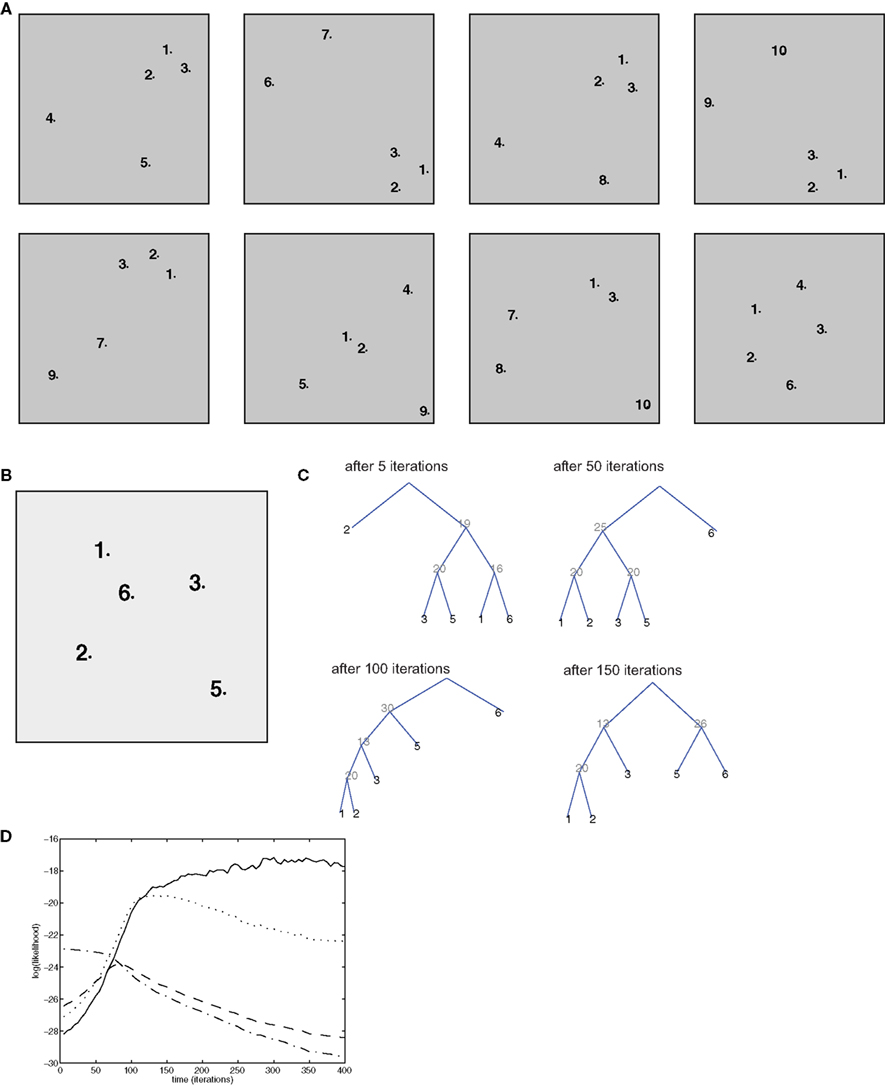
Figure 4. Simulation of bottom-up influences and decontextualization. (A) Training set, composed of 8 episodes, each composed of 5 items. (B) Test episode (not used for training). (C) Optimal parsing trees computed by the semantic model after 5, 50, 100, 150 iterations. (D) Time course of the log-likelihood of each of the parsing trees in (C): the optimal ones after 5 iteration (dash/dotted lined), 50 iterations (dashed line), 100 iterations (dotted line), 150 iterations (solid line).

FIGURE 5

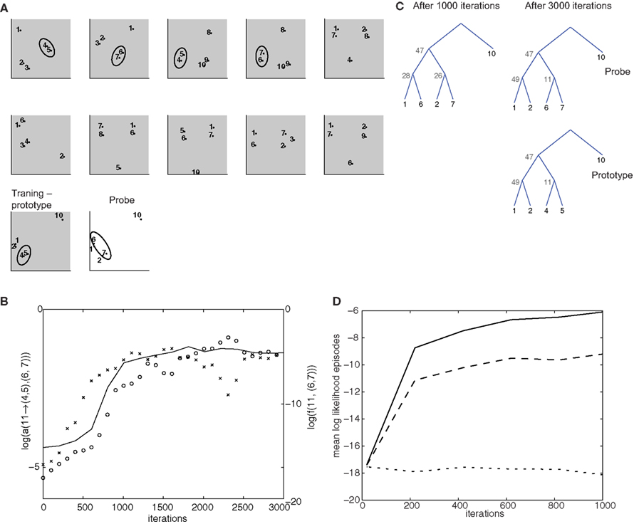
Figure 5. Simulation of top-down influences. (A) Training set, composed of 11 5-item episodes (gray background), and a “probe” episode (white background). The groups (4,5) and (6,7), which occur in the same-context in different episodes, are highlighted by the ellipses. The last training episode is termed prototype, because it contains the same items as the test episode, except for a (4,5) to (6,7) substitution. (B) Time course of log-probability of the transition elements from non-terminal node 11 to the groups (4,5) and (6,7) are indicated, respectively, by crosses and circles. The outside probability that 11 generates (6,7) in the second training episode is also shown (solid line). (C) Optimal parse trees for the test episode after 1000 and 3000 iterations and for the prototype episode after 1000 iterations. (D) Cross-validation test of potential over-fitting behavior. From the grammar model trained in the simulation for (B,C), 48 episodes were drawn. The first 40 were used for training a new grammar model for 2000 iterations. The remaining 8 were used for cross-validation. The figure shows the time of evolution average log-likelihood for the training set (solid line), the cross-validation set (dashed line) and a scrambled control set obtained by randomly shuffling the item labels from episodes drawn from the same grammar model as the previous ones.

FIGURE 6

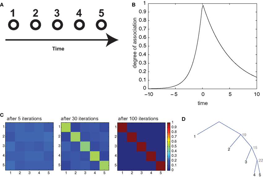
Figure 6. Serial recall of lists. (A) Episodes are composed of 5 items, in temporal sequence. (B) Temporal association as a function of temporal interval between two items. (C) Color code representation of the temporal confusion matrix after 1, 6, and 20 iterations. The confusion matrix is the probability of retrieving item X at position Y. Therefore, a diagonal matrix denotes perfect sequential recall. (D) Optimal parsing tree for the sequence after 20 iterations.

2.12 Familiarity and Episode Likelihood

Another important measure of recall is the familiarity of a newly experienced episode. In a generative model framework, this translates into the likelihood that the generative model produces that episode. By definition this corresponds to the inside probability:

$p\left({\mathbf{\text{O}}}^{(n)},G\right)=e\left(S,{\mathbf{\text{O}}}^{(n)}\right)=E\left({\mathbf{\text{O}}}^{(n)}\right),$(40)

so that familiarity can also be effectively computed. The same formula can also be used to simulate the behavior of the model in production, as for example in the simulations of Figures 6 and 7.

FIGURE 7

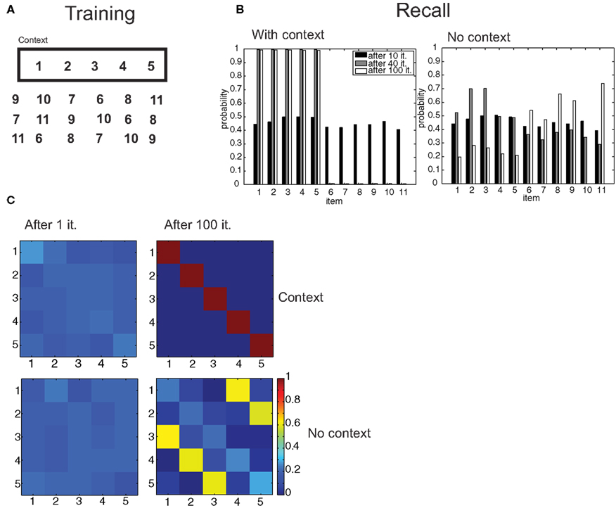
Figure 7. Free recall of lists. (A) An episode composed of the items 1–5 is learned in a certain context, other distractor episodes are learned without that context. (B) Probability of recall of items in the context and with no-context after 10, 40, and 100 iterations. (C) Confusion matrices for the (1,2,3,4,5) episode in the original context and with no-context.

2.13 Simulation Parameters

For all simulations, the parameter β was set at 3, and the learning rate η was 0.2. The number of non-terminals was 20 for the simulations of Figures 4, 6, and 7, 30 for the simulations of Figure 8, and it was 40 for the simulations in Figure 5. Each iteration consisted of two runs of the EM algorithm with the same randomly selected episode.

FIGURE 8

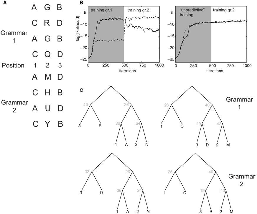
Figure 8. Learning of artificial grammars. (A) Example syllable configurations from Grammar 1 (of the form A-X-B, C-X-D) and Grammar 2 (A-X-D, C-X-B). (B) Average log-likelihood assigned by the model to examples from Grammar 1 (solid line) and 2 (dashed line) as a function of the number of training iterations. In the first 500 iterations episodes from grammar 1 (left) or the unpredictive grammar (right) are presented. (C) Optimal parse trees for Grammar 1 after 500 iterations (top) and for Grammar 2 after 1000 iterations (bottom).

3 Results

3.1 Consolidation of Bottom-Up Structures and Decontextualization

The model successfully learned complex structures present in episodic memory, and by virtue of this, it can account for several phenomena observed in memory consolidation. First, consolidated memories tend to lose their dependence on context with time, as shown for fear conditioning and socially acquired food preference (Winocur et al., 2007) and as predicted by the “transformational” theories of memory consolidation (Moscovitch et al., 2005, 2006).

Because of the properties of tree graphs, which embody the “context-free” character of SCFGs, decontextualization is obtained naturally in this model. This can be seen in simulations as follows: the model is trained on a set of 8 “episodes” (Figure 4A), each represented as a configuration of 5 items. As above, we displayed association between items as proximity in the 2-D plane. In 5 out of 8 episodes, the group of items (1, 2, 3) appears in a strongly associated form, but in 5 different contexts (different combinations of the other items completing the episode). The (1,2,3) group may represent stimuli that are closely related to each other (for example, a tone and a shock in a fear conditioning paradigm).

The consolidation algorithm is trained for 400 iterations, and in each iteration one of the training episodes, randomly chosen, is used to simulate reactivation. With time, a context-independent representation develops. To assess this, we test the resulting memory structure on a new episode (Figure 4B) which was not in the training set. In this test episode, items 1, 2, 3 appear, but the structure of the inter-items associations does not make it evident that they belong to the same group, as item 6 has in fact stronger associations with items 1, 2, and 3 than these latter have with each other. This is similar to a situation in which a distractor stimulus is interleaved between the Conditioned Stimulus (e.g., a tone) and the Unconditioned Stimulus (e.g., a shock). At the beginning of training (5 iterations), the optimal parse tree for the test episode (see Section 2.11 for definition), reflects episodic associations only (Figure 4C): in this tree, item 1 is first grouped with item 6 (the distractor), item 3 with item 5, and item 2 is isolated. Thus, the optimal parsing is completely dominated by the associations as they are perceived in that particular episode. After 50 iterations, items 1 and 2 are grouped together, after 100 iterations, items 1, 2, and 3 are grouped together in one subtree, and this is maintained after 150 iterations and afterward. The key to this behavior is the evolution of the transition probabilities for “hidden” or non-terminal nodes: with consolidation, non-terminal node 20 becomes increasingly likely to generate nodes 1 and 2, node 13 (which is the root node of the subtree encoding the (1,2,3) group) has a large probability of generating nodes 20 and 3. With time the semantic transition matrix a is shaped so that this emerging parsing (the optimal one after 150 iterations and later) remains the only one with a consistently high likelihood, with the other parsing trees becoming less and less likely (Figure 4D). Thus, nodes 13 and 20 create a higher-order representation of the “concept” of group 1, 2, 3, as they could be stored for the long-term in associational, or prefrontal cortical areas (Takashima et al., 2006). Such representation can be activated regardless of the precise context (or the remainder of the episode), and purely by bottom-up signals.

3.2 Inductive Reasoning and Top-Down Learning of Categories

While in the previous example the “inside” probabilities, that is, bottom-up processing, are critical for the outcome, much of the model’s power in complex situations arises from top-down processing. One situation in which this is visible is when different items happen to often occur in similar contexts. Then a common representation should emerge generalizing across all these items. For example, we recognize an object as a “hat,” however funny shaped it is, because we observe it on somebody’s head similar to “Bayesian model merging” (see e.g., Stolcke and Omohundro, 1994). A related cognitive task is tapped by the Advanced Progressive Matrices test of inductive reasoning (Raven et al., 1998), where a pattern has to be extracted from a number of sequential examples, and then used to complete a new examples. Performance in this task has been seen to correlate with spindle activity during slow-wave sleep (Schabus et al., 2006).

In this simulation, item groups (4,5) and (6,7) appear repeatedly interchangeably in different contexts in successive training episodes (Figure 5A). A common representation for the two groups develops, in the form of the non-terminal node 11. With training, this node sees its semantic transition probabilities to both of these groups increase (Figure 5B). As a result, the model is capable of performing inferences on configurations it has never seen before. The probe episode (Figure 5A) has the same item composition as the last training episode (“prototype”), except for group (6,7), which substitutes (4,5). Moreover, the perceptual associations do not suggest pairing 6 and 7 (rather 1 with 6 and 2 with 7). Yet, after 3000 iterations, the optimal parsing tree couples 6 and 7 through the activation of the non-terminal 11, which is driven by top-down influences (Figure 5C), in a parsing tree identical to what was computed for the prototype episode. The outside probabilities are critical for the build-up of the generalized representation: indeed, during training, the probability that 11 → (4,5) is the first to raise (Figure 5B). This leads to the increase of the top-down, outside probability f(11,(6,7)), for the episodes in which (6,7) appears en lieu of (4,5), forcing activation of node 11. Last, driven by these top-down effects, non-terminal node 11 acquires a high probability of generating (6,7) as well.

In a further simulation, we tested the generalization behavior of the model. We used the model resulting from the training on the episodes of (Figure 5A) to generate 48 episodes, and used the first 40 to train a new model, using the remaining 8 as a test set. Throughout 2000 training iterations, the log-likelihood for the training and test set rise with similar time courses, and reach levels much higher than for a shuffled control set of episodes (Figure 5D).

3.3 List Learning, Serial, and Free Recall

While not strictly a semantic memory operation, list learning is a very popular paradigm to investigate declarative memory, and has been an important benchmark for theories in the field (McClelland et al., 1995). We consider it here to assess our framework’s ability to store strictly sequential information, which is an important case for memory storage, an ability that does not follow immediately from the model’s definition. We assessed the behavior of our model in this task by considering two common experimental procedures: serial and contextual free recall. In serial recall, ordered lists are presented to the subjects, who have to recall them in the same order after a retention interval. We simulated the presentation of an ordered list by constructing an “episode” composed of 5 items (numbered from 1 to 5; Figure 6A), presented sequentially in time at regular intervals. These associations essentially reflect the temporal interval between the presentations of the respective items and they decay exponentially with that interval. To convey the notion of temporal ordering, we made the perceptual association matrix s asymmetrical, so that “backward” associations (associations from more recent to more remote items) decay more than three times faster than forward associations (Figure 6B; see Section 2). This form of association was inspired by similar patterns of confusion observed in human subjects during list retrieval (Kahana, 1996) and could find a plausible implementation in neural circuits with synapses obeying a spike-timing-dependent plasticity rule (Markram et al., 1997; Bi and Poo, 1998). We trained our model with several iterations of the consolidation algorithm described above, then, to simulate free retrieval, we used the resulting transition matrix a to compute the probabilities of “spontaneous” generation by the branching process of all permutations of the 5 items, when the episodic association matrix was set to uniform values (to mimic the absence of perceptual inputs). These probabilities are expressed in terms of a sum over all possible parsing trees having the 5 items in the target list as terminals, but can be efficiently calculated with the inside–outside algorithm (see Section 2). Then, we computed the confusion matrix C(i,j), representing the probability that item i is retrieved at the j-th position. With training, the model gradually evolved from chance-level performance to perfect serial recall (after 100 iterations; Figure 6C), indicated by a diagonal confusion matrix. This becomes possible because the optimal parsing tree (Figure 6D) as well as all of the most probable parsing trees generate the 5 items in the correct order.

In contextual free recall, subjects are shown a list of objects. After retention, they are placed in the same-context and asked to enumerate as many items in the original list as possible, regardless of their order. We simulated the training conditions by composing a target episode from a 5-item ordered list, with associations as described in Figures 6A,B. We added to the episode one “context” item, which had identical, symmetrical associations with the items in the sequence. In addition, the network is trained on 5 more 6-item episodes, composed of items that were not included in the target list, in different permutations (Figure 7A). After several iterations, we simulated the same-context retrieval condition by computing the probability of generating all 6-item episodes including the context item. As above, episodic associations were set to a uniform value, so that they were irrelevant. While at the beginning of training all items were equally likely to be generated, both after 40 and 100 iterations, the network only generated the 5 items in the target list (Figure 7B). Next, the no-context situation was simulated by restricting attention to the generation of 6-item episodes not including the context item, that is, we considered the generation probability conditional to no generation of the context item. Here, items that were not part of the target list were more likely to be retrieved than target items following training (Figure 7B). In the situation in which exactly the 5 target items were retrieved, we assessed whether retrieval mirrored the original order of item presentation. In the context condition, this was successfully accomplished after 100 iterations (Figure 7C). However, an erroneous order (3-4-5-1-2 in this simulation) was the most likely in the no-context condition, showing that the model is also making use of contextual information in order to correctly encode and retrieve episodes, even in this simplified setting.

3.4 Learning and Generalizing Across Artificial Grammars

Memory consolidation may modify the milieu new memories are stored in, facilitating encoding of memories for which a schema, or a mental framework, is already in place (Tse et al., 2007). We asked whether our model can account for such effects in simulations inspired by an experiment that has been performed on 18-month-old infants (Gómez et al., 2006). In the experiment, infants are familiarized with an artificial grammar (Grammar 1 in Figure 8A) in which artificial three-syllable words are composed such that syllable A in first position is predictive of syllable B in third position, and C in first position predicts D in third position. The second syllable in the word is independent from the others. In simulations, episodes with 6 items were presented: three fixed items encoded the syllable positions in the word, and association strength followed the same asymmetrical form as in Figure 6B. The remaining three items encoded the actual syllable identity (see Section 2). The model could learn to correctly parse words generated according to this grammar and to assign to them a high likelihood (Figure 8B, left). The optimal parsing trees depended on a few key transition rules: the “start” node S generated with high probability nodes 26 and 40, which correctly encoded the rule in the grammar. After training, a limited number of non-terminal nodes encoded, e.g., the association between position 1 and node A, as well as between position 2 and the multiple syllables that occurred in that position.

In the original experiment, after a retention period, infants were tested on words from a different grammar, in which the predictive associations were swapped (A predicts D, C predicts B; Grammar 2 in Figure 8A). Infants who were allowed to sleep during retention were more likely than non-sleeping infants to immediately familiarize with the new grammar (Gómez et al., 2006), suggesting a role of sleep-related processes in facilitating the genesis of a higher-order schema (position 1 predicts position 3, regardless of the exact tokens). The same effect was observed in our simulations as we switched training on Grammar 1 to Grammar 2: the average likelihood assigned by the model to Grammar 2 words climbed much faster than likelihood for Grammar 1 did at the beginning of the simulation, which started from a “blank slate” condition. Grammar 2 becomes very quickly preferred over Grammar 1 (Figure 8B). In fact, assigned likelihood is the closest analog in our model to a measure of familiarity (see Section 2). This behavior can be understood because, when learning Grammar 2, the model was able to “re-use” several non-terminal nodes as they were shaped by the training of the previous grammar. This was observed especially for lower level rules (e.g., node 36 encoding the fact that syllable a is likely to occur in 1st position; Figure 8C). The switch between the two grammars was obtained by modifying few critical non-terminals: for example, the Start node acquired a high probability to generate the (26,32) pair, which in turn correctly generates words according to grammar 2.

As a control, we performed simulations in which training started with a grammar in which A and C always occurred in position 1 and B and D always in position 3, but with no predictive association among them. As above, the switch to Grammar 2 was operated after 500 iterations. This time, the model failed to learn to discriminate between Grammars 1 and 2: likelihood for the two grammars rose nearly identically, and already during the initial training. This is because words generated according to each of the two grammars could also be generated by the unpredictive grammar, so that the switch to Grammar 2 is not sensed as an increase in novelty by the model, in an effect reminiscent of learned irrelevance.

4 Discussion

Recently, structured probabilistic models have been drawing the attention of cognitive scientists (Chater et al., 2006), as a theoretical tool to explain several cognitive abilities ranging from, e.g., vision to language and motor control. On the other hand, because of their precise mathematical formulation, they may help envisioning how such high-level capabilities may be implemented in the brain. In this work we propose a possible avenue to implement SCFGs in the nervous system, and we show that the resulting theory can reproduce, at least in simple cases, many properties of semantic memory, in a unified framework. We sketch a possible outline of a neural system that is equivalent to the stochastic grammar, in the form of interacting modules, each representing a possible transition rule in the grammar. These computations may take place in cortical modules. We also show how new representations may be formed: learning the grammar-based model from examples is a complex optimization process, requiring global evaluation of probabilities over entire episodes. Here, we demonstrate that learning can be accomplished by a local algorithm only requiring, at each module, knowledge of quantities available at the module inputs. Grammar parameters are computed by a Monte-Carlo estimation, which requires random sampling of the correlations present in the episodic data. We propose that this is accomplished during sleep, through the replay of experience-related neural patterns.

4.1 Theoretical Advances

From a theoretical point of view, our approach starts from a standard SCFG, and the standard learning algorithm for these models, the inside–outside algorithm (Lari and Young, 1990), but introduces two novel elements: first, our SCFG is a generative model for “episodes,” rather than strings (as its linguistic counterpart), with episodes described as sets of items with a given relational structure, expressed in the association matrix. Associations can embed spatio-temporal proximity, as well as similarity in other perceptual or cognitive dimensions. Association contributes to shaping the transition rules a(i,j,k), but sometimes they can enter in competition with them. This is the case for the examples in Figures 4 and 5, where the best parsing clusters together items that are not the closest ones according to the association matrix s. Also, it is easy to see that the learning process can capture a link between “distant” items, if this link is consistent across many different episodes. In this sense, our grammar model, unlike string-based SCFGs, is sensitive to long-range correlations, alleviating one major drawback of SCFGs in computational linguistics. Making explicit these long-range, weak correlations is functionally equivalent to some types of insight phenomena that have been described in the memory consolidation literature (Wagner et al., 2004; Ellenbogen et al., 2007; Yordanova et al., 2009).

The generation of an association matrix also makes this model a valid starting point for grammar-based models of vision, especially as far as object recognition is concerned (Zhu et al., 2007; Savova and Tenenbaum, 2008; Savova et al., 2009): the association matrix provides information about the relative positions of the constituents of an object. To enrich the representation of visual scenes, one possibility would be to include anchor points (e.g., at the top, bottom, left, and right of an object) among the items in the representation, which would endow the association matrix with information about the absolute spatial position of constituents. Theoretical work on Bayesian inference for object recognition and image segmentation has concentrated on “Part-based models” (see, e.g., Orbán et al., 2008). These are essentially two-level hierarchical models, that are subsumed for the most part by our approach. The added value of grammar-based models like ours, however, would be to provide better descriptions of situations in which the part structure of an object is not fixed (Savova and Tenenbaum, 2008; unlike, for example, a face), and a multi-level hierarchy is apparent(Ullman, 2007).

A second novel contribution concerns the learning dynamics: we demonstrate that the association matrix-enriched SCFG can be trained by a modified inside–outside algorithm (Lari and Young, 1990), where the cumbersome E-step can be performed by Monte-Carlo estimation (Wei and Tanner, 1990). In this form, the learning algorithm has a local expression. Inside–outside algorithms involve summation over a huge number of trees spanning the entire episode. Here, however, we show that all the global contributions can be subsumed, for each tree sampled in the Monte-Carlo process, by a total tree probability term (the “semantic strength” of Eq. 7), which can be computed at the root node and propagated down the network. As we will discuss below, this reformulation of the model is crucial for mapping the algorithm on the anatomy and physiology of the brain.

Further, there are some similarities between our work and neural network implementations of stochastic grammars for linguistic material (Borensztajn et al., 2009); however, those models deal specifically with linguistic material, and learning is based on only one parsing (the Maximum Likelihood one). In our approach, all possible parsings of an episode are in principle considered, and learning may capture relevant aspects of an episode that are represented in suboptimal parsings only.

Another important feature of the model is that learning takes automatically into account the “novelty” of an episode, by modulating the learning rate (Eq. 2) by the likelihood assigned to the entire episode E(O⁽ⁿ⁾), given the current state of the transition matrix. This guarantees sensitivity to sudden changes in the environment (Yu and Dayan, 2005), and can explain phenomena like learned irrelevance in complex situations as that described in Figure 8B.

In the current framework, we model memory retrieval in two different ways: first, the episode likelihood E(O⁽ⁿ⁾) provides an indication of the familiarity of a new presented episode. the episode likelihood may also be used to evaluate different completions of episodes in which some of the items are not explicitly presented to the model: All possible alternatives can be compared, and the one with the highest likelihood can be considered as the model’s guess. The absolute value of the likelihood quantifies the episode familiarity, given the current state of the model. Second, computing the best parse tree allows to determine what are the likely latent “causes” of the episode, which correspond to the non-terminal nodes participating in the parse (Figures 4C, 5C, 6D, and 8C). The number of parsing trees contributing significantly to the probability mass (or, better, the entropy of the probability distribution induced by the grammar mode over the trees spanning the episode) provides a measure of the uncertainty in episode interpretation. Because the model performs full Bayesian inference, probability of latent causes is computed optimally at all levels in the trees, as is the case in simpler Bayesian models (Ernst and Banks, 2002; Kording and Wolpert, 2004). In particular the full probability distribution over parsing trees (representing possible causes of a episode) is optimized offline, and is available at the time an episode is presented, under the form of neural activity levels.

Clearly, trees are only a partially adequate representation of semantic representations, and in many cases, other structures are more appropriate (Kemp and Tenenbaum, 2008). Here, we limited ourselves to trees because of the availability of relatively simple and computationally affordable algorithms from Computational Linguistics. However, generalization to other, more powerful graph structures, in particular, those containing loops, while technically challenging, is theoretically straightforward, and may be accomplished with the same basic assumptions about neocortical modules and Monte-Carlo sampling-based training.

4.2 Relevance for Semantic Memory and Consolidation

What we describe here amounts to an interaction between two memory systems, with two profoundly different organizational principles: on the one hand an event-based relational code, on the other side a structured system of relationships between items, which can be recollected in a flexible way and contribute to interpretation and prediction of future occurrences. In psychological terms, these correspond to episodic and semantic memory, respectively. The distinction between these two subdivisions of declarative memory is paralleled by the division of labor between archicortex (that is, the hippocampus and associated transitional cortices) and neocortex. Memory acquisition depends critically on the hippocampus (Scoville and Milner, 1957; Marr, 1971; Bayley et al., 2005; Moscovitch et al., 2006), this dependency fades with time, while at the same time the involvement of the neocortex increases. The basic tenet of systems consolidation theory is that this shift in memory location in the brain reflects a real re-organization of the synaptic underpinnings of memory, with transfer of information between the areas, in addition to changes at the molecular and synaptic levels. The result of this process is a stabilized memory, resistant to damage of the MTL. However, not all memory are consolidated alike: there is a lively debate on whether episodic memory ever becomes completely hippocampally independent, while semantic memory consolidates faster (Bayley et al., 2005; Moscovitch et al., 2006).

Our model addresses some aspects of the information transfer related to systems consolidation: in this sense, the model represents an evolution of theories of “dual memory systems” (McClelland et al., 1995). As in these theories, there are two distinct modules for episodic and semantic memory respectively. Thus, our model would predict, similar to McClelland et al. (1995), that without the “hippocampus” module the semantic model could not be updated, but would not be impaired (thus similar to the hippocampally lesioned amnesic patients), and that without the semantic module, the ability to retain episodic information would be retained (similar to semantic dementia patients). However, there are important differences with these previous models: first, in the current theory, the highly structured nature of semantic knowledge is an emergent property of a single mathematical framework (a modified SCFG); because of this, as we showed with multiple simulations, the same model can account for a wide variety of phenomena suggesting that, with consolidation, a real representational change takes place. As shown in Figure 4, our model is capable of effectively producing context-independent representations of stimulus configurations, which may encode a complex object (which could then, for example, be disambiguated from a background) or an association between a conditioned and unconditioned stimulus, as in, e.g., fear conditioning. These associations can then be recognized even when they are presented in a corrupted version (e.g., in a different context), the evidence for them represented by weak or long-range correlations. This context independence is intrinsic to the tree-like nature of the representations we assume for semantic memory, and is an observed feature of consolidated memories (Winocur et al., 2007). As this new representation gains strength relative to the context-dependent representation supposed to be stored in the hippocampal formation, it may become more and more important in driving behavior, explaining some of the known behavioral effects.

We elaborated two further examples of the ability of the model to generalize from data across multiple episodes. Figure 5 shows that categories may be formed from items that occur in the same-context. This requires detection of correlations that span long intervals of time (multiple episodes) and multiple steps [items (4,5) → context → items (6,7)]. The prediction that such a mechanism of category formation depends on systems consolidation can be tested in future experiments. Furthermore, this capacity is recognized as an important element of language acquisition (Tomasello, 2005). Recognition of weak and long-range correlation also lies at the basis of a number of insight-like phenomena that are favored by consolidation and by sleep in particular (Wagner et al., 2004; Ellenbogen et al., 2007; Yordanova et al., 2009).

Figure 8 shows, in a simple case, that the grammar model extracted from previous examples can be used as a schema to facilitate the acquisition of further information sharing the same structure. From acquisition of the first artificial grammar, the model learns that the first syllable predicts the third syllable, and learns about which syllables are likely to occur in any position. Once this information has been learned (which requires a consolidation interval, corresponding to multiple iterations of the inside–outside algorithm), learning of the second grammar, with the same structure as the first, but swapped tokens, can take place much faster. This is demonstrated in the model by the increased likelihood assigned by the model to configurations produced according to the “swapped” grammar, a few iterations after this has been presented for the first time. In behavioral terms, the increased likelihood would correspond to increased familiarity and probability of recognition. This parallels the experimental finding by Gómez et al. (2006) that after a sleep period children are more likely to acquire and recognize the second grammar. In the experiment, children that did not sleep could not acquire the second grammar, but are still able to recognize the original grammar. In our simulations, this latter situation corresponds to presenting the second grammar after only a few iterations of the learning algorithm. Under these conditions, in fact, learning of the second grammar would be as slow as learning of the original grammar, while this already has an enhanced likelihood, supporting later familiarity and recognition. In our model, we could reproduce this behavior with few extra assumptions, except for the notion of the place in the sequence, which is key to the target grammar, and that here has been simulated with the “slot number” items. An alternative approach would have been to use an off-diagonal association matrix (associations are non-zero only for consecutive items in the sequences), which would make our model equivalent to a standard SCFG as used in linguistics. Connectionist approaches may also solve the same task, for example some modification of the model by Dienes et al. (1999). In this model, a “mapping layer” is introduced in order to separate the abstract grammar from the identity of the tokens (which is the problem here). However, we find this a much heavier ad hoc assumption than what we need for modeling this result in our framework. In the experimental literature, some initial results have begun to link slow-wave sleep neural activity with inductive reasoning as well, of which we think our result of Figure 5 represents an, admittedly simplistic, example (Schabus et al., 2006). In this work, the authors show that sleep spindle magnitude is correlated across subjects, with performance in the Advanced Progressive Matrices test of inductive reasoning. Subjects showing the strongest sleep spindles are the ones that perform best in this task, showing that neural activity during sleep could be important to shape the brain networks supporting these abilities. Our simulations provide a possible model of how this may come about.

It is important here to stress that, while each example here could be addressed by simpler models, our model can reproduce all these features of semantic memory in a single framework. In fact, the examples that we present underrepresent the power of this model, mostly due to the difficulty of simulating this model on a regular (serial) computer. But this framework can in principle deal with more complex situations: a more general prediction of the model is that systems consolidation is especially important for the memorization of multi-level hierarchical structures. This can be tested directly, but, to our knowledge, evidence on this is not available. Larger simulations of the model will be the subject of future work.

A second difference with previous dual memory system models (McClelland et al., 1995) is that these maintain that slower learning processes in the cerebral cortex would be necessary to prevent the sudden breakdown of memory because of storage overload. Our model suggests a different function for the existence of a fast learner (i.e., the hippocampus) and a slow learner (i.e., the neocortex): slow learning, and long consolidation intervals are needed because the semantic memory module learns by exploring all the possible parsings of a certain episode, a task which requires examining a combinatorially huge number of configurations. This is accomplished by a Monte-Carlo optimization, a slow process, driven by randomness, which ensures the exploration of the complex phase space on which the probability distribution for the model parameters is defined. Spontaneous activity during sleep, including noisy replay of experience-related neural patterns, could be a source of such randomness (for a related perspective on the role of sleep in consolidation see Derégnaucourt et al., 2005). Because of this, slow learning is needed in our model even when the memory load is too low to cause catastrophic interference. The need for Monte-Carlo optimization here arises from the fact that learning entails sampling of all possible parsing trees (a combinatorially huge number). This makes this architecture harder to train than models based on mean-field approximations (like Boltzmann machines). In our opinion, the payoff for this higher complexity is the ability of detecting hidden structure (which would correspond to low probability parsings, or causes for a single episode) when this structure is repeated over many examples.

Because of the highly structured nature of the underlying generative model, our framework differs markedly from other connectionist approaches to semantic memory (Rogers and McClelland, 2004) as well: for example, Boltzmann machines (Hinton et al., 1985) have been used to model memory consolidation and semantic memory formation (Kali and Dayan, 2004), however, while the mean-field nature of the learning algorithm there makes training faster, these models can reproduce semantic memory formation only in simple cases.

There are several aspects of systems consolidation that our model does not cover. Importantly, we do not model explicitly episodic memory formation, either in the acquisition or in the consolidation phase. These are aspects that can be dealt with in future extensions of this framework: the acquisition of a new episodic memory involves the activation of several existing semantic representations that are linked together to form a new configuration (McClelland et al., 1995). While in the present form of the model episodes are depicted as collections of “atomic” items, whose further structure is not discussed, it is possible to equate these items to pointers to existing semantic representations (transition rules in the SCFG). This would allow the model to learn hierarchies in multiple steps, in which representations at one level are recursively linked together to form representations at the next level. Moreover, due to the Markov property of the underlying stochastic branching process, our grammar model cannot store episodic memories, and therefore cannot model its consolidation. This would become possible if more sophisticated computational grammars are used, such as data-oriented parsing (DOP, Bod et al., 1991), which store in memory the probability of entire previously experienced trees and sub-trees instead of just transition rules.

4.3 Analogies with Cortical Circuitry and Function

Several theorists have proposed that hierarchical Bayesian inference can be performed in the cerebral cortex, by interconnected similar modules that perform the same basic operation (see, e.g., Rao and Ballard, 1999; Friston, 2003; Lee and Mumford, 2003; George and Hawkins, 2009), in most cases with a particular focus on sensory – particularly visual – processing. In these models, each module roughly corresponds to a cortical (micro)column, and receives both bottom-up and top-down information. Information is then passed to the upper levels of the hierarchy. The model by George and Hawkins (2009), which proposes a related scheme for hierarchical Bayesian inference operated in the neocortex assumes, as we do (Figure 3A), that the first stage of each module is an array of coincidence detectors taking inputs from modules at the lower level in the hierarchy, which they identify with cortical layer 4. As in our model, further stages (in the superficial layers) combine the results from these detectors to produce the output to dispatch to the further levels (through the deep layers). Many of the assumptions in this work about how these basic operations may be implemented in a cortical module hold for our model as well. However, modules inspired to the sensory (e.g., visual) system have necessarily a very rigid structure, for example with larger receptive fields at higher levels, collecting inputs from units with smaller subfields, down in the hierarchy. In our case, we make less assumptions about connectivity: in the idealized version of the model we presented, each node can be a child of any other node. This may be a better fit to the anatomy of frontal cortices, main anatomical substrates of semantic memory. Similar to George and Hawkins (2009), it is possible that each cortical micro-circuit is equivalent to a number of different nodes in the formal model, with the nodes activating competitively. Because of the elevated intrinsic connectivity, cortical columns are a natural substrate for this kind of representation. Within each micro-circuit the representation of each node may be distributed, with feedback playing an important role in the computation. In order to make this architecture robust against brain injury, one could assume that, similar in spirit to Nadel and Moscovitch’s multiple trace theory (Moscovitch et al., 2006), the same representations are repeated in multiple modules. On the other hand, one can also envision completely different implementations of the model, in which nodes are implemented as attractor states distributed across the neocortex, and parsing analysis corresponding to transitions between attractors (Treves, 2005) which would correspond to traversing the parsing tree (Borensztajn et al., 2009).

In our framework, we assume that inputs to the semantic networks come from an episodic memory module, which encodes associations as activity correlations. The hippocampus fits this role well: the recurrent synaptic matrix in CA3 is ideally suited to encode associations (Treves and Rolls, 1994), which may be reflected in activity correlations between pairs of hippocampal neurons. It has been shown experimentally (Wilson and McNaughton, 1994) that these activity correlations are replayed during sleep and preserve temporal ordering of cell pair activation (Skaggs and McNaughton, 1996). Higher-order momenta of the activity distribution (corresponding to the distribution of O⁽ⁿ⁾) are also encoded in replayed activity (Lee and Wilson, 2002; Euston et al., 2007; Peyrache et al., 2009). As we showed in Figure 6, this is sufficient to enable the semantic model to extract information about the order of complete sequences: the most likely parsing trees combine these pairwise relationships correctly so that they yield the correct global order.

In this model, learning makes use of plasticity at the level of synapses from coincidence detectors to the output unit in each module. This plasticity is driven by correlation between pre- and post-synaptic activity, including Spike-Timing-Dependent Plasticity (Bi and Poo, 1998), and is modulated by a top-down signal. For each replayed tree, this top-down signal is computed at the root of the tree, corresponding to high order (possibly prefrontal) cortical areas. This signal includes information about the novelty of the parsed episode E(O⁽ⁿ⁾), which could be carried by neuromodulatory influences, for example dopaminergic, cholinergic, and noradrenergic (Yu and Dayan, 2005). We propose two scenarios under which this may take place during sleep. In the first, novelty is computed and translated in changes in the neuromodulatory state during wakefulness and this affects the strength of the encoding of an episode. This would “tag” the episode and determine greater replay probabilities for novel episodes (Cheng and Frank, 2008; O’Neill et al., 2008), which in our framework is equivalent to modulating the episodic strengths for the trees E(t) (Eq. 6). Alternatively, novelty signals could be expressed during sleep, by replay of the activity in the neuromodulatory structures themselves, as has been observed in the dopaminergic system (Valdes et al., 2008).

Conflict of Interest Statement

The authors declare that the research was conducted in the absence of any commercial or financial relationships that could be construed as a potential conflict of interest.

Acknowledgments

Funding was provided by NWO-VICI grant 918.46.609 to Cyriel M. A. Pennartz. We thank Rens Bod and Gideon Borensztajn for inspiring discussions.

References

Ambros-Ingerson, J., Granger, R., and Lynch, G. (1990). Simulation of paleocortex performs hierarchical clustering. Science 247, 1344–1348.

Pubmed Abstract | Pubmed Full Text | CrossRef Full Text

Baldi, P., and Chauvin, Y. (1994). Smooth on-line learning algorithms for hidden markov models. Neural Comput. 6, 307–318.

CrossRef Full Text

Battaglia, F. P., Sutherland, G. R., and McNaughton, B. L. (2004). Hippocampal sharp wave bursts coincide with neocortical “up-state” transitions. Learn. Mem. 11, 697–704.

Pubmed Abstract | Pubmed Full Text | CrossRef Full Text

Bayley, P. J., Gold, J. J., Hopkins, R. O., and Squire, L. R. (2005). The neuroanatomy of remote memory. Neuron 46, 799–810.

Pubmed Abstract | Pubmed Full Text | CrossRef Full Text

Bi, G. Q., and Poo, M. M. (1998). Synaptic modifications in cultured hippocampal neurons: dependence on spike timing, synaptic strength, and postsynaptic cell type. J. Neurosci. 18, 10464–10472.

Pubmed Abstract | Pubmed Full Text

Bod, R. (2002). A unified model of structural organization in language and music. J. Artif. Intell. Res. 17, 289–308.

Bod, R., Hay, J., and Jannedy, S. (2003). Probabilistic Linguistics. Cambridge, MA: MIT Press.

Bod, R., Scha, R., and Sima’an, K. (1991). “Data-oriented parsing,” in Proceedings of Computational Linguistics, Amsterdam, 26–39.

Borensztajn, G., Zuidema, W., and Bod, R. (2009). “The hierarchical prediction network: towards a neural theory of grammar acquisition,” in 31th Annual Conference of the Cognitive Science Society, Amsterdam.

Chater, N., Tenenbaum, J. B., and Yuille, A. (2006). Probabilistic models of cognition: conceptual foundations. Trends Cogn. Sci. (Regul. Ed.) 10, 287–291.

Pubmed Abstract | Pubmed Full Text | CrossRef Full Text

Cheng, S., and Frank, L. M. (2008). New experiences enhance coordinated neural activity in the hippocampus. Neuron 57, 303–313.

Pubmed Abstract | Pubmed Full Text | CrossRef Full Text

Cohen, N. J., and Eichenbaum, H. (1993). Memory, Amnesia, and the Hippocampal System. Cambridge, MA: MIT Press.

Courville, A. C., Daw, N. D., and Touretzky, D. S. (2006). Bayesian theories of conditioning in a changing world. Trends Cogn. Sci. (Regul. Ed.) 10, 294–300.

Pubmed Abstract | Pubmed Full Text | CrossRef Full Text

Derégnaucourt, S., Mitra, P. P., Fehér, O., Pytte, C., and Tchernichovski, O. (2005). How sleep affects the developmental learning of bird song. Nature 433, 710–716.

CrossRef Full Text

Dienes, Z., Altmann, G. T., and Gao, S.-J. J. (1999). Mapping across domains without feedback: a neural network model of transfer of implicit knowledge. Cogn. Sci. 23, 53–82.

CrossRef Full Text

Ellenbogen, J. M., Hu, P. T., Payne, J. D., Titone, D., and Walker, M. P. (2007). Human relational memory requires time and sleep. Proc. Natl. Acad. Sci. U.S.A. 104, 7723–7728.

Pubmed Abstract | Pubmed Full Text | CrossRef Full Text

Ernst, M. O., and Banks, M. S. (2002). Humans integrate visual and haptic information in a statistically optimal fashion. Nature 415, 429–433.

Pubmed Abstract | Pubmed Full Text | CrossRef Full Text

Euston, D. R., Tatsuno, M., and McNaughton, B. L. (2007). Fast-forward playback of recent memory sequences in prefrontal cortex during sleep. Science 318, 1147–1150.

Pubmed Abstract | Pubmed Full Text | CrossRef Full Text

Felleman, D. J., and Van Essen, D. C. (1991). Distributed hierarchical processing in the primate cerebral cortex. Cereb. Cortex 1, 1–47.

Pubmed Abstract | Pubmed Full Text | CrossRef Full Text

Frankland, P. W., and Bontempi, B. (2005). The organization of recent and remote memories. Nat. Rev. Neurosci. 6, 119–130.

Pubmed Abstract | Pubmed Full Text | CrossRef Full Text

Friston, K. (2003). Learning and inference in the brain. Neural Netw. 16, 1325–1352.

Pubmed Abstract | Pubmed Full Text | CrossRef Full Text

George, D., and Hawkins, J. (2009). Towards a mathematical theory of cortical micro-circuits. PLoS Comput. Biol. 5, e1000532. doi: 10.1371/journal.pcbi.1000532

Pubmed Abstract | Pubmed Full Text | CrossRef Full Text

Gómez, R. L., Bootzin, R. R., and Nadel, L. (2006). Naps promote abstraction in language-learning infants. Psychol. Sci. 17, 670–674.

CrossRef Full Text

Goodman, J. (1996). “Parsing algorithms and metrics,” in Annual Meeting-Association for Computational Linguistics, Philadelphia, PA, Vol. 34, 177–183.

Goodman, N. D., Tenenbaum, J. B., Feldman, J., and Griffiths, T. L. (2008). A rational analysis of rule-based concept learning. Cogn. Sci. 32, 108–154.

Pubmed Abstract | Pubmed Full Text | CrossRef Full Text

Hinton, G. E., Sejnowski, T. J., and Ackley, D. H. (1985). Boltzmann machines: constraint satisfaction networks that learn. Cogn. Sci. 9, 147–169.

CrossRef Full Text

Hoffman, K. L., and McNaughton, B. L. (2002). Coordinated reactivation of distributed memory traces in primate neocortex. Science 297, 2070–2073.

Pubmed Abstract | Pubmed Full Text | CrossRef Full Text

Hopfield, J. J. (1982). Neural networks and physical systems with emergent collective computational abilities. Proc. Natl. Acad. Sci. U.S.A. 79, 2554–2558.

Pubmed Abstract | Pubmed Full Text | CrossRef Full Text

Isomura, Y., Sirota, A., Ozen, S., Montgomery, S., Mizuseki, K., Henze, D. A., and Buzsáki, G. (2006). Integration and segregation of activity in entorhinal-hippocampal subregions by neocortical slow oscillations. Neuron 52, 871–882.

Pubmed Abstract | Pubmed Full Text | CrossRef Full Text

Ji, D., and Wilson, M. A. (2007). Coordinated memory replay in the visual cortex and hippocampus during sleep. Nat. Neurosci. 10, 100–107.

Pubmed Abstract | Pubmed Full Text | CrossRef Full Text

Kahana, M. J. (1996). Associative retrieval processes in free recall. Mem. Cognit. 24, 103–109.

Pubmed Abstract | Pubmed Full Text | CrossRef Full Text

Kali, S., and Dayan, P. (2004). Off-line replay maintains declarative memories in a model of hippocampal-neocortical interactions. Nat. Neurosci. 7, 286–294.

Pubmed Abstract | Pubmed Full Text | CrossRef Full Text

Kemp, C., and Tenenbaum, J. B. (2008). The discovery of structural form. Proc. Natl. Acad. Sci. U.S.A. 105, 10687–10692.

Pubmed Abstract | Pubmed Full Text | CrossRef Full Text

Kim, J. J., and Fanselow, M. S. (1992). Modality-specific retrograde amnesia of fear. Science 256, 675–677.

Pubmed Abstract | Pubmed Full Text | CrossRef Full Text

Koőrding, K. P., and Wolpert, D. M. (2004). Bayesian integration in sensorimotor learning. Nature 427, 244–247.

Pubmed Abstract | Pubmed Full Text | CrossRef Full Text

Kudrimoti, H. S., Barnes, C. A., and McNaughton, B. L. (1999). Reactivation of hippocampal cell assemblies: effects of behavioral state, experience, and eeg dynamics. J. Neurosci. 19, 4090–4101.

Pubmed Abstract | Pubmed Full Text

Lari, K., and Young, S. J. (1990). The estimation of stochastic context-free grammars using the inside-outside algorithm. Comput. Speech Lang. 4, 35–56.

CrossRef Full Text

Lee, A. K., and Wilson, M. A. (2002). Memory of sequential experience in the hippocampus during slow wave sleep. Neuron 36, 1183–1194.

Pubmed Abstract | Pubmed Full Text | CrossRef Full Text

Lee, T. S., and Mumford, D. (2003). Hierarchical Bayesian inference in the visual cortex. J. Opt. Soc. Am. A 20, 1434–1448.

CrossRef Full Text

Ljungberg, T., Apicella, P., and Schultz, W. (1992). Responses of monkey dopamine neurons during learning of behavioral reactions. J. Neurophysiol. 67, 145–163.

Pubmed Abstract | Pubmed Full Text

Manning, C., and Schütze, H. (1999). Foundations of Statistical Natural Language Processing. Cambridge, MA: MIT Press.

Markram, H., Lubke, J., Frotscher, M., and Sakmann, B. (1997). Regulation of synaptic efficacy by coincidence of postsynaptic aps and epsps. Science 275, 213–215.

Pubmed Abstract | Pubmed Full Text | CrossRef Full Text

Marr, D. (1971). Simple memory: a theory for archicortex. Philos. Trans. R. Soc. Lond. B Biol. Sci. 262, 23–81.

Pubmed Abstract | Pubmed Full Text | CrossRef Full Text

Maviel, T., Durkin, T. P., Menzaghi, F., and Bontempi, B. (2004). Sites of neocortical reorganization critical for remote spatial memory. Science 305, 96–99.

Pubmed Abstract | Pubmed Full Text | CrossRef Full Text

McClelland, J. L., McNaughton, B. L., and O’Reilly, R. C. (1995). Why there are complementary learning systems in the hippocampus and neocortex: insights from the successes and failures of connectionist models of learning and memory. Psychol. Rev. 102, 419–457.

Pubmed Abstract | Pubmed Full Text | CrossRef Full Text

McNaughton, B. L., Barnes, C. A., Battaglia, F. P., Bower, M. R., Cowen, S. L., Ekstrom, A. D., Gerrard, J. L., Hoffman, K. L., Houston, F. P., Karten, Y., Lipa, P., Pennartz, C. M., and Sutherland, G. R. (2002). “Off-line reprocessing of recent memory and its role in memory consolidation: a progress report,” in Sleep and Brain Plasticity, eds P. Maquet, B. Stickgold, and C. Smith (Oxford: Oxford University Press).

McNaughton, B. L., and Morris, R. G. M. (1987). Hippocampal synaptic enhancement and information storage within a distributed memory system. Trends Neurosci. 10, 408–415.

CrossRef Full Text

Mesulam, M. M., and Mufson, E. J. (1984). Neural inputs into the nucleus basalis of the substantia innominata (ch4) in the rhesus monkey. Brain 107(Pt 1), 253–274.

Moscovitch, M., Nadel, L., Winocur, G., Gilboa, A., and Rosenbaum, R. S. (2006). The cognitive neuroscience of remote episodic, semantic and spatial memory. Curr. Opin. Neurobiol. 16, 179–190.

Pubmed Abstract | Pubmed Full Text | CrossRef Full Text

Moscovitch, M., Rosenbaum, R. S., Gilboa, A., Addis, D. R., Westmacott, R., Grady, C., McAndrews, M. P., Levine, B., Black, S., Winocur, G., and Nadel, L. (2005). Functional neuroanatomy of remote episodic, semantic and spatial memory: a unified account based on multiple trace theory. J. Anat. 207, 35–66.

Pubmed Abstract | Pubmed Full Text | CrossRef Full Text

Neal, R. M., and Hinton, G. E. (1998). A view of the em algorithm that justifies incremental, sparse, and other variants. Learn. Graph. Models 89, 355–368.

O’Neill, J., Senior, T. J., Allen, K., Huxter, J. R., and Csicsvari, J. (2008). Reactivation of experience-dependent cell assembly patterns in the hippocampus. Nat. Neurosci. 11, 209–215.

CrossRef Full Text

Orbán, G., Fiser, J., Aslin, R. N., and Lengyel, M. (2008). Bayesian learning of visual chunks by human observers. Proc. Natl. Acad. Sci. U.S.A. 105, 2745–2750.

CrossRef Full Text

Peyrache, A., Khamassi, M., Benchenane, K., Wiener, S. I., and Battaglia, F. P. (2009). Replay of rule learning related neural patterns in the prefrontal cortex during sleep. Nat. Neurosci. 12, 919–926.

Pubmed Abstract | Pubmed Full Text | CrossRef Full Text

Quillian, M. R. (1968). “Semantic memory,” in Semantic Information Processing, ed. M. Minsky (Cambridge, MA: MIT Press), 227–270.

Rabiner, L. R. (1989). A tutorial on hidden markov models and selected applications in speech recognition. Proc. IEEE 77, 257–285.

CrossRef Full Text

Rao, R. P., and Ballard, D. H. (1999). Predictive coding in the visual cortex: a functional interpretation of some extra-classical receptive-field effects. Nat. Neurosci. 2, 79–87.

Pubmed Abstract | Pubmed Full Text | CrossRef Full Text

Rasch, B., and Born, J. (2008). Maintaining memories by reactivation. Curr. Opin. Neurobiol. 17, 698–703.

CrossRef Full Text

Raven, J., Raven, J. C., and Court, J. H. (1998). Raven Manual: Sec. 4. Advanced Progressive Matrices. Oxford: Oxford Psychologists Press.

Rogers, T. T., and McClelland, J. L. (2004). Semantic Cognition: A Parallel Distributed Processing Approach. Cambridge, MA: MIT Press.

Rohlf, F. J. (1983). Numbering binary trees with labeled terminal vertices. Bull. Math. Biol. 45, 33–40.

Pubmed Abstract | Pubmed Full Text | CrossRef Full Text

Savova, V., Jakel, F., and Tenenbaum, J. B. (2009). “Grammar-based object representations in a scene parsing task,” in Cognitive Science Conference, Amsterdam.

Savova, V., and Tenenbaum, J. B. (2008). “A grammar-based approach to visual category learning,” in Cognitive Science Conference, Washington, DC.

Schabus, M., Hödlmoser, K., Gruber, G., Sauter, C., Anderer, P., Klösch, G., Parapatics, S., Saletu, B., Klimesch, W., and Zeitlhofer, J. (2006). Sleep spindle-related activity in the human eeg and its relation to general cognitive and learning abilities. Eur. J. Neurosci. 23, 1738–1746.

Pubmed Abstract | Pubmed Full Text | CrossRef Full Text

Scoville, W. B., and Milner, B. (1957). Loss of recent memory after bilateral hippocampal lesions. J. Neurol. Neurosurg. Psychiatr. 20, 11–21.

Pubmed Abstract | Pubmed Full Text | CrossRef Full Text

Shastri, L. (2002). Episodic memory and cortico-hippocampal interactions. Trends Cogn. Sci. (Regul. Ed.) 6, 162–168.

Pubmed Abstract | Pubmed Full Text | CrossRef Full Text

Shen, B., and McNaughton, B. L. (1996). Modeling the spontaneous reactivation of experience-specific hippocampal cell assembles during sleep. Hippocampus 6, 685–692.

Pubmed Abstract | Pubmed Full Text | CrossRef Full Text

Siapas, A. G., and Wilson, M. A. (1998). Coordinated interactions between hippocampal ripples and cortical spindles during slow-wave sleep. Neuron 21, 1123–1128.

Pubmed Abstract | Pubmed Full Text | CrossRef Full Text

Simoncelli, E. P., and Olshausen, B. A. (2001). Natural image statistics and neural representation. Annu. Rev. Neurosci. 24, 1193–1216.

Pubmed Abstract | Pubmed Full Text | CrossRef Full Text

Sirota, A., Csicsvari, J., Buhl, D., and Buzsáki, G. (2003). Communication between neocortex and hippocampus during sleep in rodents. Proc. Natl. Acad. Sci. U.S.A. 100, 2065–2069.

Pubmed Abstract | Pubmed Full Text | CrossRef Full Text

Skaggs, W. E., and McNaughton, B. L. (1996). Replay of neuronal firing sequences in rat hippocampus during sleep following spatial experience. Science 271, 1870–1873.

Pubmed Abstract | Pubmed Full Text | CrossRef Full Text

Squire, L. R. (1982). The neuropsychology of human memory. Annu. Rev. Neurosci. 5, 241–273.

Pubmed Abstract | Pubmed Full Text | CrossRef Full Text

Stolcke, A., and Omohundro, S. (1994). “Inducing probabilistic grammars by Bayesian model merging,” in Proceedings of 2nd International Colloquium on Grammatical Inference, ICGI’94, Alicante.

Sutherland, R. J., and Rudy, J. W. (1989). Configural association theory: the role of the hippocampal formation in learning, memory, and amnesia. Psychobiology 17, 129–144.

Takashima, A., Petersson, K. M., Rutters, F., Tendolkar, I., Jensen, O., Zwarts, M. J., McNaughton, B. L., and Fernández, G. (2006). Declarative memory consolidation in humans: a prospective functional magnetic resonance imaging study. Proc. Natl. Acad. Sci. U.S.A. 103, 756–761.

Pubmed Abstract | Pubmed Full Text | CrossRef Full Text

Teyler, T. J., and DiScenna, P. (1986). The hippocampal memory indexing theory. Behav. Neurosci. 100, 147–154.

Pubmed Abstract | Pubmed Full Text | CrossRef Full Text

Tomasello, M. (2005). Constructing a Language: A Usage-Based Theory of Language Acquisition. Cambridge, MA: Harvard University Press.

Treves, A. (2005). Frontal latching networks: a possible neural basis for infinite recursion. Cogn. Neuropsychol. 22, 276–291.

Pubmed Abstract | Pubmed Full Text | CrossRef Full Text

Treves, A., and Rolls, E. T. (1994). Computational analysis of the role of the hippocampus in memory. Hippocampus 4, 374–391.

Pubmed Abstract | Pubmed Full Text | CrossRef Full Text

Tse, D., Langston, R. F., Kakeyama, M., Bethus, I., Spooner, P. A., Wood, E. R., Witter, M. P., and Morris, R. G. M. (2007). Schemas and memory consolidation. Science 316, 76–82.

Pubmed Abstract | Pubmed Full Text | CrossRef Full Text

Tulving, E., and Craik, F. I. M. (eds). (2000). Concepts of Memory. New York: Oxford University Press, 33–44.

Ullman, S. (2007). Object recognition and segmentation by a fragment-based hierarchy. Trends Cogn. Sci. (Regul. Ed.) 11, 58–64.

Pubmed Abstract | Pubmed Full Text | CrossRef Full Text

Valdes, J. L., McNaughton, B. L., and Fellous, J. M. (2008). Reactivation of populations of Ventral Tegmental Area neurons in the rat. Abstract 687.19, Society for Neuroscience, Washington, DC.

Wagner, U., Gais, S., Haider, H., Verleger, R., and Born, J. (2004). Sleep inspires insight. Nature 427, 352–355.

Pubmed Abstract | Pubmed Full Text | CrossRef Full Text

Wei, G. C. G., and Tanner, M. A. (1990). A monte carlo implementation of the em algorithm and the poor manÕs data augmentation algorithms. J. Am. Stat. Assoc. 85, 699–704.

CrossRef Full Text

Wilson, M. A., and McNaughton, B. L. (1994). Reactivation of hippocampal ensemble memories during sleep. Science 265, 676–679.

Pubmed Abstract | Pubmed Full Text | CrossRef Full Text

Winocur, G., Moscovitch, M., and Sekeres, M. (2007). Memory consolidation or transformation: context manipulation and hippocampal representations of memory. Nat. Neurosci. 10, 555–557.

Pubmed Abstract | Pubmed Full Text | CrossRef Full Text

Yordanova, J., Kolev, V., Wagner, U., and Verleger, R. (2009). Covert reorganization of implicit task representations by slow wave sleep. PLoS ONE 4, e5675. doi: 10.1371/journal.pone.0005675

Pubmed Abstract | Pubmed Full Text | CrossRef Full Text

Yu, A. J., and Dayan, P. (2005). Uncertainty, neuromodulation, and attention. Neuron 46, 681–692.

Pubmed Abstract | Pubmed Full Text | CrossRef Full Text

Zaborszky, L., Gaykema, R. P., Swanson, D. J., and Cullinan, W. E. (1997). Cortical input to the basal forebrain. Neuroscience 79, 1051–1078.

Pubmed Abstract | Pubmed Full Text | CrossRef Full Text

Zhu, L., Chen, Y., and Yuille, A. (2007). Unsupervised learning of a probabilistic grammar for object detection and parsing. Adv. Neural Inf. Process Syst. 19, 1617.

Zola-Morgan, S. M., and Squire, L. R. (1990). The primate hippocampal formation: evidence for a time-limited role in memory storage. Science 250, 288–290.

Pubmed Abstract | Pubmed Full Text | CrossRef Full Text