Comparison of neuronal spike exchange methods on a Blue Gene/P supercomputer

Introduction

Fast simulations of large-scale spike-coupled neural networks require parallel computation on large computer clusters. There are a number of simulation environments that provide this capability such as pGENESIS (Hereld et al., 2005), NEST (Gewaltig and Diesmann, 2007) SPLIT (Djurfeldt et al., 2005), NCS (Wilson et al., 2001), C2 (Ananthanarayanan and Modha, 2007), and others.

Interprocessor spike exchange is, of course, an essential mechanism in parallel network simulators. All simulators employ the standard and widely available Message Passing Interface (MPI) and most utilize the non-blocking point-to-point message passing function, MPI_Isend. NEURON (Migliore et al., 2006) chose the simplest possible spike distribution mechanism which directly distributes all spikes to all processors. This “Allgather” method uses MPI_Allgather, and occasionally MPI_Allgatherv if there are more spikes to be sent than fit in the fixed size MPI_Allgather buffer. They note that this provides a baseline for future comparison with more sophisticated point-to-point routing methods and that supercomputers often provide an optimized vendor implementation of MPI_Allgather(v) that yields hard to match performance. For example, Eppler et al., (2007), using NEST, noted that Allgather performs better on their 96 core cluster with Infiniband switch than the Complete Pairwise Exchange (Tam and Wang, 2000) algorithm.

However, simulations are sometimes now being carried out on many more processors than the number of connections per cell (Markram, 2006; Ananthanarayanan et al., 2009). Also, the Blue Gene/P (BG/P) architecture adds a Direct Memory Access (DMA) engine to facilitate injecting packets to the network and receiving packets from the torus network over its predecessor BG/L. This allows the cores to offload packet management and enables better overlap of communication and computation. Therefore, much of MPI point-to-point messaging no longer uses processor time. Finally, much less overhead than MPI is obtainable through direct use of the underlying Deep Computing Messaging Framework (DCMF) (Kumar et al., 2008), which introduces a family of non-blocking asynchronous collective calls on lists of processors (vs pre-created communicators) called Multisend. The family member that generalizes the non-blocking point-to-point MPI_Isend by allowing a source processor to send the same message to a user specified list of target processors is the non-blocking point-to-many DCMF_Multicast function. For these reasons, we decided to compare performance of the Allgather, MPI_Isend, and DCMF_Multicast methods. Note that DCMF is extensible to architectures other than BG/P.

Four considerations suggest that at some point Allgather scaling will fall behind the others when number of processors is much larger than number of connections per cell. First, MPI_Allgather itself requires twice the time when the number of processors doubles. Second, all incoming processor buffers must be examined for spikes, even if the spike count for a given source processor is 0. Third, every incoming spike requires a search in a table for whether or not the spike is needed by at least one cell on the processor. Fourth, it is not possible, at least on the BG/P, to overlap computation and communication. None of these issues apply with MPI point-to-point and Multisend methods.

From the viewpoint of communication, large-scale spiking neural networks consist of computational units, neurons, which are connected by one-way delay lines to many other neurons. Neurons generate logical events, spikes, at various moments in time, to be delivered to many other neurons with some constant propagation delay which can be different for different connections. Neurons generally send their spikes to thousands of neurons and receive spikes from thousands of neurons. A spike or logical event is uniquely identified by the pair (i, t_s) where, the value of i or global identifier is an integer that labels the individual neuron sending the spike and t_s is the time at which the spike is generated. If there is a source to target connection between neurons i and j with connection delay d_ij, then neuron j receives the spike at time t_s + d_ij which causes an ij connection dependent discontinuity in one of neuron j's parameters or states. During time intervals between input events, the neuron is typically defined by a system of continuous ordinary differential equations along with a threshold detector which watches one of the states and determines when the output event is generated.

Methods

All simulations were carried out using the NEURON v 7.2 simulation program (Hines and Carnevale, 1997) on the Argonne National Labs Blue Gene/P Intrepid computer. Use of the Record-Replay persistent multisend protocol for DCMF_Multicast required building the DCMF V1R4M2 sources available from http://www.dcmf.anl-external.org/dcmf.git after installing a patch available upon request. The NEURON sources containing all the spike exchange methods used in this paper are available from the http://www.neuron.yale.edu/hg/z/neuron/nrnbgp/Mercurial repository.

The specific neural network model used along with the model parameters and raw timing data for the simulations is available from ModelDB (http://www.senselab.med.yale.edu) with accession number 137845.

Allgather

The Allgather spike exchange method uses the MPI_Allgather collective. MPI_Allgather is a blocking collective that synchronizes all processes and cannot overlap with computation (but see discussion with regard to MPI_Allgather and threads). Therefore, to minimize the use of this collective, the Allgather method exploits the fact that network connection delay intervals, typically in the neighborhood of 1 ms (which generally includes axonal and synaptic delay) are generally quite large compared to integration time steps, typically in the neighborhood of 0.1 ms or smaller. The computations are segregated into integration intervals which are less than or equal to the minimum interprocessor network connection delay. Therefore, any spike generated in an interval does not have to be delivered to the target cells until after the end of that interval. All processors work on the same interval, synchronizing only at the end of the current integration interval. Spikes generated by cells on a given processor are stored in a buffer, list of (i, t_s) pairs, and, at the end of an integration interval, the spike count in the buffer along with a fixed size portion of each buffer is exchanged with every other processor using MPI_Allgather. If the number of spikes is larger than the fixed size buffer, the overflow is sent using MPI_Allgatherv. (Note that the contingent requirement of a subsequent MPI_Allgatherv as well as the size of the latter buffer is known to all processors from the spike count sent by the MPI_Allgather.) The need for overflow exchange when the generated spikes do not fit into an optimum size exchange payload can often be minimized by compressing the spike pair information from 12 to 2 bytes. That is if there are less than 256 cells per processor, the 4 byte integer identifier can be mapped to a single byte. And if the integration interval consists of less than 256 fixed sized integration steps (spikes occur on time step boundaries), the 8 byte double precision spike time can be mapped to the one byte step index within the interval. Such compression is, of course, useless when sending and receiving individual spikes since message overhead dominates the send time until the message payload is greater than several hundreds of bytes. Iteration over the Allgather receive buffers suffice to lookup whether the processor has a target cell, which should receive the spike and, if so, put the spike into the priority queue for delivery at a future time.

Figure 1 illustrates, for the Allgather method, the flow of spike information from the process where the spike was initiated to the destination targets on another process.

FIGURE 1

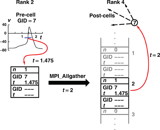
Figure 1. How the Allgather method communicates a spike event by a cell on rank 2 to target cells on rank 4. The illustration uses a maximum integration interval of 1 ms, a buffer size that can hold information about two spikes, and assumes no overflow on any rank during the computation interval between 1 and 2 ms. During the computation interval, a cell on rank 2 fires and its firing time and identifying number are placed in the send buffer and the buffer spike count is incremented. At the end of the computation interval, 2 ms in the illustration, MPI_Allgather sends the contents of its buffer to all other machines (only the receive buffer for rank 4 is shown). Note that the total receive buffer is the size of a send buffer times the number of processes ordered by rank. When MPI_Allgather returns (t is still 2 ms), each process checks all the spikes in its receive buffer by doing a hash table lookup using the cell identifier as key. If a source object for one or more Network Connection objects is returned, the source object with its minimum target destination time is placed on the queue. The computation interval from 2 to 3 then begins.

For performance testing, MPI_Barrier was placed before the MPI_Allgather to allow the distinction between synchronization waiting due to variation in the time to compute the integration interval, and the actual spike exchange time. A high-resolution clock counter (increments approximately every nanosecond) was saved on entry to Allgather, after MPI_Barrier, MPI_Allgather, and exit from Allgather.

Multisend

The DCMF Multisend family of non-blocking collectives provides a DCMF_Multicast function that allows a source processor to send the same message to a list of target processors. The message transfer over the network is managed on the BG/P by a DMA engine so that the compute cores are not involved in packet management and therefore, are fully available for computation at the same time that communication is taking place. In fact, MPI_Isend is implemented as a DCMF_Multicast with merely a list of one target.

To provide the possibility of greater overlap between computation and spike exchange when a spike occurs close to the end of an integration interval, the NEURON simulator implementation of the Multisend method for spike exchange provides the option of dividing the minimum delay integration interval (during which spikes are generated by neurons but are not needed on other processors until a subsequent interval) into two equal sub-intervals, call them A and B. Then a spike generated in sub-interval A, which immediately initiates a DCMF_Multicast that proceeds in the background, does not have to be delivered until after sub-interval B completes and vice versa. This allows significant time for the DCMF_Multicast to complete, in the sense that spikes have arrived at the target processors, during normal computation time. As long as a multisend completes in less than the sub-interval computation time, the time taken to actually transmit spikes should not contribute to the run-time. Each cell contains a list of target processors that need the spike generated by that cell and this list is determined during setup time based on the distribution of cells on the processors. When a spike is generated and DCMF_Multicast initiated, the count of sent spikes in the sub-interval is incremented by the size of the list. The DCMF_Multicast has enough space (16 bytes) in its header packet to contain the integer source cell identifier, the current A or B sub-interval, and double precision spiketime. Therefore, spike compression is obviated and no packet assembly is needed on the target processor.

Spike messages arriving at the target processor indirectly cause a callback to an incoming spike function registered by NEURON. This function increments the count of received spikes for the appropriate sub-interval and the spike information is appended to the sub-interval's incoming spike buffer. At least every time step, the buffered incoming spikes are moved into the priority queue by using a hash table look-up of the source object for all the network connection objects that have targets on that processor and enqueueing the source object at a time corresponding to the spike time plus the minimum connection delay to those targets. Just before starting a sub-interval's computation phase, the conservation of sent and received spikes is checked with MPI_Allreduce and, if total number sent is not equal to the total number received, a loop is entered which handles incoming spikes and moves them into the priority queue until conservation is satisfied according to MPI_Allreduce. When conservation of spikes is satisfied computation continues.

A minor DCMF detail alluded to above is that a spike message arriving at the target processor does not directly interrupt computation to call the incoming spike function callback registered by NEURON. Instead, the callbacks are made when the DCMF_Messager_advance function is called and we do this at least every time step and conservation iteration.

Figure 2 illustrates, for the generic Multisend method, the flow of spike information from the cell where the spike was initiated to the destination targets on another process.

FIGURE 2

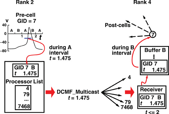
Figure 2. How the Multisend method communicates a spike event by cell 7 on rank 2, to target cells on rank 4. The illustration uses a maximum integration interval of 1 ms each of which is divided into two sub-intervals, A and B. During the A sub-interval, a cell on rank 2 fires, immediately starts the multisend transfer, here DCMF_Multicast, which initiates the non-blocking sends of the spike to all the ranks which have one or more cells, which are targets and increments the send count for the next interval by the number of destination ranks. The DCMF_Multicast returns immediately and computation on rank 2 continues, overlapping the transfer of messages from rank 2 to all the destination ranks indicated in the processor list for the source cell. The message is the same for all the destination ranks and consists of the spike initiation time, the source cell global identifier, and the next sub-interval at the end of which the spike must be received by all the ranks. When a message is received, e.g., by rank 4 in the illustration, the spike information is appended to the appropriate buffer for the sub-interval of the message, in this case Buffer B, and the receive count for that sub-interval is incremented by 1. At the end of each sub-interval, a loop of MPI_Allreduce operations is performed, so every rank knows the total number of messages sent and received, until those totals are equal. Occasionally during the sub-interval computation and certainly by the end of the MPI_Allreduce loop, the spike information in the sub-interval buffer is transferred to the event queue by doing a hash table lookup using the source cell identifier as key. The source object for the one or more Network Connection objects certainly exists in the table and that source object with its minimum target destination time is placed on the queue. Note that due to the MPI_Allreduce loop, synchronization of all ranks takes place at the end of each sub-interval.

For performance testing, MPI_Barrier was placed before the MPI_Allreduce to distinguish between synchronization waiting due to variation in the time to compute the integration interval and the underlying latency of the MPI_Allreduce. The high-resolution clock counter mentioned earlier was saved before the MPI_Barrier and before and after the conservation loop. From the beginning of an integration interval to the beginning of the following integration interval, total clock counter intervals were also saved for source object lookup using the hash table, for enqueueing the source object, and for the time needed to initiate a Multisend.

MPI point-to-point

In the above algorithm, the call to DCMF_Multicast can be replaced by a loop over destination target processors of individual calls to non-blocking MPI_Isend. MPI_Isend on BG/P has startup overheads such as resource allocation, C++ object construction, translation of virtual addresses to physical addresses, and construction of the DMA descriptor. The DCMF_Multicast call has lower overheads as it is a single call with a single startup to allocate all resources, translate the address once, and construct the descriptor once as well and then injecting multiple descriptors by just changing the destination field in the descriptor. With MPI_Isend, the polling of DCMF_Messager_advance within integration intervals and within the conservation loop is also replaced by a loop which checks MPI_Iprobe to determine if a message has arrived. If so, the spiketime, Global Neuron Identifier (GID), and sub-interval identifier is extracted from a MPI_Recv received message and the spiketime and GID appended to the proper sub-interval buffer.

Multisend method variations

As will be seen, there can be high variance in computation and spike exchange time for integration intervals within a simulation and this leads to excessive load imbalance. This led us to investigate several variations of the two-sub-interval Multisend and MPI point-to-point methods.

An obvious variation is the use of a single sub-interval. In this case, any spike generated in the last time step of the full “minimum network connection delay integration interval” must make its way to the target machines during the conservation loop.

Another variation is the use of a two-phase strategy for sending spikes to target processors. Instead of sending an output spike to all N_t target processors, it is sent to only a subset of size target processors. When a spike is received by one of these target processors, that target processor initiates a Multisend to a size subset of the remaining target processors. In particular, setup time determination of the spike distribution patterns is accomplished in several steps. First, the list of N_t target processors of an output cell (the phase-one sender) is partitioned into subsets of size approximately equal to the integer square root of N_t. Second, one of the target processors in each subset is randomly selected (specifies the phase-one target processor list) and the subset list for each phase-one target processor, is sent to that target where it is saved as the phase-two target list of the source object (phase-two sender) associated with the specified global cell identifier. Note that there is no attempt to use torus distance between machines to select subsets or the phase-two sender. Both phase-one and phase-two sending and receiving is identical to that described above for the Multisend method but note that conservation will not be satisfied until the phase-two receives have completed. If there are two sub-intervals, we have observed very much better load balance when a phase-two send is not allowed in the sub-interval of the phase-one send but is forced to take place in the following sub-interval (Incoming spikes are buffered and after each DCMF_Messager_advance, only the buffered spikes required to be received by the end of the current integration sub-interval are enqueued). In our first implementation of the two-phase method, we imagined that it would be helpful to allow phase-two spikes more time to make their way to the target processors and therefore, also tried initiating phase-two sends as needed for spikes in both sub-interval buffers. This resulted in a curious and very large load imbalance where phase-two spike exchange initiation time would interact with the sub-interval computation time so that, independently of which interval initiated a phase-one send, significantly more phase-two send initiation would occur in one interval rather than the other. Thus, the time used by adjacent sub-intervals oscillated by a large amount and some processors would have consistently longer A sub-interval durations and the others would have consistently longer B sub-interval durations. This problem did not occur when phase-one and phase-two sends were initiated in different sub-intervals.

The final variation is the use of the Record-Replay feature of DCMF_Multicast. For normal DCMF_Multicast, every time a cell fires, its target list gets copied into one of a few descriptors whose head and tail pointers are then given to the DMA network communication engine. For the Record-Replay method a separate descriptor is maintained for each cell. Only when the cell first generates a spike does the target list get copied to the unique descriptor for the cell. Subsequent firing of the cell only involves giving the head and tail pointers of the proper descriptor to the DMA engine. Thus, initiation overhead is extremely low.

Test model

In order to focus on spike exchange performance we use the artificial spiking cell network (Kumar et al., 2010) designed to minimize computation time.

Each artificial spiking cell fires intrinsically with a uniform random interval between 20 and 40 ms, i.e., average 30 Hz firing frequency. Computation time of the artificial spiking cell is proportional to the number of input spikes to the cell and number of generated spikes by the cell and consists, for each input and generated spike, mostly of evaluation of an exponential and logarithm function. The exponential evaluation determines the value of the cell state variable, m, given the state value, m₀ when previously calculated at time, t₀.

where, the steady state is chosen so that the state variable moves from its initial value, 0, to its firing trigger value, 1 in the randomly chosen interval, t_i.

A self-notification event is added to the event queue with a delivery time of t_i. A spike input modifies the interval to the next output spike of the cell by discontinuously changing the m state variable,

where, w is the weight of the specific source to target network connection that delivers the spike to the target cell. If the cell's self-notification event is moved to the current time. Otherwise, evaluation of a logarithm function updates the (future) firing time of the cell's output spike,

by moving the self-notification event to t_f. When the self-notification event is delivered, the cell generates an output spike event, m is set to 0, and a new self-notification event is added to the event queue with a new random delivery time, t_i. Note that excitatory events (positive weight) decrease the interval between output spikes and inhibitory events (negative weight) increase the interval between output spikes.

Networks consisted of N = 256 K–32 M cells (K = 1024, M = K², and k = 1000). Each cell is randomly connected to approximately C = 1 k or 10 k other cells (the number of connections is drawn from a uniform random distribution ranging from where is typically 100). The connection delay is 1 ms. All connection weights are set to 0 in order to maintain each cell's random firing behavior and eliminate any connection dependent response behavior that might arise due to the size of the network or the specific random connectivity. The 0 weights do not affect, or at least do not increase, cell computation time. Since each cell is associated with a distinct statistically independent but reproducible random generator, the specific random network topology and specific random firing of each cell is independent of the number of processors or distribution of cells among the processors.

Simulation runs are for 200 ms. That is 200 integration intervals for the Allgather spike exchange method and 200 integration intervals or 400 A-B integration sub-intervals depending on whether the use of one or two sub-intervals was chosen for the Multisend methods. Simulations were run on 8–128 K cores of the BG/P. As 512 MB memory is available for each core and NEURON has heavy weight network connections, not all combinations of N, C, and number of cores could be used.

Results

Figure 3 illustrates the spiking behavior of the model (with 256 cells) as a raster plot. Notice that because a cell certainly fires from 20 to 30 ms after its previous firing, there is an initial interval of 20 ms with no spikes followed by a subsequent 20 ms in which all cells fire. The average frequency of the whole network oscillates for a few intervals before settling to a constant rate.

FIGURE 3

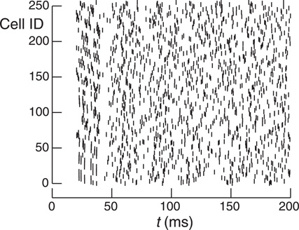
Figure 3. Raster plot shows the spike time as short vertical lines for each of 256 cells (Cell ID integers range from 0 to 255) for a 200 ms simulation. Cells spike randomly with a uniform distribution from 20 to 40 ms.

Figure 4 shows how run-time varies with number of processors for the Allgather, two-phase two-sub-interval MPI_Isend, two-phase two-sub-interval DCMF_Multicast, and one-phase one-sub-interval Record-Replay methods. For each Multisend method, the choice of one or two sub-intervals and one or two-phases was determined by which gave the best performance. In general, use of the DCMF_Multicast methods result in a three-fold faster run-time than the MPI_Isend method. This can be attributed to the relatively high overhead for short messages since incoming sends need to be matched with posted receives as well as the extra overhead of a large number of independent send and receive calls. As expected, the Allgather method compares favorably with the point-to-point methods when most machines need most spikes. Thus, with 10 k connections per cell and 1 M cells, the Allgather method is still best with this model at 32 K processors. With this size model and number of processors there is a cell on rank 0 that needs to send spikes to 8791 other processors and there is a cell that needs to send spikes to 8999 other processors. For 1 k connections per cell both strong and weak scaling is close to ideal over the range of processors explored for the multisend methods.

FIGURE 4

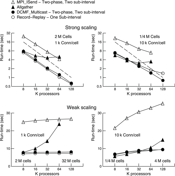
Figure 4. Strong and weak scaling performance for 1 k connections per cell (left) and 10 k connections per cell (right). For strong scaling 2 M and 1/4 M cells were simulated, respectively. For weak scaling, the number of cells was proportional to the number of processors used and ranged from 2 M to 32 M cells and 1/4 M to 4 M cells, respectively. The number of processors used ranged from 8 K to 128 K. Filled triangles show the performance (real time seconds for a 200 ms simulation) for the Allgather method (one sub-interval). Open triangles are for the MPI_Isend two sub-interval, two-phase method. Filled circles are for the DCMF_Multicast two sub-interval, two-phase method. Open circles are for the Record-Replay DCMF_Multicast method with one sub-interval and one-phase. Note the log-log scale for strong scaling with a dashed line indicating the ideal scaling slope of −1.

Tables 1 and 2 present the run-time values plotted in Figure 4 along with the time that can be attributed to computation by processor rank 0. Computation time is measured as the time used from the beginning to the end of integration intervals. For Multisend methods, spike communication overlaps with integration and all spike handling within the interval is charged to computation time. That is, when an incoming spike arrives during an integration interval, the computation time consists of the time to: 1) determine the correct source object from the arriving integer global identifier, 2) enter it onto the priority queue for delivery at the spike generation time plus minimum target cell connection delay, 3) deliver the spike to the targets when the delivery time matches the simulation time, 4) compute the change in state of the artificial cell (evaluation of an exponential function), and 5) move the next firing time of the cell to a new value (evaluation of a logarithm). Cell state dependent additions to the computation time include the issuing of a new spike event if the state is greater than 1. That is, the time required for the initiation of non-blocking interprocessor communication which, for the MPI_Isend method, involves iteration over the target processor list of the spiking cell. For the Allgather method, computation time does not include the finding of the correct source object or enqueuing that object; issuing a spike event merely adds the spike information to a send buffer. The difference between run-time and the computation time of rank 0 is the wait time for global processor synchronization (measured by the time it takes for an MPI_Barrier call to return), along with either the Allgather exchange time or, for Multisend methods, the time it takes to verify that the number of spikes sent is equal to the number of spikes received. Note that the handling of spikes arriving during the conservation step or Allgather (finding and enqueuing the source object) is charged to exchange time instead of computation time.

TABLE 1

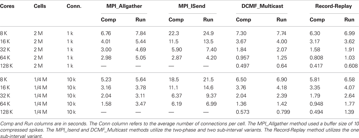
Table 1. Strong scaling performance of NEURON (seconds) on BG/P in Virtual Node mode for simulation runs lasting 200 ms.

TABLE 2

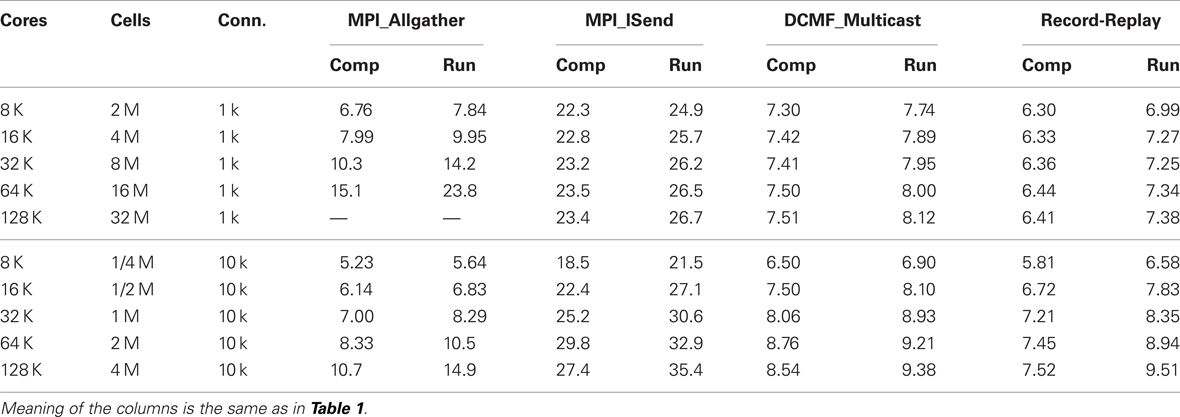
Table 2. Weak scaling performance of NEURON (seconds) on BG/P in Virtual Node mode.

To understand the difference between run-time and computation time it is useful to plot both for each integration interval (or sub-interval). We first consider the Allgather method.

Figure 5 shows the number of processor clock ticks on rank 0 for each integration interval during a 200 ms simulation (One million clock ticks is 1.17647 ms). Three different compressed spike buffer sizes for the MPI_Allgather communication phase on 16 K processors were used and are indicated in each panel. The overall shape of the three simulations is governed by the 20–40 ms uniform random interval for cell spiking. That is, no spikes for the first 20 ms, followed by all cells spiking in the next 20 ms. Just after 40 ms, there is very little spiking since all cells are in their interspike interval and so there are no input spikes to the cells. After a few 20 ms cycles the whole network spiking frequency becomes constant. A single spike requires two bytes of information: one byte to specify the local identifier (there are 256 or fewer cells per processor) and one byte to specify the dt step within the interval. For these simulations, dt = 25 μs and the maximum integration interval is 1 ms, so there are 40 dt steps per interval. Of course, the computation time is independent of the MPI_Allgather send buffer size and even the noise details are identical in the three panels. There is very little noise at the adjacent interval level in the computation time. Also, notice that there is a similar degree of noise for total time per interval when the 40 spike send buffer is large enough so that an MPI_Allgatherv communication phase to send overflow spikes is never needed. Finally, notice that for the 40 spike send buffer, the difference between total time per interval and computation time per interval is apparently constant for the duration of the simulation. This is consistent with the observation that the variation in number of input spikes handled by different processors is fairly small. During the initial 20 ms, it is clear that MPI_Allgather time doubles as the send buffer size doubles. On the other hand, the smaller the send buffer, the more often it is necessary to use MPI_Allgatherv to send overflow spikes. Regardless, load balance among the processors is excellent with the Allgather method.

FIGURE 5

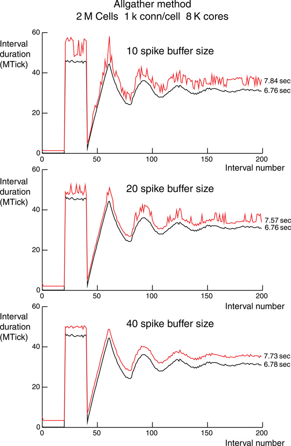
Figure 5. Per interval performance for the Allgather method for three different compressed spike buffer sizes which allow 10, 20, or 40 spikes to be sent by MPI_Allgather before requiring the use of an MPI_Allgatherv for sending the remaining overflow spikes. The spike buffer sizes are indicated in the panels. Each simulation is for 2 M cells with 1 k ±50 connections per cell on 8 K processors. Simulation time is 200 ms and each connection has a spike delay of 1 ms, i.e., 200 integration intervals. The ordinate is millions of processor clock ticks with 1 tick = 1.17647 ns. Black lines are computation time per interval and includes finding and enqueuing the Network Connection source object using the received spike information. Red lines are total time per interval. The difference is a measure of load imbalance and spike communication time. Noise in the red line mostly reflects the extra time taken by overflow spike communication using MPI_Allgatherv. Total computation and simulation time, sum of the times for each interval, is indicated just to the right of each line.

In contrast, load imbalance within the DCMF_Multicast method significantly increases the run-time as can be seen in Figure 6 for 4 M cells with 1 k connections per cell on 16 K processors and Figure 7 for 2 M cells with 10 k connections per cell on 64 K processors. The thin black line in each figure panel is the rank 0 computation time. The thick black line is the average computation time for all processors. The dashed black line is the maximum computation time for all processors and in most of the panels is not visible due to its being hidden by the red total interval time. The dashed line is visible only in the two-phase, one-sub-interval panels. This processor computation load imbalance is largest for the one-phase, two-sub-interval simulations where there is the largest variation in spikes generated per interval. That is, when a spike is generated, significant time is needed to initialize a multisend. The number of spikes per interval generated on the 256 cells of rank 0 over the last 50 ms of simulation ranges from 1 to 8 spikes per interval with a consequent sending of 919–7799 spikes per interval to other processors. This is in contrast to receiving 3954–4400 spikes per interval, i.e., much smaller variance. Note that a single cell on rank 0 sends spikes to at most 1049 processors and there is a cell on some rank that sends spikes to 1129 distinct processors. This may seem puzzling at first since no cell can receive spikes from more than 1050 source cells but there is no constraint on how many targets a single source cell can have. In this simulation, communication entirely overlapped with computation and there was no interval in which the conservation test using MPI_Allreduce did not succeed on the first iteration. An obvious strategy to reduce the spike output variance is to eliminate the two sub-intervals in favor of a single interval, i.e., all spikes generated in an interval must be received before the beginning of the next interval. In this case the statistics for the last 50 ms (50 intervals) of simulation are 3–16 spikes per interval generated, 2798–15,619 spikes per interval sent, and 8033–8719 spike per interval received. Surprisingly, conservation again succeeded always on the first iteration. The variance in number of cells that fire cannot be reduced. However, the two-phase spike propagation method can be used to more evenly distribute the number of spikes sent from each processor. In this case, since a generated spike is sent to about 30 other target processors and then each receiving processor passes it along to about 30 other target processors, there is a significant number of conservation iterations needed for all the spikes in an interval to arrive before the beginning of the next interval. That is indicated by the difference between the dashed line and the red line in the two-phase, one-sub-interval panels. In fact, two iterations are needed for a total of three MPI_Allreduce calls per interval. Since the Multisend time variation is now minimal with the two-phase method, the two-sub-interval method can be used so that conservation succeeds on the first MPI_Allreduce and that combination gives minimal run-time.

FIGURE 6

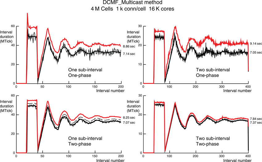
Figure 6. Comparison of per interval performance of the DCMF_Multicast method using one (top) and two (bottom) phase spike exchange, and one (left) and two (right) sub-intervals for each maximum integration interval. For one sub-interval the number of intervals for a 200 ms simulation is 200 and for two sub-intervals the number is 400. Note that the ordinate scale is half for the two sub-interval simulations and reflects the roughly half amount of time required needed by each (sub)interval. Each simulation is for 4 M cells with 1 k ±50 connections per cell on 16 K processors. The red lines are the total time per interval. The thin black lines are the computation time per interval for the rank 0 processor. The thick black lines are the average computation time for all ranks. The dashed black lines, visible only in the one interval, two-phase simulation is the maximum computation time for all ranks. Dashed black lines in the other three simulations are overlaid by the red lines. Black lines include all spike handling time during an interval. The difference between red and black lines is the MPI_Barrier time for synchronization of all ranks along with the conservation loop involving MPI_Allreduce and residual spike handling. Total computation and simulation time for rank 0 is indicated just to the right of each red and thin black line.

FIGURE 7

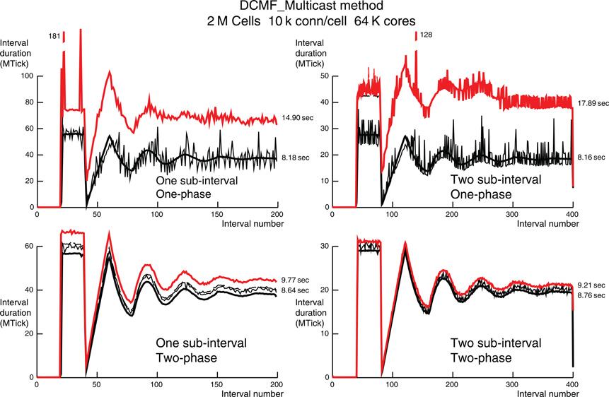
Figure 7. Like Figure 6, but for 10 k ±50 connections per cell, 2 M cells and 64 K processors. The two large intervals in the one-phase simulation that do not fit on the graph are labeled with their interval times in MTicks.

The forgoing discussion of Figure 6 also applies to Figure 7 with 32 cells per processor, 64 K processors, and at most 10,050 source connections per target cell. However, in Figure 7 the corresponding statistics are: The cell on rank 0 that has the most target processors sends spikes to 9476 processors; the greatest fanout for any cell is 9787 processors; In the last 100 intervals of the two-sub-interval one-phase simulation, 0–4 cells fire per interval on rank 0, 0–37,175 spikes are sent, and 4703–5271 spikes are received. In the last 50 intervals of the one-sub-interval one-phase simulation, 0–5 cells fire per interval on rank 0, 0–46,489 spikes are sent, and 9577–10,386 spikes are received. In both simulations, no conservation iterations are needed. Just as in the corresponding simulation for 1 k connections per cell, the two-phase, one-sub-interval method requires two conservation iterations per interval. Again, the two-phase, two-sub-interval method is best with its maximization of load balance and minimization of conservation iterations. We have no definitive explanation for the occasional very long computation times for a single interval on some processor (the dashed black line is hidden by the red line on the plots). However, those outliers do not significantly affect the total run-time.

Load-imbalance due to the variance of cell firing can also be reduced by avoiding DCMF_Multicast initiation overhead through the use of the Record-Replay feature for DCMF_Multicast. When a cell fires for the first time, the Record operation copies the list of target ranks to a message descriptor and stores each message descriptor in a separate buffer. Subsequent firing of that cell uses the Replay operation to merely set the head and tail pointers in the DMA descriptor to that buffer, avoiding the overhead of copying the list of target ranks.

Figure 8 uses the Record-Replay feature to show time per interval results for one- and two-sub-interval simulations corresponding to the one-phase simulations of Figures 6 and 7. Notice that for the first 40 ms, noise is very similar to the normal DCMF_Multicast method since all cells fire for the first time and so are using the Record operation which copies the target rank list. For subsequent firing, the DCMF_Multicast Replay initialization is negligible and load balance of all processors within each interval is excellent, i.e., compare the average computation time per interval (thick black line) to the maximum computation time per interval for all ranks (thin dashed black line). For the one-sub-interval simulations, the conservation iterations are 0–14 and 2–231 for 1 k and 10 k connections per cell, respectively. In contrast, the conservation iterations for the two-sub-interval simulations are 0–554 and 0–1025, respectively. In tests of the Record-Replay method we have found it important to frequently poll for incoming messages with calls to DCMF_Messager_advance and presently do that every time step, every 50th synaptic event, and each conservation iteration. It is also done in a loop while a message descriptor is in use but, since there is a separate descriptor for each cell with this method, that is irrelevant. The excessive number of conservation iterations for the two-sub-interval simulations—which should be fewer than for the one-sub-interval simulations given, the guarantee of an entire sub-interval of computation between initiation of a message and its receive completion, seems to suggest a potentially fixable problem either in our use of Record-Replay or its internal implementation. Nevertheless, the one-sub-interval Record-Replay method has slightly better performance than the two-sub-interval two-phase DCMF_Multicast method for this model. Also, Record-Replay would be slightly more advantageous when the Record operation is amortized over a longer simulation time.

FIGURE 8

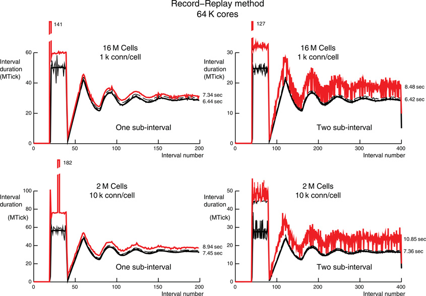
Figure 8. Record-Replay per interval performance for 1 k (top) and 10 k (bottom) connections per cell on 64 K processors (16 M and 2 M cells on top and bottom, respectively). The style for the top and bottom are the same as the one-phase simulations (top) of Figures 6 and 7, respectively. The three large intervals that do not fit on the graph are labeled with their interval times in MTicks.

It is clear from the simulations presented so far that optimum performance requires that the number of synaptic input events within an integration interval be similar for all ranks. In practice, load balance may be impossible to achieve when small subsets of cells dynamically undergo increased activity and their target cells consist of a small fraction of the total number of cells. In order to examine the effect on load balance of increased burst activity within subnets, the network was divided into N_g groups of N/N_g cells with contiguous GIDs within each group successively exhibiting increased firing rate. Figure 9 illustrates this with a raster plot for a network with N_g = 8, N = 256 cells, and therefore, a group size of 32 cells. Each group successively has a five fold increase in firing rate over an interval of 50 ms.

FIGURE 9

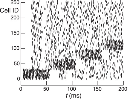
Figure 9. Raster plot of 256 cells with 32 contiguous cell group size. Cells normally spike randomly with the uniform distribution from 20 to 40 ms. However, each group successively increases its spiking rate by a factor of 5 for 50 ms. Note that the seeming group dead time when the group returns to its normal firing rate where each cell has minimum interval of 20 ms since its last firing. cf. Figure 3.

Table 3 shows the computation and run-time for N_g = 8 simulations of 4 M cells with 1 k connections per cell on 16 K processors with and without five-fold increase in burst firing rate within successive groups. The table allows comparison between three distributions of GIDs on the processors and two connection topologies. The “random” connection topology is that used in the previous figures. The “adjacent” connection topology means that each target cell is connected to its 1000 nearest neighbor cells (in terms of GID values). The “round robin” distribution is that used in the previous figures. The “random shuffle” distribution means that cells are randomly distributed among the ranks with each rank having the same number of cells. The “consecutive” distribution means that cells with GID 0–255 are on rank 0, cells with GID 256–511 are on rank 1, etc. Note that with the consecutive distribution and adjacent connections, cell firing needs to be communicated to only five other ranks. Furthermore, since all delays are the same, then, when the source object on the target machine reaches the head of the queue, delivery of the event to the 256 target cells on a host takes place with no need for further delay on the queue. This is the reason for the much smaller computation and run-times in the absence of bursting. Here, the number of arriving events per interval for each rank is just five times greater than the average number of output events per rank and so the time for finding the source object and managing the source events on the priority queue has become negligible compared to the computation time involved in the over 200-fold greater number of synaptic events. On the other hand, bursting ruins the load balance since successive groups of ∼2 K ranks are receiving five times the number of spikes than each of the remaining ranks in the 16 K set. For this simulation, the consequence is that the run-time performance is similar to the other GID distribution methods.

TABLE 3

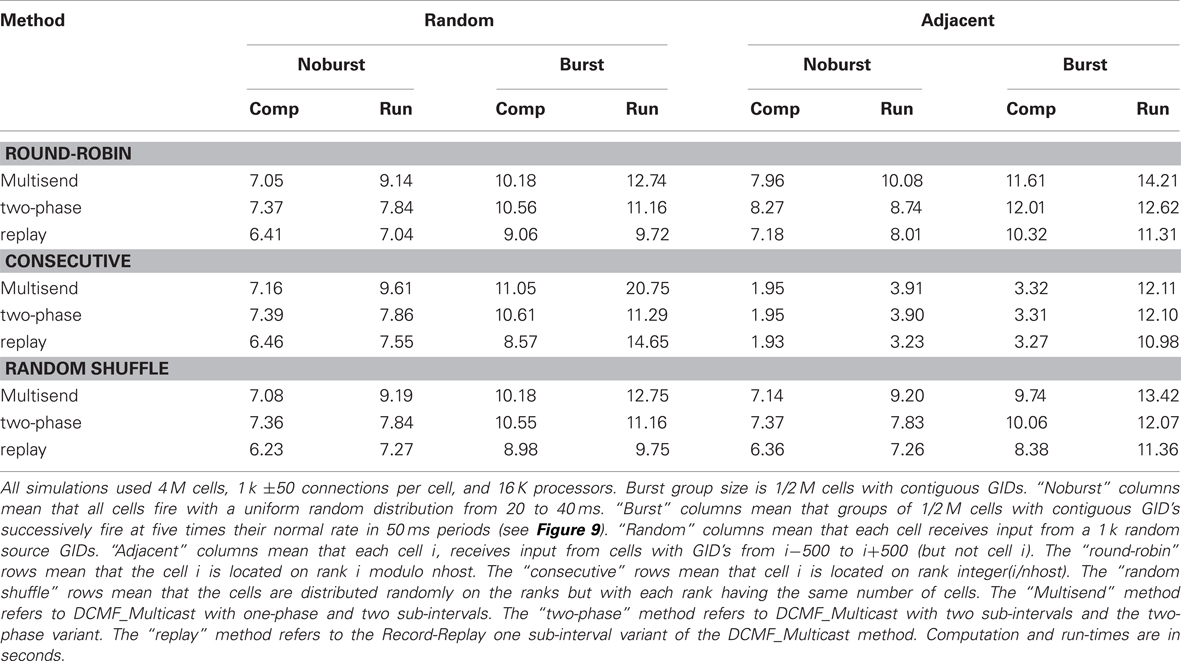
Table 3. Uniform and burst firing performance for random and adjacent connectivity, three cell distribution algorithms, and three spike exchange methods.

Discussion

All the Multisend methods we tested exhibit complete overlap of communication within the computation interval except for Record-Replay with 10 k connections per cell. In particular, the MPI_Isend implementation of multisend also exhibits complete overlap. The difference between computation time and total time is almost entirely due to load imbalance with respect to the number of incoming messages per processor within integration intervals. Load imbalance due to high variance of cell firing within an interval is greatly alleviated, either through the use of Record-Replay operations of DCMF_Multicast, or with a two-phase message propagation strategy which uses processors to send messages to the N_t target processors of the spiking cell.

The fact that overlap is complete, even for one-sub-interval Multisend methods with the largest number of processors used, seems a particularly impressive property of the BG/P communication system. That is, a message sent during a single time step to 1000 processors distributed randomly over the machine topology, reaches all its destinations before the beginning of the next time step. On even the largest partition sizes used, there is no reason yet to consider more sophisticated distribution schemes that would attempt to minimize the total message propagation distance.

Although MPI_Allgather is a blocking collective, overlap between computation and spike exchange may be possible through the use of threads. With two sub-intervals for each minimum network connection delay interval, a high priority spike exchange thread would initiate MPI_Allgather at the end of one sub-interval. While the spike exchange thread was waiting for completion of the MPI_Allgather, a low priority computation thread could continue until the end of the other sub-interval. During computation, completion of the MPI_Allgather would occasionally initiate an MPI_Allgatherv asynchronously in the spike exchange thread within that other sub-interval. Finally, the computation thread would also wait for completion of the MPI_Allgather(v) at which point, spike exchange would be initiated for the spikes generated during the other sub-interval. Unfortunately, this strategy cannot be tested on the BG/P since only one thread per core is allowed. For machines without the single thread per core limitation, it would be an experimental question whether, during MPI_Allgather processing/communication, the CPU is actually available for computation and whether the savings would be greater than the cost of thread switching. In any case, the rate of increase in MPI_Allgather time as the number of processors increases, means that MPI_Allgather time will eventually dominate computation time.

An alternative to repeated use of MPI_Allreduce within a conservation loop is to explicitly receive the count of spikes that should arrive at each individual target processor by using MPI_Reduce_scatter (Ananthanarayanan and Modha, 2007) and then calling MPI_Recv that many times to receive all the messages destined for that target processor (or, for the DCMF_Multicast method, entering a DCMF_Messager_advance loop until that many messages arrive). Since conservation loop timing results show that the time charged to the MPI_Allreduce portion, and indeed, usually the entire conservation loop itself, is negligible on up to 128 K processors, we have not compared MPI_Reduce_scatter to MPI_Allreduce performance. Note that the use of MPI_Reduce_scatter would vitiate some of the load balance benefits we saw with the Record-Replay method. That is, a spike generated on the source processor would require an iteration over the processor target list of the source cell in order to increment the count of sent spikes to those processors and thus increase dynamic load imbalance.

The excessive number of conservation iterations for Record-Replay with 10 k connections per cell is most likely attributable to the fact that the current implementation of Record-Replay only permits messages for one cell's spikes to be sent out at a time. A call to DCMF_Messager_advance after the current cell's spikes have been sent out is needed to trigger the data transfer for the next cell. In the future, we plan to explore techniques that can accommodate cell spike data transfer in the same way as the standard DCMF_Multicast implementation, and that should further improve the performance of the Record-Replay technique.

Our first weak scaling run attempted on 128 K processors (32 K nodes) did not succeed because 184 of the processes raised a “can't open File” error on the Hoc file specified at launch. Since the expected boot time of that size partition is 12 minutes, a minimal test run which exits immediately uses at least 26,000 CPU hours. In fact, the job waited until it timed out after an hour thus wasting almost 140 k CPU hours. To scale-up to larger processor numbers it was necessary to avoid the huge numbers of replicated reads by having rank 0 read the Hoc file and broadcast it to all ranks, which then execute the buffer contents.

There exists a DCMF_Multicast operation which can send different data to its list of targets. This would allow very significant reduction in the lookup time on the destination processor for lookup of the source object associated with the source GID. That is, instead of a hash table lookup, the index into a list of source objects on the destination processor would be sufficient. Prior to a simulation run, the proper destination list indices would be stored along with each cell's list of destination processors. This optimization is used, for example, by MUSIC (Djurfeldt et al., 2010) in its spike exchange algorithm. However, this optimization may be vitiated by the loss of an existing optimization that we use where the user portion of the message is empty and the (i, t_s) information is encoded in the header so only a single packet arrives—thus, software overhead of waiting for and assembling the packets is avoided.

The Table 1 strong scaling results on 8–32 K processors for the 1/4 M cell, 10 k connections per cell simulations are from two to three times faster than the results shown in Table 2 of Kumar et al. (2010). The largest part of the improvement for DCMF_Multicast comes from the use of two-phase method, and for Record-Replay, the use of DCMF_Messager_advance for each time step.

The size of networks used in this study has been limited due to the memory needed by NEURON's network connection objects. These objects use reciprocal pointers to their source and target objects as well as to wrapper objects at the interpreter level. Those pointers are required only for purposes of maintaining consistency when the user modifies a cell or eliminates a connection and the wrapper objects themselves are only needed transiently during setup time. NEURON's use of double precision delay and weights for each connection is another place where the memory needed by connections can be reduced. There exist artificial spiking cell simulators such as NEST whose network connection memory footprint has been minimized (Kunkel et al., 2009). In those simulators, networks with many more cells on the same number of processors could be simulated and it would be interesting to see if the Multisend method's complete overlap we see between computation and spike communication would be maintained in those environments. That would be expected on the grounds of the almost linear relation between computation time and number of cells. And with more cells, spike input balance is even less of a problem.

Record-Replay and the two-phase Multisend method solve the load balance problems due to high processor variance in cell firing within an interval. However, it is clear that load balance in terms of spike input to the sets of cells on processors will become a much more vexing issue with more realistic neural networks where populations of cells having a large dynamic spiking range have multiple projections to other populations. That is, input activity is generally also correlated in time and space. For example, Ananthanarayanan et al. (2009) report that for their extremely large-scale simulations (0.9·10⁹ cells, 0.9·10¹³ synapses, 144 K cores, and using MPI_Isend) 60–90% of the time was consumed in an MPI_Barrier due to the variability in firing rate. Our results supply strong evidence that one should neglect efforts to minimize spike exchange time through any kind of matching of populations to subsets of nearby processors in favor of promoting load balance by distributing these populations over as wide a number of processors as possible. Thus, networks in which connections are to nearest neighbor cells and all cells fire uniformly, give only a two-fold performance improvement when this connection topology is exploited through the use of placing neighbor cell sets on the minimal set of adjacent processors. But this performance improvement disappears as soon as cell groups begin to burst. Thus, in the same way that the very simple Allgather method provides a baseline for comparison with alternative spike exchange methods, the simple random distribution of cells evenly on all processors provides a performance baseline for comparison with more sophisticated distribution algorithms.

Conflict of Interest Statement

The authors declare that the research was conducted in the absence of any commercial or financial relationships that can be construed as a potential conflict of interest.

Acknowledgments

Research supported by NINDS grant NS11613 and The Blue Brain Project. Philip Heidelberger, Dong Chen, and Gabor Dozsa of IBM, Yorktown, gave us invaluable advice on the use of DCMF_Multicast. The research presented in this paper used resources of the Argonne Leadership Computing Facility at Argonne National Laboratory, which is supported by the Office of Science of the US Department of Energy under contract DE-AC02-06CH11357.

References

Ananthanarayanan, R., Esser, S. K., Simon, H. D., and Modha, D. S. (2009). “The cat is out of the bag: cortical simulations with 10⁹ neurons and 10¹³ synapses”, in Supercomputing 09: Proceedings of the ACM/IEEE SC2009 Conference on High Performance Networking and Computing Portland, OR.

CrossRef Full Text

Ananthanarayanan, R., and Modha, D. S. (2007). “Anatomy of a cortical simulator”, in Supercomputing 07: Proceedings of the ACM/IEEE SC2007 Conference on High Performance Networking and Computing, Reno, NV.

CrossRef Full Text

Djurfeldt, M., Hjorth, J., Eppler, J. M., Dudani, N., Helias, M., Potjans, T. C., Bhalla, U. S., Diesmann, M., Kotaleski, J. H., and Ekeberg, O. (2010). Run-time interoperability between neuronal network simulators based on the MUSIC framework. Neuroinformatics 8, 43–60.

Pubmed Abstract | Pubmed Full Text | CrossRef Full Text

Djurfeldt, M., Johansson, C., Ekeberg, C., Rehn, M., Lundqvist, M., and Lansner, A. (2005). Massively parallel simulation of brain-scale neuronal network models. Technical Report TRITA-NA-P0513. Stockholm: School of Computer Science and Communication.

Eppler, J. M., Plesser, H. E., Morrison, A., Diesmann, M., and Gewaltig, M.-O. (2007). Multithreaded and distributed simulation of large biological neuronal networks. Proceedings of European PVM/MPI 2007, Springer LNCS 4757, 391–392.

CrossRef Full Text

Gewaltig, M.-O., and Diesmann, M. (2007). NEST (Neural Simulation Tool). Scholarpedia 2, 1430.

CrossRef Full Text

Hereld, M., Stevens, R. L., Teller, J., and van Drongelen, W. (2005). Large neural simulations on large parallel computers. IJBEM 7, 44–46.

Hines, M. L., and Carnevale, N. T. (1997). The NEURON simulation environment. Neural Comput. 9, 1179–1209.

Pubmed Abstract | Pubmed Full Text | CrossRef Full Text

Kumar, S., Heidelberger, P., Chen, D., and Hines, M. (2010). “Optimization of applications with non-blocking neighborhood collectives via multisends on the Blue Gene/P supercomputer”, in 24th IEEE International Symposium on Parallel and Distributed Processing.

CrossRef Full Text

Kumar, S., et al. (2008). “The deep computing messaging framework: generalized scalable message passing on the Blue Gene/P Supercomputer”, in The 22nd ACM International Conference on Supercomputing (ICS), Island of Kos, Greece.

CrossRef Full Text

Kunkel, S., Potjans, T. C., Morrison, A., and Diesmann, M. (2009). Simulating macroscale brain circuits with microscale resolution. Frontiers in Neuroinformatics. Conference Abstract: 2nd INCF Congress of Neuroinformatics.

CrossRef Full Text

Markram, H. (2006). The blue brain project. Nat. Rev. Neurosci. 7, 153–160.

Pubmed Abstract | Pubmed Full Text | CrossRef Full Text

Migliore, M., Cannia, C., Lytton, W. W., Markram, H., and Hines, M. L. (2006). Parallel network simulations with NEURON. J. Comput. Neurosci. 21, 119–129.

Pubmed Abstract | Pubmed Full Text

Tam, A., and Wang, C. (2000). “Efficient scheduling of complete exchange on clusters” in 13th International Conference on Parallel and Distributed Computing Systems (PDCS 2000), Las Vegas (August, 2000).

Wilson, E. C., Goodman, P. H., and Harris, F. C. (2001). “Implementation of a biologically realistic parallel neocortical-neural network simulator” in Proceedings of the Tenth SIAM Conference on Parallel Processing for Scientific Computing, March 12–14, 2001 Portsmouth, Virginia.