A statistical description of neural ensemble dynamics
- 1 Helen Wills Neuroscience Institute, University of California, Berkeley, CA, USA
- 2 Department of Electrical Engineering and Computer Sciences, University of California, Berkeley, CA, USA
- 3 Program in Cognitive Science, University of California, Berkeley, CA, USA
The growing use of multi-channel neural recording techniques in behaving animals has produced rich datasets that hold immense potential for advancing our understanding of how the brain mediates behavior. One limitation of these techniques is they do not provide important information about the underlying anatomical connections among the recorded neurons within an ensemble. Inferring these connections is often intractable because the set of possible interactions grows exponentially with ensemble size. This is a fundamental challenge one confronts when interpreting these data. Unfortunately, the combination of expert knowledge and ensemble data is often insufficient for selecting a unique model of these interactions. Our approach shifts away from modeling the network diagram of the ensemble toward analyzing changes in the dynamics of the ensemble as they relate to behavior. Our contribution consists of adapting techniques from signal processing and Bayesian statistics to track the dynamics of ensemble data on time-scales comparable with behavior. We employ a Bayesian estimator to weigh prior information against the available ensemble data, and use an adaptive quantization technique to aggregate poorly estimated regions of the ensemble data space. Importantly, our method is capable of detecting changes in both the magnitude and structure of correlations among neurons missed by firing rate metrics. We show that this method is scalable across a wide range of time-scales and ensemble sizes. Lastly, the performance of this method on both simulated and real ensemble data is used to demonstrate its utility.
Introduction
The growing use of multi-channel neural recording techniques in behaving animals has opened up new possibilities for understanding how the brain mediates behavior. These techniques are generating datasets that record the output of ever increasing numbers of neurons (Nicolelis et al., 2003; Suner et al., 2005; Nicolelis, 2008). Unfortunately, current recording techniques do not provide information about the underlying anatomical connections between the recorded neurons. Without these anatomical constraints, the set of possible network diagrams grows exponentially with increasing ensemble size. This limitation poses formidable challenges to the analysis and interpretation of these datasets (Palm et al., 1988; Averbeck et al., 2006). Several groups have focused upon the challenging inverse problem of inferring the connectivity among the individual neurons from ensemble data (Brown et al., 2001; Truccolo et al., 2005; Eldawlatly et al., 2009). However, the combination of expert knowledge and ensemble data is generally insufficient to select a unique model from the vast space of possible network diagrams. Thus, analysts are often faced with an intractable model selection problem (Sivia, 1996; Ghahramani, 1998).
A promising alternative comes from the field of statistical mechanics (Jaynes, 1957). This approach endeavors to estimate macro properties of a system, for example its entropy, from observations of its constituent parts. Recent applications of this approach in neuroscience have modeled the neural ensemble by maximizing its entropy subject to constraints imposed by estimated features of the neural ensemble. Importantly, these maximum entropy models do not require a priori specification of hidden variables or interactions between variables, unlike parametric methods such as Hidden Markov (Abeles et al., 1995; Jones et al., 2007) or point process models (Brown et al., 2001; Truccolo et al., 2005; Eldawlatly et al., 2009). These maximum entropy models have shown that by including only estimates of neural firing rates and pairwise interactions as parameters, one may generate a surprisingly good estimate of the frequency of observing any ensemble pattern (Schneidman et al., 2006; Tang et al., 2008). This suggests that tracking changes in these features over time provides a good approximation of the dynamics of the neural ensemble.
Our goal is to leverage these insights to provide experimentalists with a set of tools to aid in the exploratory data analysis (Tukey, 1962; Mallows, 2006) of neural ensemble datasets. Currently, investigators utilizing the techniques of statistical mechanics in neuroscience have used long segments of continuous ensemble data to describe the state of the brain in equilibrium (Schneidman et al., 2006; Shlens et al., 2009). To describe the dynamics of neural ensembles we must estimate changes in neural firing rates and pairwise interactions on shorter time-scales, which is not as established as analyzing time-varying changes in neural firing rates (Abeles, 1982b). We address this issue by using a Bayesian approach to estimating ensemble correlations on time-scales comparable with behavior. This estimator offers an answer to the question: how does one keep the use of prior information to a minimum while still producing sound estimates?
An additional motivation for our work comes from the realization that the large datasets generated by multi-channel ensemble recordings often go underutilized because they are cumbersome to load and tedious to scan. Here we leverage unsupervised learning algorithms, which work well at detecting well defined features and are tireless, to aid experimentalists, who are excellent at a wide range of pattern recognition tasks but fatigue easily. The method described below may be thought of as providing an answer to the question, “When are the dynamics of my neural ensemble data changing?”
Our contribution consists of adapting techniques from signal processing (Dasu et al., 2006, 2009) and Bayesian statistics (Wolpert and Wolf, 1995) to track changes in the dynamics of neural ensemble data on time-scales comparable with behavior. This is achieved by expanding the statistical description of ensembles provided by Schneidman et al. (2006) into a framework allowing for the use of smaller sample sizes, thereby providing the temporal resolution required for comparison with behavior. Of course decreasing the number of samples may increase both the bias and variance of any estimate from the data. Moreover, many of the possible ensemble patterns may not be represented in the dataset. This results in the need to address the influence of low sample density upon our estimates. The method detailed below addresses this issue, and is scalable across a wide range of ensemble sizes. Importantly, it is capable of detecting changes in the correlation structure of ensemble data missed by firing rate metrics, allowing one to disassociate changes in ensemble correlations from changes in neural firing rates.
Method
Overview
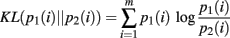
The proposed method combines a spatial data-clustering technique (Dasu et al., 2006, 2009) with a Bayesian estimator of the KL-divergence (Kullback, 1959) between discrete distributions over neural ensemble patterns (Wolpert and Wolf, 1995). The KL-divergence is calculated between pairs of probability distributions which share the same domain. Its output is a positive quantity with values greater than zero indicating the distributions compared are not the same. The efficiency of the KL-divergence for hypothesis testing and classification has been studied extensively (Kullback, 1959; Cover and Thomas, 1991). Here the KL-divergence is used to generate a one-dimensional time-series for tracking changes in the dynamics of the ensemble, relative to statistical null hypotheses about the underlying neural firing rates and pairwise interactions.
To calculate the KL-divergence one must provide a method for transforming the neural ensemble data into a probability mass function. Like others (Schneidman et al., 2006; Tang et al., 2008; Marre et al., 2009), we define a discrete joint distribution over possible ensemble patterns. One consequence of this formalism is that unobserved, but possible, ensemble patterns must be assigned a probability through the use of a prior distribution. The choice of a prior distribution will be expounded below. To keep the prior from unduly influencing our estimates, we use an adaptive quantization scheme to compress the complete set of ensemble patterns into a smaller set of multinomial categories. The data structure used to achieve this compression is the kdq-tree. Originally developed by Dasu et al. (2006) for detecting changes in multi-dimensional, streaming telecommunications data, this data structure aggregates regions of low sample density, and may be thought of as a data-driven binning scheme. Importantly, the kdq-tree was originally developed specifically for cases where the distribution generating the dataset is unknown.
First, samples of ensemble data of equal size, representing the null hypothesis and test data, are filtered through the kdq-tree. Next, the multinomial samples output by the kdq-tree are input to a routine that calculates the Bayesian estimator of the KL-divergence to determine whether the test data conform to the null hypothesis. The time-series of KL-divergence values are then examined for significant deviations from the null hypothesis. Since the null hypothesis is defined by features of the neural ensemble estimated within a previous epoch, significant deviations demarcate changes in these features across time, and therefore changes in the dynamics of the neural ensemble. The processing of ensemble data by this method is schematized in Figure 1A, from conversion of the dataset via the kdq-tree through examining the time-series of KL-divergence values to test the null hypothesis.
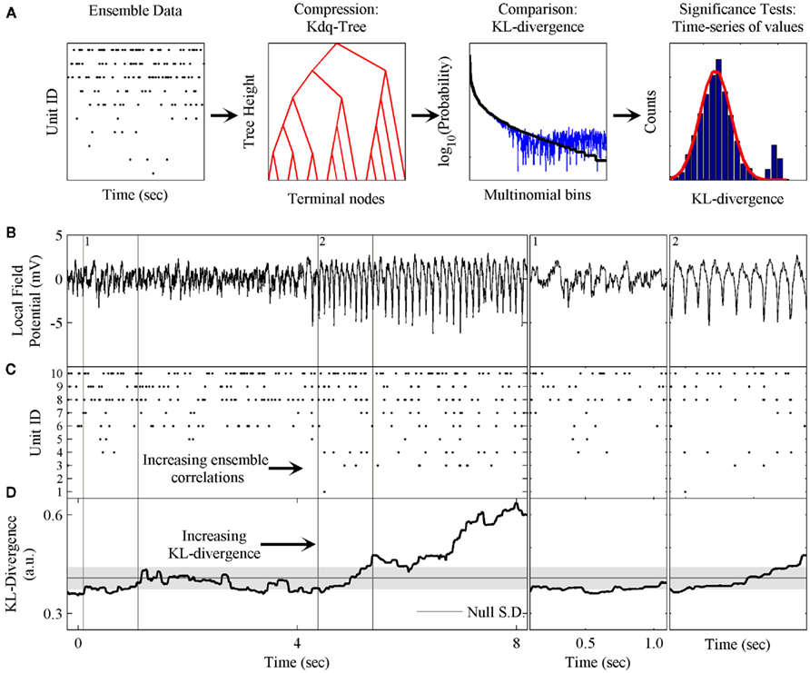
Figure 1. Schematic of method and phenomenon of interest. (A) The components of the method are: the kdq-tree for transforming the ensemble data into multinomial samples; the expected value of the KL-divergence under the Dirichlet posterior distributions on the two multinomial distributions; and the evaluation of the time-series of KL-divergence values to test the null hypothesis. (B) A local field potential recording from the rat somatosensory barrel field (S1bf) exhibiting the μ-rhythm. (C) A simultaneously recorded neural ensemble of 10 units from S1bf. (D) The KL-divergence output of this method, which uses only the ensemble data as input. The shaded gray area indicates the mean ± SD, respectively, of the KL-divergence under the null hypothesis of independence among the neurons. Subpanel 1: A zoomed in example of the background LFP, ensemble activity, and KL-divergence. Subpanel 2: The onset of the μ-rhythm, ensemble data and KL-divergence at higher resolutions. Note the correlations in the ensemble data during the negative phase of the μ-rhythm.
We next provide a detailed exposition of the method. We demonstrate its application and performance upon simulated ensemble data. Furthermore, it will be shown to be capable of detecting changes in the correlation structure of ensemble data missed by firing rate metrics. We conclude by demonstrating its utility upon neural ensemble data collected from awake behaving rodents.
Exposition
Transforming Ensemble Data into a Probability Mass Function
Figure 1 provides an overview of the method and an example of the phenomenon of interest to us. These data were collected from the somatosensory barrel cortex (S1bf) of a behaving rat (unpublished data). Figure 1 shows both local field potential (LFP; Figure 1B) and ensemble data (Figure 1C) collected from a rat’s S1bf. Here we are interested in examining whether the dynamics of the ensemble reflect changes in the LFP. Halfway through the time-series, there is a clear change in the LFP data. This feature is the so-called μ-rhythm commonly observed in idle rats (Semba et al., 1980; Wiest and Nicolelis, 2003; Tort et al., 2010). Figure 1D demonstrates the ability of our method to detect this change in the dynamics of the ensemble data. Subpanels 1 and 2 zoom in on a few cycles of the μ-rhythm to illustrate that this change in the LFP is correlated with a change in the patterns of activity emitted by the ensemble. In particular, the negativity of the μ-rhythm coincides with an increase in the probability of correlated firing among the neurons. The role played by the LFP might just as easily have been a stimulus presentation, a basic motor response, a response signaling a decision or any other variable of interest.
We next illustrate the details of the transformation from ensemble data to probability mass functions. This is done in the context of checking if the results of Schneidman et al. (2006) hold for our ensemble data from S1bf. Here the generalized iterative scaling algorithm (Darroch and Ratcliff, 1972) is used to fit the maximum entropy pairwise model to the transformed ensemble data. Figure 2A shows a typical example of the weak pairwise cross-correlations observed between units within S1bf. For this dataset, the cross-correlation peaks were centered at approximately zero lag and were 20–40 ms wide (the inset of Figure 2A shows the details of an example peak). This is an important piece of experimental information used to set a bin width parameter used to simplify the cross-correlation structure (set to 20 ms here). An alternative is to assume a Markov order and fit a Markov model to the sequence of ensemble patterns (see Marre et al., 2009). This was not done here because the Markov order is a free parameter that vastly increases the complexity of the model. We will show that it is possible to detect subtle changes in the correlation structure of ensemble data using this binning scheme.
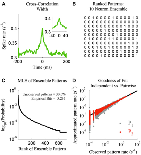
Figure 2. The statistical mechanics description of neural ensemble data. (A) An example of the cross-correlation width observed between neurons recorded from the S1bf. Inset: The peak examined prior to setting a spike bin parameter (20 ms). (B) The 14 most frequent ensemble patterns, from left to right, derived from the 10 unit ensemble. (C) The maximum likelihood estimate distribution of ensemble patterns based upon 2 h of continuous recording. Inset: The amount of missing data for this 1024 pattern system and the entropy of the distribution in bits. (D) The independent (P1) and maximum entropy pairwise model (P2) fits to the dataset in terms of the predicted and actual rate of ensemble patterns.
Another feature of this transformation is the designation of any neural activity within a bin as either active (1) or inactive (0), as opposed to integer spike counts. This simplification loses the information individual neurons transmit via brief bursts of activity, but it allows for a complete description of the distribution of ensemble patterns based solely on the number of recorded neurons. Furthermore, we will show that the information conveyed by these bursts is recoverable by tracking the ensemble firing rate in parallel.
This processing of the ensemble data results in a series of row vectors, one for each time bin, ranging over all possible ensemble patterns, from completely inactive (all 0’s) to maximally active (all 1’s; Figure 2B). The resulting data object is an N × M matrix where N is the number of time bins and M is the number of neurons (For M neurons there are 2M possible ensemble patterns.). The dataset is now a sequence of binary vectors from a discrete M-dimensional space, Y. Let e = {y1, y2,…, yN} be a sample of ensemble data with each yi ∊ Y. The maximum likelihood estimate (MLE) of the probability of observing a given pattern, yi is then:

The operator C(yi/e) counts the number of times ensemble pattern yi appears in the sample. Normalizing these counts to one and ranking them in descending MLE probability determines the probability mass function (Figure 2C).
We now fit maximum entropy models to the MLE probability distribution to test whether these provide a good fit to the ensemble data. First, we fit the independent model, which assumes the probability of observing any ensemble pattern is the product of the probabilities of the individual active and inactive neurons within a pattern. The independent model is calculated as:
Here the Xj designates one of the M neurons in the ensemble and yji indicates the jth component of ensemble pattern, yi. We then fit the pairwise model, which also incorporates the simultaneously observed pairwise correlations. Fitting the maximum entropy pairwise model consists of maximizing the Shannon entropy subject to the constraints that it must be consistent with the expected firing rates and pairwise correlations measured from the dataset:
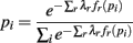
The probability the model assigns to each ensemble pattern is simplified here as pi. The first term on the right of the equals sign is the Shannon Entropy. The first constraint, with parameter λ0, is a normalization constraint and the subsequent sum of constraints, with parameters λr, require the model output match the expectations of these measured quantities, 〈fr(p)〉 (Jaynes, 1957). The form of the resulting model is obtained by setting ∂Q/∂pi = 0 and solving for pi:
The denominator satisfies the normalization constraint, making this model a probability mass function. Figure 2D shows the improved fit of the pairwise model (P2) compared against the independent model (P1) for this, on average, weakly correlated ensemble. This analysis validates the result of Schneidman et al. (2006): a model incorporating the firing rates and pairwise interactions within a neural ensemble does provide a good fit to these ensemble data. Consequently, tracking changes in these features over time provides a good approximation to the dynamics of the ensemble.
To increase our temporal resolution of the dynamics of the ensemble we must make estimates using fewer samples. This introduces a host of issues that must be taken into account. For instance, to our knowledge all analyses of the joint distribution of ensemble patterns (Schneidman et al., 2006; Tang et al., 2008), including our own, observe that the low firing rates of neurons and weak correlations between them result in ensembles rarely if ever producing many of the possible patterns (Figure 2C). Low sample density and outright missing data pose a challenge to any statistical analysis of ensemble data at higher temporal resolutions, because a probability mass must be assigned to all yi ∈ Y. Our solution is to first compress these data into multinomial samples via the kdq-tree and then multiple these by a prior distribution when calculating the Bayesian estimate of the KL-Divergence.
Compression Via the kdq-tree
The kdq-tree is used to compress the ensemble data before multiplying it by a prior distribution. Otherwise maximum-a posteriori estimates of the KL-divergence are liable to be more a reflection of the prior distribution than the dataset (Skilling, 1985). Therefore, to aggregate regions of low sample density, and thereby reduce the influence of the prior distribution, we employ the kdq-tree (Dasu et al., 2006).
The kdq-tree data structure provides a data-driven approach to compressing regions of low sample density that scales linearly in the number of dimensions and data points (Dasu et al., 2006). This makes its use computationally efficient for a wide range of ensemble and sample sizes. The general principle followed by the kdq-tree is to bin finely where data density is high and coarsely where it is low. The parameters of the kdq-tree are an integer that sets the minimum number of data points a bin must contain before it is subdivided, and a real number that sets a constraint upon the width of any bin along any dimension. For ensemble patterns the latter parameter is always set to 1/2 since all dimensions consist of the values 0 and 1. The intuition behind the kdq-tree may be apprehended by representing it as a binary tree data structure (Figures 3A,B).
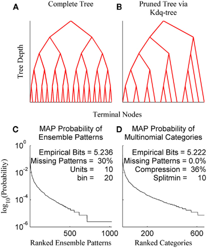
Figure 3. The kdq-tree. The kdq-tree as a binary tree: (A) A simulated ensemble of five variables with sufficient data density to generate the complete tree representing all of the 32 (25) possible ensemble patterns. (B) A simulated ensemble of five variables with insufficient data density, resulting in a pruned tree wherein ensemble patterns with low sample density are aggregated. (C) The maximum-a posteriori probabilities of ensemble patterns for a 10 neuron ensemble recorded in the rat somatosensory cortex. (D) The same data after compression via the kdq-tree. Note there is no longer any missing data.
In Figures 3A,B each fork represents a splitting of a parent node (bin) along a single dimension, and the K leaves of the binary tree are the terminal nodes (the resulting bins). Each node contains the boundaries of a bin and the number of samples contained therein. As one moves down the tree, from top to bottom, the bins get smaller (see Algorithm 1). Figure 3A shows the binary tree representation of a kdq-tree fit to a simulated ensemble of five neurons. In this case, all of the possible 25 = 32 ensemble patterns were visited with sufficient frequency to generate the entire tree (Depth = 5, Terminal Nodes = 32). Figure 3B details a similar binary tree structure, but in this case not all of the ensemble patterns contain enough samples to generate the complete tree, resulting in a pruned tree (Depth = 5, Terminal Nodes = 15). In both examples, this binary tree is constructed iteratively by cycling through each of the five variables in the ensemble and at each step determining whether to split the parent node into two children nodes. This process continues until no node meets the criteria for subdivision set by the parameters. This compression into multinomial samples eliminates missing data, with only a slight loss of empirical entropy (Figures 3C,D: data from an ensemble of 10 recorded neurons). This transformation allows us to track differences in samples of ensemble data as differences in the posterior distributions using the Bayesian estimator of the KL-divergence.
ALGORITHM 1: Construct Binary kdq-tree (data, splitmin)
data should be a binary array of [Ndatapoints by Nvariables];

axis ← 1, the first of Nvariables;

currentnode ← 1;

unused ← 2;

assignednode ← an array of 1’s the size of Ndatapoints;

  INITIALIZE a tree data structure T;

T.Addnode( );

T.parent(currentnode) ← 0;

T.axis(currentnode) ← axis;

while currentnode < unused do

if T.axis(currentnode) > Nvariables then

   noderows ← indices of assignednode that equal currentnode;

   T.nodesize(currentnode) ← size of noderows;

   INITIALIZE T.children as the array [0,0];

   INCREMENT currentnode;

   continue

end if

noderows ← indices of assignednode that equal currentnode;

T.nodesize(currentnode) ← size of noderows;

if T.nodesize(currentnode) > splitmin then

   ω ← indices of data equal to 0 at T.axis(currentnode);

   α ← indices of data equal to 1 at T.axis(currentnode);

   if ω is empty or α is empty then

      INITIALIZE T.children as the array [0,0];

      INCREMENT currentnode;

      continue

 end if

      T.children(currentnode) ← [unused, unused+1];

      T.Addnode( );

      T.Addnode( );

      INCREMENT axis;

      T.axis([unused, unused+1)) ← axis;

      T.parent([unused, unused+1]) ← currentnode;

      assignednode(ω) ← unused;

      assignednode(α) ← unused+1;

      unused ← unused+2;

end if

      INCREMENT currentnode;

end while

return T;
Tracking the KL-divergence
The KL-divergence is defined as:
It is a convex function between probability density functions and is bound between 0, indicating no difference between the distributions, and +∞. It is only defined for the case where the domains of p1 and p2 are the same. We interpret the KL-divergence as the information for discriminating p1 from p2. In general, the KL-divergence from p2 to p1 is not equal to that from p1 to p2. With this in mind, it is important to note that our calculations of the KL-divergence are always relative to a null hypothesis, with the distribution of this null represented by p2.
The Bayesian estimator for the KL-divergence is derived according to the Laplace convolution method (Wolpert and Wolf, 1995), which requires the specification of a prior distribution. Based upon Figure 2C, we know that many of our ensemble states are unlikely to be observed. What we want then is a prior distribution that is minimally informative while being responsive to updates from sparse data. To achieve this end, we chose the conjugate prior for multinomial likelihoods functions, the Dirichlet distribution, and set all the parameters of the distribution equal to 0.5 (Krichevsky and Trofimov, 1981). The first moment of Bayesian estimator of the KL-divergence according to the posterior distributions of p1 and p2 is calculated, and derived in the Appendix (see also Berkes et al., 2011).
Figure 4 details the behavior of the kdq-tree, our choice of prior, and the estimator of the KL-divergence when applied to the output of two simulated 10 unit ensembles. In this case the null hypothesis was that the test samples were all drawn from the same distribution that generated the first 500 samples (note the zero values in Figures 4C,F, which are the samples used for the null hypothesis). The test window of 500 samples was slid one sample at a time, forward in time, over the entire dataset. At each step the test data was processed as described above and the KL-divergence was estimated between the null and test data.
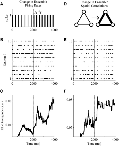
Figure 4. A basic demonstration of the method. (A) Schematic representation of a simulated unit changing its firing rate at sample 2001. (B) A simulated ensemble of 10 variables which all change their firing rates at sample 2001. Firing rates before and after the change were drawn from a distribution generated from ensemble data recorded in the S1bf of five rats. (C) The application of the method to the simulated ensemble. The null hypothesis for the KL-divergence was that these data were all drawn from the distribution that generated the first 500 samples (note the zero values indicate the samples used for the null hypothesis). (D) Schematic representation of three simulated units increasing their pairwise interactions. (E) A simulated ensemble of 10 units that all change their pairwise interactions at sample 2001, while their firing rates remain the same. (F) The method is also able to signal this change in correlations.
These simulations were designed to undergo either a change in firing rates (Figure 4A) or pairwise correlations (Figure 4D) beginning at sample 2001 and persisting through sample 4000. Specifically, in Figure 4B all variables were assigned an initial firing rate and, at sample 2001, each underwent a random change in firing rate (All firing rates were drawn from a distribution derived from unit activity recorded within the S1bf of five behaving rats. All unit waveforms had a signal-to-noise ratio of 4:1 relative to each channel’s background voltage fluctuations, unpublished data.). In Figure 4E, initial firing rates were drawn as in Figure 4B, but here at sample 2001 all variables underwent an increase in pairwise correlations [from correlation(xi, xj) ∼ N(0.005, 0.05) to ∼N(0.8, 0.05)] while firing rates remained the same (the simulation engine of Macke et al., 2009 was used to generate these example data). Figures 4C,F show that the Bayesian estimator of the KL-divergence is able to signal both of these changes.
An examination of Figure 4 illustrates that before applying this method to real data we must derive for the time-series of KL-divergence values a rejection threshold for ruling out the null hypothesis. Specifically, we must provide a means for rejecting the null hypothesis that the KL-divergence matches what one would expect if repeated finite samples were drawn from the null distribution. In Figure 4, this variability is manifest in the behavior of the KL-divergence time-series between samples 1000 and 2000 and again after sample 2501. The magnitude of this variance is a function of the ensemble size, the number of samples within a window, and the null hypothesis considered. We next examine the variance of the null hypothesis en route to defining a rejection threshold for the time-series of the KL-divergence values. We then validate the method’s behavior and performance upon simulated ensemble data for a variety of null hypotheses.
Checking Intuitions and Estimating a Rejection Threshold
To evaluate the behavior of our method, we calculated the expected variance of the resulting KL-divergence for a range of ensemble sizes, sample sizes, and neural features. This was achieved by drawing samples from simulated ensembles generated by stationary distributions. Before estimating the SD of the posterior distribution of the KL-divergence, for multinomial likelihood functions, we derived the second moment of this distribution according to the posteriors of p1 and p2 (see Appendix for details).
The simulation engine of Macke et al. (2009) was then used to generate ensembles of binary variables with mean firing rates and pairwise correlations matched to those observed experimentally. The simulated ensemble data was then binned at 20 ms and the sample size parameter of the kdq-tree was set to five samples. The details of these simulations for varying ensemble and window sizes are shown in Figure 5. Each data point represents the mean ± SD of the KL-divergence. Several important intuitions are apparent from these simulations.
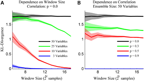
Figure 5. The method preserves intuitions about ensemble data. (A) The variance for draws from a stationary distribution decreases as a function of the size of the sample and the bias increases as a function of the number of neurons within the ensemble. (B) The bias for draws from a stationary distribution decreases with increasing correlations among the variables. Both subplots are mean ± SD of the Bayesian estimator of the KL-divergence.
First, the mean and SD of the KL-divergence is inversely proportional to the window size. Second, the mean is directly proportional to the number of variables in the ensemble (Figure 5A). This means that as the ensemble size increases, relative to the sample size, the likelihood of mistaking pairs of samples from a single distribution for samples from different distributions increases. Alternatively, stationary systems appear more variable if brief observations are made instead longer ones. Third, the mean of our estimates of the KL-divergence are inversely proportional to the degree of correlation among the variables (Figure 5B). In the extreme, if the variables within a system are completely correlated, the distribution reduces to a binomial distribution, greatly reducing the expected KL-divergence. These intuitions are important if we are to differentiate interesting features of the dataset from expected fluctuations in its activity.
It is important to emphasis that the Bayesian estimator of the KL-divergence is positively biased, especially for large ensembles. This is in line with observations made by others about the calculation of Shannon Entropy from ensemble data (Paninski, 2003). This bias is less of a concern for us because we are interested in tracking differences in the time-series of the KL-divergence values, not their absolute values. With these observations in hand, we now estimate the rejection threshold relative to the null hypothesis upon the time-series of KL-divergence values.
Our general goal is to detect epochs in which the dynamics of the ensemble move away from the distribution of the null hypothesis. The calculation of the rejection threshold will depend upon the null hypothesis under consideration. For example, for the null hypothesis of homogeneity among adjacent samples, a surrogate dataset is created by time shuffling the ensemble patterns to break up any temporal structure in the sequence of ensemble data. These surrogate data are then processed according to the method and the mean and SD of the resulting time-series of KL-divergence values are used to set the rejection threshold (see Algorithm 2 for a test of homogeneity among adjacent samples).
Algorithm 2: kdq bayes KL (for homogeneity of adjacent windows)
data: a binary array of [Ndatapoints by Nvariables];

data.sh ← a time-shuffled copy of data (null distribution);

γ: sets the number of data points within a window;

stepsize: sets the number of data points between comparisons;

α sets the value of the parameters of the Dirichlet prior;

T ← Construct Binary kdq-tree (data, splitmin);

i ← 1;

while not at the end of the data do

      Load adjacent samples W1 and W2 of γ samples from data;

      Likewise load W1.sh and W2.sh from data.sh;

      n1 ← multinomial sample generated by filtering W1 through T;

      n2 ← multinomial sample generated by filtering W2 through T;

      n1.sh ← multinomial sample generated by filtering W1.sh through T;

      n2.sh ← multinomial sample generated by filtering W2.sh through T;

      KLs[i+γ-1] ← bayes KL(n1, n2, α);

      KLs.sh[i+γ−1] ← bayes KL(n1.sh, n2.sh, α);

      Slide windows W1, W2, W1.sh and W2.sh by stepsize;

      i ← i+1;

end while

null.mode ← mode(KLs.sh[γ to end- γ by stepsize]);

null.std ← standard deviation(KLs.sh[γ to end- γ by stepsize]);
When considering the null hypothesis of independence among the neurons within an ensemble we generate pairs of surrogate independent samples by shuffling the time indices of each neuron within each window. This preserves the firing rates of all the neurons within the window while disrupting any correlations among them. These data are then processed and the rejection threshold is calculated as above.
Figure 6 details our method’s ability to detect changes in the dynamics of the ensemble data missed by the commonly used population, or ensemble, firing rate metric (Laubach et al., 2000; Friedrich and Laurent, 2001; Dorris and Glimcher, 2004) as well as changes in the correlation structure of an ensemble.
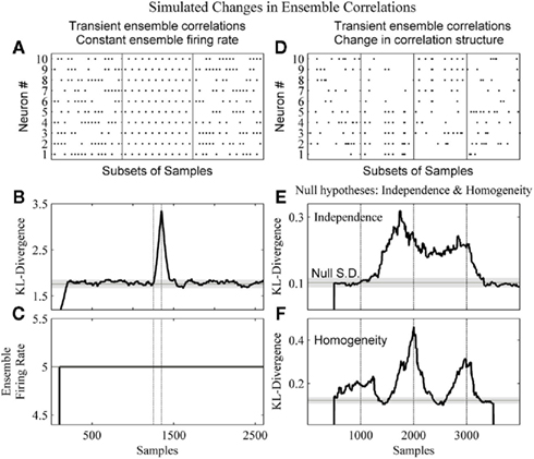
Figure 6. The method detects changes in both the strength and structure of ensemble correlations. (A) A subset of the dataset from a 2600 sample simulated ensemble of 10 units wherein each column sum is equal to 5. In the complete simulation from samples 1251–1350 there is the alternating pattern seen in the middle panel. (B) The resulting KL-divergence after the method was applied to the simulated ensemble. The null hypothesis was stationarity relative to the initial window’s 100 samples. (C) The ensemble firing rate output with a 100 sample running average. (D) A simulated ensemble exhibiting a change in correlation structure. The four subpanels show subsets of 20 samples from epochs of 1000 samples. These epochs were independence, correlation among variables 1–5, correlation among variables 6–10, and independence, respectively. (E) The resulting KL-divergence after evaluating the null hypothesis of independence among the variables. (F) The resulting KL-divergence after evaluating the null hypothesis of homogeneity between adjacent samples. Vertical black lines indicate the beginning and end of sample epochs. The horizontal black line and gray shaded areas indicate the mode and the SD, respectively, of the time-series of the analyses.
In Figure 6A, a simulated ensemble of 10 variables was generated so that the column sum for each sample was constant (five samples). From samples 1251–1350, 100 samples exhibit a stereotyped correlation structure (Figure 6A, middle panel: a subset). This was done to provide an example of a disassociation of a change in ensemble firing rate from a change in ensemble correlations. Our method and the ensemble firing rate were calculated from these simulated data. For both analyses a 1 sample bin and a 100 sample window were used. For the ensemble firing rate this 100 sample window was used to calculate a running average. This matched the time-scales of the analyses. For the kdq-tree, the sample density parameter was set at 5. The null hypothesis tested was homogeneity among samples. The KL-divergence was able to detect this change in the correlation structure (Figure 6B), and by design the ensemble firing rate could not (Figure 6C). In Figure 6D, a simulated ensemble of 10 variables was generated such that they were independent from samples 1–1000, from samples 1001–2000 variables 1–5 were correlated, from samples 2001–3000 variables 6–10 were correlated, and they were all independent again from samples 3001–4000. Here we used a window size of 500 samples. To detect this change in correlation structure using our method, we evaluated two null hypotheses. The first null hypothesis was that the variables were independent (Figure 6E). The second null hypothesis was that adjacent samples were homogeneous (Figure 6F). Figure 6E shows that our method was able to reject the null of independence between samples 1000 and 3000. Figure 6F shows a rejection of the null of homogeneity almost immediately as the leading edge enters the first epoch of correlated data. It then decreases as both windows enter this epoch before increasing again and reaching a maximum around sample 2500, as each of the adjacent windows occupies one of the two differently correlated epochs. Taken together, this demonstrates the ability of our method to detect a change in the structure of neural ensemble correlations.
To demonstrate the performance of our method under difficult conditions, Table 1 details the performance of the complete method at detecting small changes in the degree of correlation among variables. Again, the firing rates of the variables within the simulated ensembles were drawn from an empirical distribution derived from chronic extracellular recordings in five behaving rats (unpublished data). The parameters considered were the number of variables in the ensemble, the window size, the significance level for detection, and the sample density parameter for the kdq-tree. In all cases, 100 epochs of 5500 samples each were generated, and an increase in ensemble correlations from 0 to 0.1 occurred from samples 4501 to 5000. The null hypothesis evaluated was that the samples all came from the same distribution that generated the samples within the first window. The significance level was set relative to the rejection threshold of the null distribution calculated as described above. The confidence interval method of Dasu et al. (2009) was used to mark detections. Detections were marked when the number of significant KL-divergence values within a 100 sample window exceeded the proportion expected by chance. Performance was classified as “Detected,” “Late,” “False,” and “Miss.” A change was logged as “Detected” if the time of detection was within two window lengths of the actual change. Otherwise, any detection outside this interval but before another simulated change in these data was marked “Late.” If the number of detections was greater than the number of epochs, then this excess was logged as “False,” indicating false alarms. If no detection was signaled between two changes, it was logged as a “Miss.”
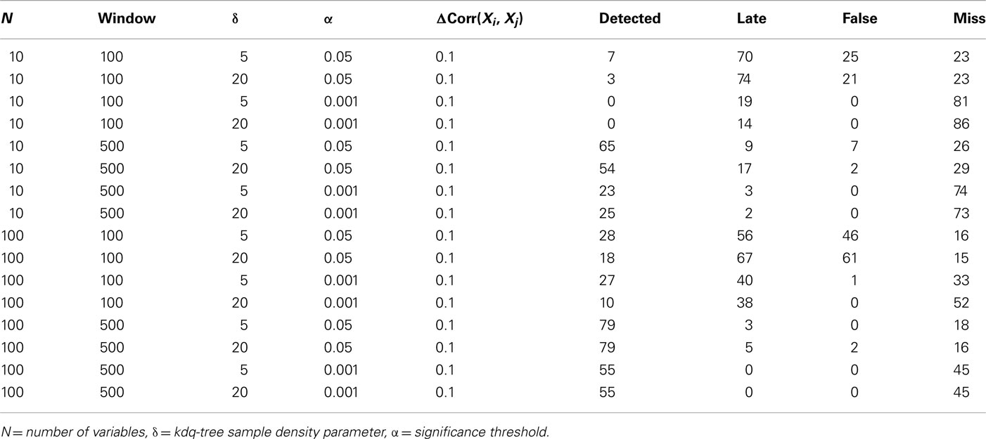
Table 1. Results from simulations designed to evaluate the method’s ability to detect 100 changes in ensemble correlations over a range of parameter values.
The most important result of these simulations is that it is far easier to detect small, widespread changes in the correlations among units within large ensembles than within smaller ensembles. This implies that if small, widespread changes in ensemble correlations are coincident with behavior, then increasing the number of recorded units in combination with this method should increase the ability of experimenters to detect this feature. This point will be considered further in the discussion. From the simulations, it was also clear that matching the window size to the duration of the change increased the number of detections, which recommends considering multiple time-scales when investigating ensemble correlations. As might be expected, increasing the significance level for detection decreased the number of false alarms but increased the number of false negatives. The threshold upon sample density was found to have only a small effect upon detection performance for the range of values considered.
Application to Real Data
Having explicated our method, we now demonstrate its application to real neural ensemble data (Figure 7). Our goal was to detect the occurrence of the μ-rhythm apparent in the LFP using only the ensemble data (Figures 7A,B). To begin, the bin width parameter was set to 20 ms and a window of 200 binned samples was used. For comparison against a comparable estimate of ensemble firing rate, the ensemble data was binned as both binary activations and spike counts. The KL-divergence was set to evaluate the null hypothesis that the neurons within the ensemble fire independently of one another. The kdq-tree was constructed using the complete data sorted in descending order by firing rate (Figure 7B). For the kdq-tree, the integer threshold upon data density was set at five samples. After compression, the resulting multinomial samples were then used to estimate the KL-divergence. The mode ± the SD of the time-series of surrogate KL-divergence values representing the null hypothesis is plotted to mark when the null is rejected (Figure 7D). The mode ± the SD of the ensemble firing rate time-series set the rejection threshold for this estimator (Figure 7C).
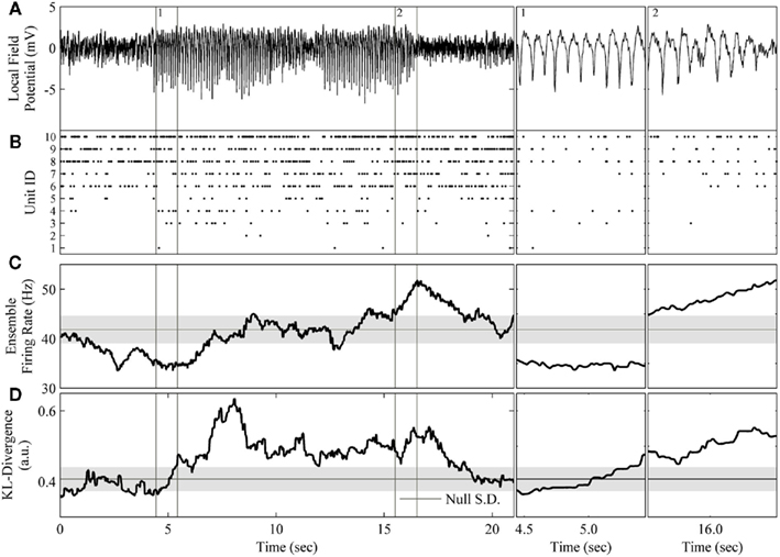
Figure 7. Application of the complete method to the rodent μ-rhythm. (A) One channel of local field potential activity recorded simultaneously from rat S1bf exhibiting two large amplitude bouts of the μ-rhythm. (B) The simultaneously recorded ensemble of 10 units. (C) The ensemble firing rate calculated in a 200 sample window of spike counts binned at 20 ms and slid one sample at a time. (D) The resulting KL-divergence after evaluating the null hypothesis of independence. Subpanels 1: A period at the beginning the μ-rhythm when the correlations among units began to increase. The KL-divergence clearly signals this change while the ensemble firing rate does not. Subpanel 2: A period at the end of μ-rhythm when the correlations among the units reached a plateau followed by a burst of activity. The ensemble firing rate signals the burst of activity. The horizontal black line and gray shaded area indicate the mode and the SD, respectively, of the time-series of the analyses.
The most apparent difference between these analyses is that the KL-divergence was capable of signaling the sustained epoch of increased ensemble correlations (Figure 7D), whereas the ensemble firing rate only clearly signals the tail end of the second bout of the μ-rhythm (Figure 7C). These epochs are of particular interest because they signal a disassociation of changes in pairwise interactions from changes in neural firing rates. Both features detect a decrease in ensemble activity prior to the initiation of the μ-rhythm, but then the KL-divergence signals an increase in correlated activity missed by the ensemble firing (Figure 7, subpanel 1). Interestingly, the cadence of the μ-rhythms coincides with a plateau and subsequent decrease in the KL-divergence, while the ensemble firing rate signals a burst of activity (Figure 7, subpanel 2). An examination of the ensemble rasters validates the description of the dataset provided by these features. The initiation of the μ-rhythm begins with a decrease in ensemble activity followed by an increase in ensemble correlations without an appreciable change in unit firing rates. The bouts of μ-rhythms are then terminated by a burst of activity, which is detected by the ensemble firing rate.
The ability of the proposed method to detect changes in ensemble correlations, in conjunction with the population firing rate’s sensitivity to bursts of activity, paints a rich picture of these data. Moreover, by augmenting this method with the calculation of the ensemble firing rate, the spike count information lost when transforming the ensemble data to generate the joint distribution is recovered. This example shows that tracking both the KL-divergence (Figure 7D) and the ensemble firing rate (Figure 7C) makes it straightforward to disassociate changes in firing rates from changes in the higher order moments of ensemble data. Altogether, our method provides an automated process for generating a succinct summary of neural ensembles dynamics.
Discussion
Contemporary neurophysiological techniques for recording from behaving subjects track the output of ensembles of neurons. Put simply, the ensemble is the set of recorded neurons. This is done with minimal knowledge about the anatomical connections among the recorded neurons or any unobserved inputs that drive them. Until the advent of technology capable of detailing the relevant neural networks in vivo, progress will depend upon the ability of neuroscientists to make sound inferences about the structure and influences upon neural ensemble activity. This is to say, the impressive parametric models that have been developed for describing ensemble interactions (Brown et al., 2001; Truccolo et al., 2005; Eldawlatly et al., 2009) are only as convincing as the experimental evidence which supports them. While the body of work demonstrating some relationship between the structure of ensemble data and behavior is growing (Deadwyler and Hampson, 1997; Durstewitz et al., 2010; Truccolo et al., 2010), the functional significance of transient fluctuations in the dynamics of neural ensembles remains an open question. This led us to develop a computational method that utilizes unsupervised learning algorithms for the purpose of tracking changes in the dynamics of neural ensembles on time-scales comparable with behavior.
Our approach was to synthesize the non-parametric method of Dasu et al. (2006, 2009) with the statistical mechanics description of ensemble data provided by Schneidman et al. (2006). These components were chosen to match well the practice of exploratory data analysis (Tukey, 1962; Mallows, 2006). As such, they are non-parametric and unsupervised, reflecting the fact that the mechanisms generating ensemble data are largely unknown and their covariance with behavior remains to be investigated. The kdq-tree was chosen for its ability to aggregate poorly estimated regions of the data space (Figure 2D). Moreover, because it scales linearly in the number of variables and data points, it is appropriate for a wide range of ensemble and window sizes (Figure 5). Furthermore, the use of the Bayesian estimator of the KL-divergence (Kullback, 1959; Wolpert and Wolf, 1995) provided us with a sound framework for evaluating possible differences between ensemble data sampled over intervals short enough for making comparisons with behavior. Moreover, the Bayesian estimator allowed us to incorporate prior information about the dataset. In particular, the use of the Dirichlet prior with parameters all set to 0.5 biased us toward a sparse posterior over ensemble patterns, in accordance with experimental observations (Figure 2). Together, this allowed us to track changes in the dynamics of ensemble data by inspecting the time-series of the KL-divergence values relative to the corresponding expected variance of the null distribution (Figure 7).
Methods such as principal component analysis (Jolliffe, 2002) and factor analysis (Yu et al., 2009) were not used to reduce the dimensionality of the dataset because of their reliance upon the assumption that these data come from a Gaussian distribution. Because the set of ensemble patterns is unordered, smoothing methods such as kernel density estimation (Rosenblatt, 1956; Botev et al., 2010) would only be appropriate after first selecting an arbitrary ordering of the ensemble patterns. It is worth noting that the order in which the kdq-tree evaluates variables is arbitrary, and other data compression schemes are worth considering if they are well suited to the peculiarities of ensemble data. Moreover, simulations demonstrated the free parameter upon sample density to be rather robust (Table 1). Lastly, the choice to leave the spike bin and window size as user-specified free parameters reflects the view that these require expert knowledge for their specification, and will depend upon the experimental preparation under observation.
The exposition and demonstrations provided herein illustrate our method’s efficacy for evaluating a range of hypotheses about the dynamics of ensemble data. These include detecting changes in the structure of pairwise interactions among neurons within an ensemble, distinct from changes in neural firing rates (Figure 6). Throughout, we made the assumption that the features of interest would manifest as transient changes in the dynamics of the ensemble activity. This reflects that general observation that changes in the dynamics of neural ensembles are observable as transient modulations of neural firing rates and pairwise interactions. On the contrary, one might imagine an ensemble could shift from one sustained equilibrium state to another. Such a change would be clear from an inspection of the times-series of KL-divergence values under the null hypothesis of stationarity and would recommend a partitioning of the time-series of these data prior to further analysis. An alternative to this unsupervised approach would be a supervised learning scheme in which a classifier is built using training data to validate whether some ensemble data carries information about a behavior of interest (Churchward et al., 1997). The KL-divergence has been used extensively for classification (Kullback, 1959) and our method could easily be adapted to such a framework by an appropriate partitioning of the dataset to generate training data for each presumed class.
There are a few differences between our method and those of others, which are both principled and methodological. For instance, analyses such as the ISI distance method of Kreuz et al. (2007) or the gravity method of Lindsey and Gerstein (2006) are designed to detect synchronous events involving subsets of neurons within an ensemble. We did not take this approach for three reasons. First, we wished to avoid treating the recorded ensemble as a neural network, because of the experimental limitations listed above. Therefore, we adopted a framework that is agnostic to whether changes are caused by interactions between the recorded neurons or by unobserved inputs. Second, sets of neurons do not appear to fire in rigid patterns, i.e., sync-fire chains (Abeles, 1982a), but in a stochastic manner amenable to statistical analysis. Third, outside of a few areas within the brain which do show a high degree of synchrony, e.g., CA1 of the hippocampus, there is a paucity of experimental evidence for widespread, strong correlations among neurons in most brain areas. The norm is the observation of weak pairwise correlations (Schneidman et al., 2006; Tang et al., 2008; Shlens et al., 2009). It remains unclear why these periodic synchronizations are not observed at their downstream targets. Is it a due to random delays between the neural oscillator and its target(s)? If so, our method is capable of detecting the influence of such an upstream neural oscillator without having to model the explicit neuron-to-neuron interactions. This could be done by first applying our method to neural ensemble data from the downstream area under the null hypothesis of independence and then comparing the resulting time-series of KL-divergence values to the time-series of the neural oscillator.
Methodologically, by being grounded within the framework of statistical hypothesis testing, our method captures a notion of prior expectation many ad hoc methods lack. Some form of a prior expectation is important when analyzing complex systems, because simple changes in variance can result in incredible variability, producing myriad red herrings. This being said, other methods may be more sensitive to novel patterns of interest in the dataset, and in future work we will extend the set of null hypotheses to include a wider range of neural features. Ultimately, which method will most clearly illustrate the relationship between neural ensemble activity and behavior is an empirical question. In particular, the use of maximum entropy models in neuroscience has been extended to include both temporal interactions among ensemble patterns (Marre et al., 2009) and to argue for higher order correlations in ensemble data (Ohiorhenuan et al., 2010). In addition, a forthcoming extension will calculate the inverse from significant changes in the ensemble dynamics to the best estimate of the set of neurons that contributed to the change.
In conclusion, we presented a flexible method for signaling changes in the dynamics of neural ensemble data on time-scales comparable with behavior. We demonstrated the validity and utility of this method and recommend its use to complement existing analyses. This method is particularly sensitive to widespread, transient fluctuations in the correlations among neurons within an ensemble (Table 1). Importantly, it is capable of disassociating changes in ensemble correlation structure from changes in ensemble firing rate (Figure 6). This makes it an excellent candidate for mining ensemble data in search of evidence for hypotheses ranging from the reader mechanisms governing neural computation (Buzsaki, 2010) to the role of oscillations in the brain (Fries, 2005).
The application left to experimentalists is to observe the covariance between large values of the KL-divergence and other variables of interest. A MATLAB® implementation of this method, along with an addition visualization tool, is available at: http://code.google.com/p/kdq-bayes-kl
Conflict of Interest Statement
The authors declare that the research was conducted in the absence of any commercial or financial relationships that could be construed as a potential conflict of interest.
References
Abeles, M. (1982b). Quantification, smoothing, and confidence limits for single-units’ histograms. J. Neurosci. Methods 5, 317–325.
Abeles, M., Bergman, H., Gat, I., Meilijson, I., Seidemann, E., Tishby, N., and Vaadia, E. (1995). Cortical activity flips among quasi-stationary states. Proc. Natl. Acad. Sci. U.S.A. 92, 8616–8620.
Averbeck, B. B., Latham, P. E., and Pouget, A. (2006). Neural correlations, population coding and computation. Nat. Rev. Neurosci. 7, 358–366.
Berkes, P., Orbán, G., Lengyel, M., and Fiser, J. (2011). Spontaneous cortical activity reveals hallmarks of an optimal internal model of the environment. Science 331, 83–87.
Botev, Z. I., Grotowski, J. F., and Kroese, D. P. (2010). Kernel density estimation via diffusion. Ann. Stat. 38, 2916–2957.
Brown, E. N., Nguyen, D. P., Frank, L. M., Wilson, M. A., and Solo, V. (2001). An analysis of neural receptive field plasticity by point process adaptive filtering. Proc. Natl. Acad. Sci. U.S.A. 98, 12261–12266.
Churchward, P. R., Butler, E. G., Finkelstein, D. I., Aumann, T. D., Sudbury, A., and Horne, M. K. (1997). A comparison of methods used to detect changes in neuronal discharge patterns. J. Neurosci. Methods 76, 203–210.
Cover, T. M., and Thomas, J. A. (1991). Elements of Information Theory. New York, NY: Wiley-Interscience.
Darroch, J., and Ratcliff, D. (1972). Generalized iterative scaling for log-linear models. Ann. Math. Stat. 43, 1470–1480.
Dasu, T., Krish, S., Venkatasubramanian, S., and Yi, K. (2006). “Detecting changes in multi-dimensional data streams,” In 38th Symposium on the Interface of Statistics, Computing Science, and Applications (Interface ’06), Pasadena, CA.
Dasu, T., Krishnan, S., Lin, D., Venkatasubramanian, S., and Yi, K. (2009). “Change (detection) you can believe in: finding distributional shifts in data streams,” in Proceedings of the 8th International Symposium on Intelligent Data Analysis: Advances in Intelligent Data Analysis VIII IDA ’09 (Berlin: Springer-Verlag), 21–34.
Deadwyler, S. A., and Hampson, R. E. (1997). The significance of neural ensemble codes during behavior and cognition. Annu. Rev. Neurosci. 20, 217–244.
Dorris, M., and Glimcher, P. (2004). Activity in posterior parietal cortex is correlated with the relative subjective desirability of action. Neuron 44, 365–378.
Durstewitz, D., Vittoz, N. M., Floresco, S. B., and Seamans, J. K. (2010). Abrupt transitions between prefrontal neural ensemble states accompany behavioral transitions during rule learning. Neuron 66, 438–448.
Eldawlatly, S., Jin, R., and Oweiss, K. G. (2009). Identifying functional connectivity in large-scale neural ensemble recordings: a multiscale data mining approach. Neural Comput. 21, 450–477.
Friedrich, R. W., and Laurent, G. (2001). Dynamic optimization of odor representations by slow temporal patterning of mitral cell activity. Science 291, 889–894.
Fries, P. (2005). A mechanism for cognitive dynamics: neuronal communication through neuronal coherence. Trends Cogn. Sci. (Regul. Ed.) 9, 474–480.
Ghahramani, Z. (1998). “Learning dynamic Bayesian networks,” in Adaptive Processing of Sequences and Data Structures, eds C. L. Giles and M. Gori (Salerno: Springer-Verlag), 168–197.
Jones, L. M., Fontanini, A., Sadacca, B. F., Miller, P., and Katz, D. B. (2007). Natural stimuli evoke dynamic sequences of states in sensory cortical ensembles. Proc. Natl. Acad. Sci. U.S.A. 104, 18772–18777.
Kreuz, T., Haas, J. S., Morelli, A., Abarbanel, H. D. I., and Politi, A. (2007). Measuring spike train synchrony. J. Neurosci. Methods 165, 151–161.
Krichevsky, R., and Trofimov, V. (1981). The performance of universal encoding. IEEE Trans. Inf. Theory 27, 199–207.
Kullback, S. (1959). Information Theory and Statistics (Dover Books on Mathematics). Mineola, NY: Dover Publications.
Laubach, M., Wessberg, J., and Nicolelis, M. A. L. (2000). Cortical ensemble activity increasingly predicts behaviour outcomes during learning of a motor task. Nature 405, 567–571.
Lindsey, B. G., and Gerstein, G. L. (2006). Two enhancements of the gravity algorithm for multiple spike train analysis. J. Neurosci. Methods 150, 116–127.
Macke, J. H., Berens, P., Ecker, A. S., Tolias, A. S., and Bethge, M. (2009). Generating spike trains with specified correlation coefficients. Neural Comput. 21, 397–423.
Marre, O., El Boustani, S., Frégnac, Y., and Destexhe, A. (2009). Prediction of spatiotemporal patterns of neural activity from pairwise correlations. Phys. Rev. Lett. 102. Available at: http://view.ncbi.nlm.nih.gov/pubmed/19392405
Nicolelis, M. A. (ed.). (2008). Methods for Neural Ensemble Recordings, 2nd Edn. Boca Raton, FL: CRC Press.
Nicolelis, M. A. L., Dimitrov, D., Carmena, J. M., Crist, R., Lehew, G., Kralik, J. D., and Wise, S. P. (2003). Chronic, multisite, multielectrode recordings in macaque monkeys. Proc. Natl. Acad. Sci. U.S.A. 100, 11041–11046.
Ohiorhenuan, I. E., Mechler, F., Purpura, K. P., Schmid, A. M., Hu, Q., and Victor, J. D. (2010). Sparse coding and high-order correlations in fine-scale cortical networks. Nature 466, 617–621.
Palm, G., Aertsen, A. M. H. J., and Gerstein, G. L. (1988). On the significance of correlations among neuronal spike trains. Biol. Cybern. 59, 1–11.
Rosenblatt, M. (1956). Remarks on some nonparametric estimates of a density function. Ann. Math. Stat. 27, 832–837.
Schneidman, E., Berry, M. J., Segev, R., and Bialek, W. (2006). Weak pairwise correlations imply strongly correlated network states in a neural population. Nature 440, 1007–1012.
Semba, K., Szechtman, H., and Komisaruk, B. R. (1980). Synchrony among rhythmical facial tremor, neocortical “ALPHA” waves, and thalamic non-sensory neuronal bursts in intact awake rats. Brain Res. 195, 281–298.
Shlens, J., Field, G. D., Gauthier, J. L., Greschner, M., Sher, A., Litke, A. M., and Chichilnisky, E. J. (2009). The structure of large-scale synchronized firing in primate retina. J. Neurosci. 29, 5022–5031.
Sivia, D. (1996). Data Analysis: A Bayesian Tutorial (Oxford Science Publications). Oxford, UK: Oxford University Press.
Suner, S., Fellows, M. R., Vargas-Irwin, C., Nakata, G. K., and Donoghue, J. P. (2005). Reliability of signals from a chronically implanted, silicon-based electrode array in non-human primate primary motor cortex. IEEE Trans. Neural Syst. Rehabil. Eng. 13, 524–541.
Tang, A., Jackson, D., Hobbs, J., Chen, W., Smith, J. L., Patel, H., Prieto, A., Petrusca, D., Grivich, M. I., Sher, A., Hottowy, P., Dabrowski, W., Litke, A. M., and Beggs, J. M. (2008). A maximum entropy model applied to spatial and temporal correlations from cortical networks in vitro. J. Neurosci. 28, 505–518.
Tort, A. B. L., Fontanini, A., Kramer, M. A., Jones-Lush, L. M., Kopell, N. J., and Katz, D. B. (2010). Cortical networks produce three distinct 7-12 Hz rhythms during single sensory responses in the awake rat. J. Neurosci. 30, 4315–4324.
Truccolo, W., Eden, U. T., Fellows, M. R., Donoghue, J. P., and Brown, E. N. (2005). A point process framework for relating neural spiking activity to spiking history, neural ensemble, and extrinsic covariate effects. J. Neurophysiol. 93, 1074–1089.
Truccolo, W., Hochberg, L. R., and Donoghue, J. P. (2010). Collective dynamics in human and monkey sensorimotor cortex: predicting single neuron spikes. Nat. Neurosci. 13, 105–111.
Wiest, M. C., and Nicolelis, M. A. L. (2003). Behavioral detection of tactile stimuli during 7-12 Hz cortical oscillations in awake rats. Nat. Neurosci. 6, 913–914.
Wolpert, D. R. (1996). “Determining whether two data sets are from the same distribution,” in Maximum Entropy and Bayesian Methods 1995, eds K. Hanson and R. Silver (Kluwer Academic press).
Wolpert, D. H., and Wolf, D. R. (1995). Estimating functions of probability distributions from a finite set of samples. Phys. Rev. E 52, 6841–6854.
Yu, B. M., Cunningham, J. P., Santhanam, G., Ryu, S. I., Shenoy, K. V., and Sahani, M. (2009). “Gaussian-process factor analysis for low-dimensional single-trial analysis of neural population activity,” in Advances in Neural Information Processing Systems 21, eds D. Koller, D. Schuurmans, Y. Bengio, and L. Botton (Cambridge, MA: MIT Press), 1881–1888.
Appendix
In this appendix the Bayesian estimator for the first and second moments of the KL-divergence over discrete distributions is derived according to the method of Wolpert and Wolf (1995). This appendix is meant to stand alone and so some of the results of Wolpert and Wolf (1995) are recapitulated. The interested reader should consult the original work of Wolpert and Wolf (1995).
The original result of Wolpert and Wolf (1995) was derived for a single, discrete distribution. When applying this method to derive the Bayesian estimator for the KL-divergence it is necessary to consider two discrete distributions, which share the same domain. This extension has been demonstrated for a quadratic loss function in “Determining Whether Two Data Sets Are From The Same Distribution” by Wolpert (1996).
Preliminaries
We are interested in using a data set n to estimate some function of a probability distribution Q(p). To estimate Q(p) from the data n we must first determine the probability density function P(p|n). We know that we are working with multinomial samples here, so by Bayes’s theorem P(p|n) is given by
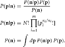
Note that because of cancelation, the constant  does not appear in P(p|n). Thus,
  . Therefore, the kth order moment of Q(p) given n is (∫dpQk(p) P(p|n). If we define
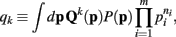
then the kth moment of Qk(p) may be expressed as qk/q0.
In the following, for simplicity P(p) will be assumed to be uniform, i.e., P(p) ∝ ∆ (p)Θ(p), where Θ(p) = Πiθ(pi), the Heaviside theta function, Δ(p) ≡ δ(Σi pi − 1), and the proportionality constant is set by the normalization condition ∫dpP(p) = 1.
When deriving the Bayesian estimator for the KL-divergence we utilize a Dirichlet prior, 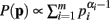 for Re(αi) > 0.
Lastly, to be consistent with the notation of Wolpert and Wolf (1995) we define
I[,] is a functional of its first argument and a function of its second argument.
Recapitulation of Derivations by Wolpert and Wolf (1995)
In Theorem 1 it is shown that if a function H(p) factors as  then the general form of the integral ∫(dp H(p)Δ(p)Θ(p) is that of a convolution product of m terms.
Define the Laplace convolution operator ⊗ by
Theorem 1. If  then
then
Proof. The pi may not be independently integrated since the constraint  exists. This constraint is crucial for deriving the closed form solution, and is reflected in the explicit definition of the integral
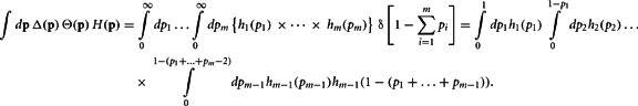
Define the m variables τk, k = 1,…, m, recursively by  and τk ≡ τk − 1 − pk − 1. Since
 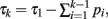 our integral may be rewritten as

Now, with the definition of the convolution, the integral can be rewritten as

Since the convolution operator is both commutative and associative, we can repeat this procedure and write the integral above as
Q.E.D.
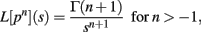
Theorem 2 restates the important Laplace Convolution Theorem. The Laplace transform operator L is defined as 
Theorem 2. If L[hi(pi)] exists for i = 1,…, m, then 
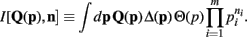
Theorems 1 and 2 allow for the calculation of integrals of the form I[Qk(p), n] for functions Q(p) that may be factored as 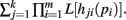 Both the Shannon entropy and the KL-divergence may be factored in this manner.
Theorem 1 and 2 may be used in concert to calculate the normalization constant I[1, n]. It will be shown that manipulating I[1, n] provides the base for deriving the Bayesian estimator for the KL-divergence. The derivations require the Gamma function Γ(z) given by Γ(z) =  for Re(z) > −1.
Theorem 3. If Re(ni) > −1 ∀i = 1, …, m, then 
Proof. For the integral  , the hi(pi) are given by
Since
we have, by Theorems 1 and 2
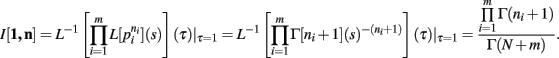
Q.E.D.
When deriving the Bayesian estimator for the KL-divergence we will need to calculate variants of integrals of the form  The key to these derivations is the fact that
 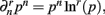 which immediately leads to the following.
Theorem 4. For Re(ni) > −1 ∀i,

The justification for the interchange of the derivative and integral is provided in Appendix C of Wolpert and Wolf (1995). In using Theorem 4, note that since  we have
  .
.
Following the notation of Wolpert and Wolf (1995) we define Φ(n)(z) = Ψ(n − 1)(z) and ∆Φ(n)(z1, z2) ≡ Φ(n)(z1) − Φ(n)(z2), where Ψ(n)(z) is the polygamma function 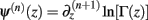 and
and 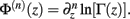
Theorem 5. For Re(ni) > −1 ∀i,
Proof. 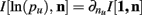 (by Theorem 4). Substituting the result from Theorem 3 for I[1,n] above we have
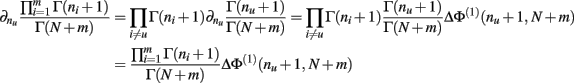
Q.E.D.
Theorem 6. For Re(ni) > −1 ∀i,
Proof. Similar to, but far more laborious than, the proof of Theorem 5. This proof is not detailed here.
Novel Derivation of the Bayesian Estimator for the KL-Divergence
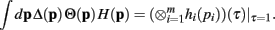
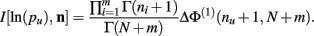
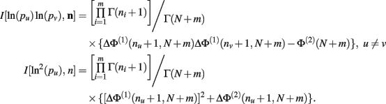
The derivation of the first and second moments for the KL-Divergence according to the Laplace Convolution method of Wolpert and Wolf (1995). We consider a system of m possible states and an associated vector of m probabilities for those states  For two multinomial samples, let the total number of count across states be N for each sample and denote the vectors of state counts by nj = (nj(i)), 1 ≤ i ≤ m, j = {1,2} and
  Here we define the KL-divergence as:
The derivation requires the evaluation of the following integrals:
As above, the derivation follows from modifying an analogously defined I[1, n1, n2] term through the repeated application of Theorem 6. Here
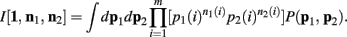
One notable difference here is the fact that we don’t just consider uniform priors. The α parameters reflect our choice of a Dirichlet prior, which is simply incorporated into this framework as “pseudo-counts” upon the states.
Below is for the case α1(i) = α2(i) = α, ∀i. Since p1 and p2 are independent, Theorem 3 above allows us to calculate the integral of I[1,n1, n2] as
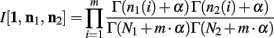
The ∆Φ(i) and Φ(i) functions are defined as in Wolpert and Wolf (1995).
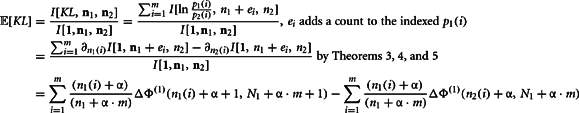
The second moment requires the repeated application of Theorems 5 and 6. This is clear from the expansion of the square of the KL-divergence.
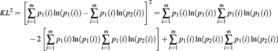
Now we can calculate the integral for the individual components of this expansion as
Q.E.D.
Reference
Keywords: neural ensemble data, spikes, local field potential, data analysis, KL-divergence
Citation: Long II JD and Carmena JM (2011) A statistical description of neural ensemble dynamics. Front. Comput. Neurosci. 5:52. doi: 10.3389/fncom.2011.00052
Received: 01 February 2011;
Accepted: 01 November 2011;
Published online: 28 November 2011.
Edited by:
Nicolas Brunel, Centre National de la Recherche Scientifique, FranceReviewed by:
Maneesh Sahani, University College London, UKEhud Kaplan, Mount Sinai School of Medicine, USA
Copyright: © 2011 Long II and Carmena. This is an open-access article subject to a non-exclusive license between the authors and Frontiers Media SA, which permits use, distribution and reproduction in other forums, provided the original authors and source are credited and other Frontiers conditions are complied with.
*Correspondence: John D. Long II, Helen Wills Neuroscience Institute, University of California Berkeley, 754 Sutardja Dai Hall, MC #1764, Berkeley, CA 94720, USA. e-mail: jlong29@gmail.com