An instruction language for self-construction in the context of neural networks
- Institute of Neuroinformatics, University of Zürich / Swiss Federal Institute of Technology Zürich, Zürich, Switzerland
Biological systems are based on an entirely different concept of construction than human artifacts. They construct themselves by a process of self-organization that is a systematic spatio-temporal generation of, and interaction between, various specialized cell types. We propose a framework for designing gene-like codes for guiding the self-construction of neural networks. The description of neural development is formalized by defining a set of primitive actions taken locally by neural precursors during corticogenesis. These primitives can be combined into networks of instructions similar to biochemical pathways, capable of reproducing complex developmental sequences in a biologically plausible way. Moreover, the conditional activation and deactivation of these instruction networks can also be controlled by these primitives, allowing for the design of a “genetic code” containing both coding and regulating elements. We demonstrate in a simulation of physical cell development how this code can be incorporated into a single progenitor, which then by replication and differentiation, reproduces important aspects of corticogenesis.
1. Introduction
Humans have learned to construct complex artifacts using a method in which the components of the target object, and the relations between them, are carefully specified in an abstract “blueprint.” This blueprint is then transformed into instructions that co-ordinate the actions of human or mechanical constructors as they assemble the target from a store of supplied components. Biology, by contrast, has evolved an entirely different approach to the construction of complex systems. Biological systems construct and configure themselves by replication and differentiation from a single progenitor cell; and each cell generates locally its own supply of construction components. One of the most impressive feats of biological construction is the mammalian brain, particularly the neocortex whose information processing is crucial for intelligent behavior. Understanding the principles whereby these cortical circuits construct themselves is crucial to understanding how the nervous system configures itself for function, and these principles could also offer an entirely new approach to the fabrication of computing technologies.
There is substantial literature that considers various kinds of systems that assemble, organize, or construct themselves (Turing, 1952; Von Neumann and Burks, 1966; Whitesides and Grzybowski, 2002; Freitas and Merkle, 2004; Rothemund et al., 2004). We will be concerned only with self-construction as opposed to self-assembly. “Self-assembly” and “self-organization” describe processes through which a disordered system of pre-existing components form organized structures or patterns as a consequence of specific, local interactions among the components themselves (Whitesides and Grzybowski, 2002; Cook et al., 2004; Halley and Winkler, 2008), based on relatively simple construction information. By contrast, “self-construction” in the sense of (Von Neumann and Burks, 1966) means that agents engaged in self-construction use a program-like abstract set of rules to locally direct their own growth and reproduction in the context of locally detectable information present in a pre-existing or self-generated environment. In the biological case, self-construction arises out of the interplay between agents (cells) that express physical function, and the information (genome) that encodes their function.
The relationship between genetic encodings and expressed function has been extensively explored through evolutionary algorithms, which permute abstract code in search of suitable phenotypic function (Toffoli, 2000). Recent work shows how such search methods can be augmented by a more programmatic approach (Doursat, 2008). However, the principles by which a complex functional system can be systematically elaborated from a single precursor cell are much less well understood.
In this paper we strive to simulate directly the self-construction of a complex neuronal network such as the neocortex. The neocortex arises by a complex process of replication, differentiation, and migration of cells (Rakic, 1988, 1995). In this way the initial precursors expand to form a stereotypical laminated plate-like structure composed of about 1011 neurons intricately wired together using a limited number of stereotypical connection patterns (Binzegger et al., 2007).
During the past decades there has been a rapid expansion of the available data describing various aspects of this process. However, the many interactions among the replicating and differentiating cells quickly become intractable to unaided human comprehension. Computational simulation (van Ooyen, 2011) can be a tool for extending our comprehension: by casting development into a simulation, it becomes possible to examine systematically the relationship between the local behavior and interactions of the various cell types, and the final architecture; and so to determine the principles that guide biological self-construction. But the biological data available are so numerous, and yet so incomplete, that they are difficult to comprehend and even simulate fully in their biological detail. Instead, one requires a suitable abstraction of the relationship between the instantiated cellular processes and the genetic information on which these processes depend. This abstraction should be sparse enough to be theoretically interesting, but detailed enough to capture the nature of the biological process.
In this paper we propose such a framework. It is based on a set of primitive instructions, representing basic cellular actions, which can be combined to form networks of instructions of increasing complexity. Most of these networks, or as we call them, “machines,” do not exist initially in an active form. For them to become active, they have to be instantiated (just like a gene has to be expressed, to produce a protein which can bring a new functionality to a cell). Under appropriate conditions, specific machines can instantiate further new machines from their descriptions in the genetic code, or can remove active machines. These principles allow for the expression of cell functionalities such as migration or neurite sprouting, at a specific time in response to specific signals. We call this instruction language “G-code,” since it corresponds abstractly to the genetic code of the cells in our simulations.
In the following sections we describe each of these primitives, and explain how they can be combined to form higher-level functions. We then present examples of typical neuronal behaviors of increasing complexity (chemo-attraction, axonal, and dendritic branching, as well as cell division and differentiation). Finally, we show how to use these neuronal behaviors as building blocks for the self-construction of a target neural network in simulation.
To perform the simulations presented in this work we have implemented a version of the G-code using the software package CX3D (Zubler and Douglas, 2009), which provides a general platform for designing various models of neural development. The actual implementation within this specific simulator are not essential to the presentation of the concepts of the G-code. Implementation details are listed in Section “Materials and Methods.”
2. Results
2.1. Defining Primitive Actions
The G-code is based on a set of 11 primitives, each representing an elementary cell function (Table 1). The list begins with move, the primitive corresponding to the displacement of a soma or a growth cone. secrete and detect are also obvious requirements in the context of biological development; they account for the production and detection of signaling molecules. Since a cell must express many different functions in various combinations during its lifetime, it needs the ability to recruit new machines (active intracellular agents) and to destroy existing ones. This flexibility is provided by the primitives instantiate and kill.
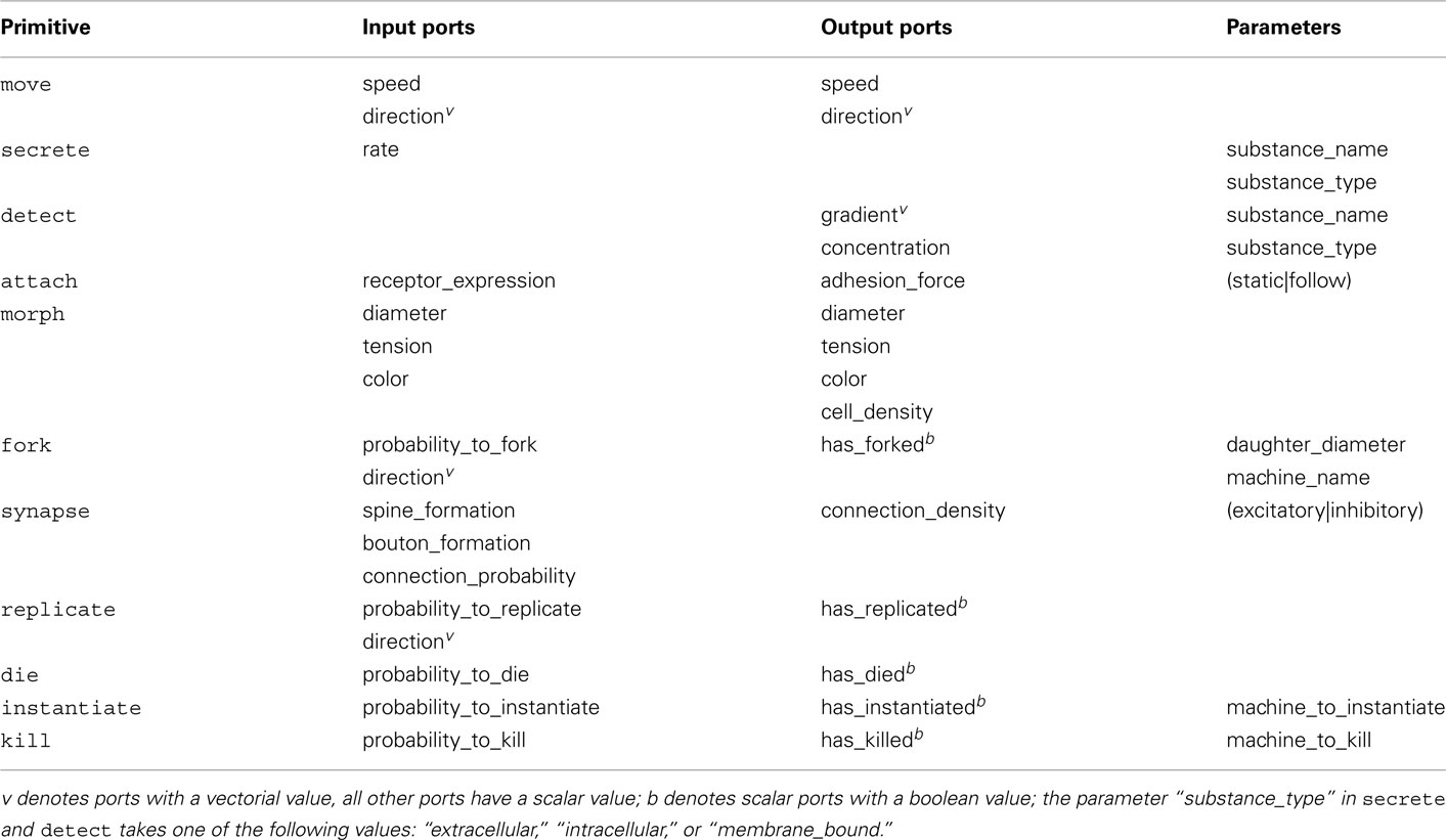
Table 1. Primitives of the G-code, representing atomic cellular behaviors, with their input/output ports and parameters.
In a bio-inspired scheme, the various machines interact as a community of agents enclosed within a cell membrane. In order for these communities to grow in number and specialize in function, they must be able to trigger cell division (including the copying of the G-code genome into the newly formed daughter cells) and cell death. These two additional primitives we term replicate and die. Note that die suppresses an entire cell and destroys the community of agents currently active within this cell, and so differs from kill, which destroys only specific agents (machines) within a cell.
Two more primitives are included to enable the whole cell to interact physically with the environment: morph changes the mechanical properties of a cell segment (e.g., its diameter, inner tension, etc.), while attach sets the level of adherence between a cell and the extracellular matrix, or between two cells. And finally, there are two primitives that produce neuron-specific behaviors: fork causes neurite sprouting and branching; and synapse establishes the pre- and post-synaptic structures required for specialized intercellular communication.
Most of the primitives take parameters that define the context of the action to be taken. For instance secrete and detect take as parameters the name of the substance the actor should secrete or detect, and also the location of the actor (extracellular, membrane bound, or intracellular).
To express an action, a cell must instantiate an active instance of the primitive (or a higher-level machine composed of primitives) by transcription from the appropriate region of its G-code. The resulting primitive (or machine) is localized in a specific discrete cell compartment, such as the soma or a neurite segment. These arrangements are consistent with observations that different parts of a neuron can execute different tasks simultaneously (Polleux et al., 2000), and – at least for a limited amount of time – independently (Davis et al., 1992; Campbell and Holt, 2001). Several instances of the same primitive can co-exist in the same neural segment (for instance two detect primitives, each one allowing for the detection of a different signaling molecule).
2.2. Combining Primitives into Functional Machines
In metabolic pathways, different proteins can act on each other, performing modifications such as methylation or phosphorylation. These actions can be abstracted as a directed graph whose vertices are the various protein types, and whose edges represent the signal transmission effected by the protein-protein interactions (Berg et al., 2011). Our primitives can be organized in a similar manner. Each primitive has one or more input and output ports. Instances of primitives can be connected by linking an output port of one to an input port of another. Input ports are used to induce an action, or modify the modalities of an action, whereas output ports present information on the current state of the element. For instance, the input port “speed” of move, specifies the speed at which a cell element should move, whereas its output port “speed” delivers information about its actual speed (these two values can be different, for example when physical obstacles prevent a desired movement from occurring). Most of the ports transmit or accept a scalar quantity; a few of them transmit or accept a vector. Scalar output ports connect only to scalar input ports, and vectorial output ports only to vectorial input ports.
In biochemical networks, signal propagation is often organized by scaffolding proteins, which can influence both the intensity and the duration of a signal (Kolch, 2005; Locasale and Chakraborty, 2008). Similarly, we allow a set of filters and logical functions that modify the (scalar or vectorial) signals exchanged between primitives (Table 2).
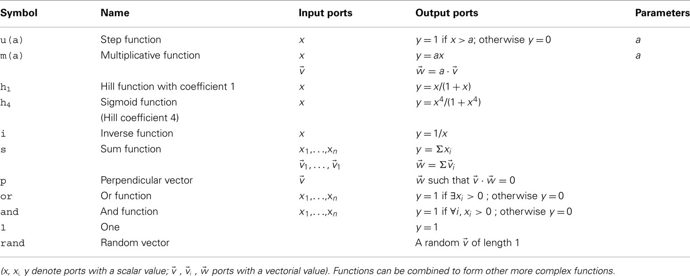
Table 2. Filters and logical functions implemented in the G-code, with input/output ports and parameters.
An assembly of primitive instances providing a complex function is a G-machine. Machines may also have input and output ports (which are the ports of elements contained within the machine that are declared as accessible from outside). These ports allow machines to be connected to primitives or other machines. These arrangements permit machines to be embedded within one another (see below).
As a first example, consider M1, a G-machine that effects chemo-attraction during axonal elongation (see Figure 1A). For biological axons, the sequence can be summarized as follows: membrane receptors detect the presence of specific extracellular signaling molecules, and activate an intracellular signaling cascade, which reorganizes the cytoskeleton and results in a growth cone movement (Wen and Zheng, 2006). To implement this behavior with our framework the “gradient” output port of detect is linked to the “direction” input port of move. The name X and the type e (extracellular) of the signaling molecule to be detected are passed to detect as parameters, detect(X,e). In principle, X will only exist in the extracellular space if somewhere in the space there is a secretor of X.
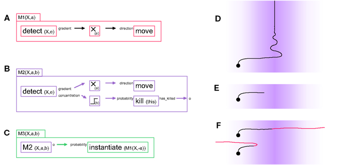
Figure 1. Three “G-machines” used for axon guidance. (A) The machine M1 contains two primitives and one filter, connected by two links: a detect primitive senses the presence of the chemical “X” in the extracellular environment and outputs the gradient of concentration of X via one of its output ports to a filter (which multiplies its input by the scalar factor a). The modified gradient vector is then fed into a move primitive via the input port “direction,” influencing the movement’s direction. When expressed in a cell element, this machine moves the cell element in the direction of the concentration gradient of the signaling molecule X. (B) The machine M2 contains all the elements of M1, with in addition a mechanism to kill (i.e., remove) itself when the concentration level b of the chemical X is reached. This condition is coded with the output port “concentration” of the detect primitive linked to a thresholding filter; the removal of the machine is executed by the primitive kill. M2 has an output port, which outputs a 1 just before the machine removes itself; this output is crucial for sequential actions, as illustrated in the next machine. (C) At instantiation time, the machine M3 contains two elements: an active instance of an M2 machine and an instantiate primitive. Initially M3 acts like its internal M2, i.e., it moves up the gradient of chemical X. But when the internal M2 removes itself, this triggers the instantiation of an M1 machine in which the multiplication factor of the internal filter has the opposite sign. (D) Effect of the machine M1 in simulation when instantiated into an axonal tip (background color intensity proportional to the concentration of the signaling substance X). (E) Effect of M2 in simulation. (F) Effect of M3 in simulation. For illustrative purposes the axon turns red when the internal M2 is replaced by the negative M1. Depending on the value of the threshold b, the axon either does or does not cross the barrier formed by the peak in concentration of chemical X.
This same machine can be converted to perform chemorepulsion rather than attraction by inserting a multiplying filter m(a), which multiplies the vectorial value transmitted between the two primitives by the scalar value a. If a > 0, the machine moves up the concentration gradient of X; if a < 0 it avoids the substance. The machine M1(X,a) contains three elements (two primitive instances and one filter instance) and two links; it has two parameters (X, the name of the signaling molecule it responds to, and a, the filter parameter):
M1(X,a) = {detect(X,e).gradient} → m(a).
→ direction.move}
This “diagrammatic” representation of a machine is used here to give an intuition of the G-code. (Input ports are written to the left of primitives, and output ports to their right.) A more formal definition of a machine is given below.
2.3. Genome and Formal Machine Definition
The “genetic code” (G-code) that is inserted into the precursor cell consists of a list of machines with their names and descriptions. Similar to gene expression, the expression of a G-machine consists of the instantiation of an active machine based on its description in the code. This expression is controlled by the primitive instantiate, which takes the name of the machine to be instantiated as a parameter. Since multiple instances of the same machine can be present in the same cell-element, each machine instance is identified by a unique instance name. Removal of an existing active machine is achieved by the primitive kill, which takes as its parameter the name of the machine instance to be removed. This mechanism resembles the degradation of a local protein “tagged” by ubiquitin proteins. After destruction, a machine can always be re-instantiated later, since its description remains in the G-code.
For their representation in the genome, we define a machine as the quadruple:

where ℐ is the set of input ports of ℳ, 𝒪 is the set of output ports of ℳ, ℰ is the set of machine elements (primitives, filters, or machines) of ℳ, and ℒ is the set of links (pairs of input and output ports of elements of ℰ).
This formal definition of machines offers a way to quantify the complexity of the genetic code, by counting the elements and links of each machine listed:

where α is the coefficient for elements and β a coefficient for links (in principle we use α = 1, β = 0.5).
According to the formal definition (1), the machine performing movement based on extracellular cues described earlier is: M1(X,a) = {{ϕ}, {ϕ}, {detect(X),m(a),move}, {(detect(X,e).gradient, m(a)), (m(a), direction.move)}}. The complexity of M1 is 3 + 2(0.5) = 4.
For brevity we will often use in the remainder of this paper a less formal machine description, of the type {e1 → e2 → … → eN; d1 → d2 → … → dM}, where ei and dj are machine elements connected in chains, and → indicates a link.
2.4. Chemo-Attraction and Midline Crossing
We now illustrate the removal and instantiation of machines in the context of more complex models of chemo-attraction. Because it does not contain a stopping mechanism, the simple machine M1 described above continues its movement indefinitely (Figure 1D). M2 (Figure 1B) has a slightly more elaborated behavior, in that movement ceases once the attractor concentration exceeds a given threshold. M2 combines the displacement principle described in M1 with a mechanism to deactivate itself based on the signaling molecule’s concentration. This behavior is achieved by using the “concentration” port of detect and transmitting this scalar value to the input port “probability_to_kill” of a kill primitive, which will remove the machine and so stop the axonal elongation. We use a threshold filter between these two primitive instances to set precisely the concentration at which the machine is to be killed.
M2 has an output port o that provides an exit status. It outputs the value 1 when the machine deactivates (i.e., removes) itself, and 0 otherwise. This type of output is useful for sequential instantiation of machines during complex developmental sequences.
Note that an equivalent machine M2’ could be constructed, in which an instance of M1 is embedded as an internal machine responsible for the movement, and then independently a chain {detect → threshold → kill → o} could be used for the deactivation of the entire M2’, and for signaling that the machine has been removed.
M1 and M2 can be used to design a simple model of axonal midline crossing, in which an axon is initially attracted by a signaling molecule and then repelled by the same substance, with the concentration of the molecule as the trigger for the switch between these two behaviors (see Figure 1C).
This machine contains an instance of M2 with a positive filter parameter a, and therefore initially moves toward the highest concentration of X. After it has reached the concentration threshold b, the M2 instance removes itself. When it does so, it activates the instantiation of an M1 instance with a negative filter parameter. This results in turning a chemo-attractant signal into a chemo-repellant signal. The threshold b must be set to an appropriate level so that the change of machine does not occur too far from the midline (see Figure 1F). By choosing another parameter for the internal M1 we can also implement the situation where the attracting and repelling signals are mediated through different molecules (Yang et al., 2009).
2.5. Branching Patterns
In addition to elongation and path finding, neurons must regulate the branching behavior of their neurites to form specific axonal and dendritic patterns. This behavior is controlled by the primitive fork. The effect of this primitive depends on its location within the cell: in the soma, it extends a new neurite; in a non-terminal neurite segment it triggers the extension of new side-branches; in a terminal segment it triggers the bifurcation of the growth cone (and thus the creation of two new neurite branches). Each newly created branch is an autonomous cell compartment, which requires its own characteristic machine(s) to be instantiated. fork takes as arguments the machine(s) to be instantiated in each of the new branches that it creates. Thus fork is an implicit call to instantiate, but it also performs the structural changes to the soma or axon. For neurite extension from the soma or side branch formation from a pre-existing neurite segment, fork contains only one set of arguments; in the case of bifurcation at the tip of an elongating neurite, two sets of arguments, one for each daughter branch (the two can be identical for symmetrically behaving branches, or they can be different).
If a machine contains a fork that instantiates an instance of the same type of machine in a new branch, then a recursive branching mechanism is obtained. For instance:
M_branching = {move; 1 → m(p) → probability..
fork(M_branching, M_branching)}
This machine contains a move primitive that elongates the neurite (since the move primitive does not receive an input through its “direction” port, the elongation movement is a “smoothed” random walk – see Materials and Methods). Independently, it contains a branching mechanism that triggers a bifurcation with a probability p. the probability is implemented by a function element that constantly outputs the value 1, linked to a filter that multiplies its input by the constant p. This value is then fed into the primitive fork. After bifurcation, a copy of the same machine is re-instantiated within the daughter branches, so that the process continues indefinitely.
To terminate the branching process, we propose a stopping mechanism in which the elongating machine removes itself with a probability depending on the neurite’s diameter. The diameter can be reduced during elongation or at branch points. The effects of these two mechanisms for diameter reductions are illustrated in the machine M4(a,b) (see Figure 2A), where a is the parameter for reduction during elongation, and b the parameter for reduction at a branch point. The first case is implemented by feeding the current speed into the input port “diameter” of a morph primitive (this input specifies the change in diameter – and not merely the diameter). For the second mechanism, we simply use the parameter “daughter_diameter” of fork. If b ≫ a, the number of branch points on the path connecting the soma to the extremities will be the same, regardless of the actual path length (Figure 2B), whereas if a ≫ b, the path length from the soma to all distal extremities is the same, regardless of the number of branch points (Figure 2C).
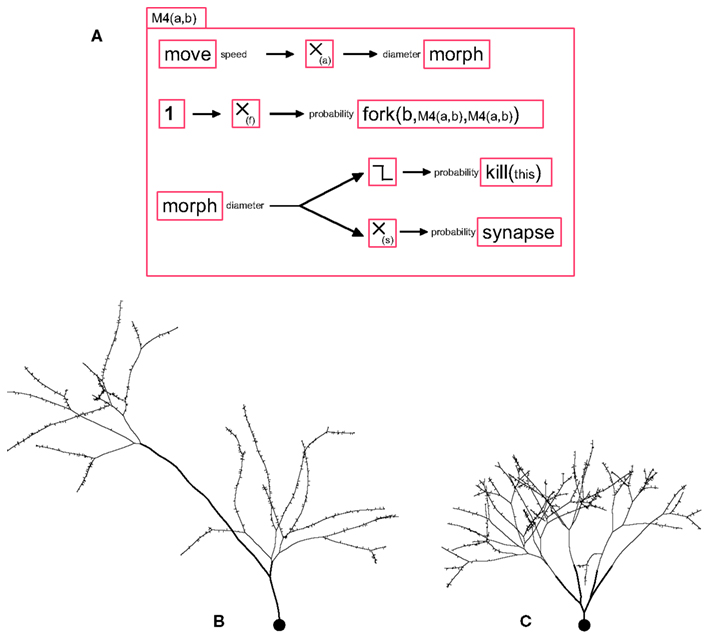
Figure 2. A G-machine capable of producing various branching patterns, with synapse formation. (A) The machine M4 contains four independent processes. (i) A move primitive elongates the neurite, and transmits the current speed to a filter where it is multiplied by the coefficient a, and fed into a morph for diameter reduction (proportional to the distance traveled). (ii) With a probability f, a fork element triggers a neurite bifurcation, producing two daughter branches with diameters smaller than the mother branch’s diameter by a factor b, and instantiates in each of them a copy of the machine M4. (iii) When the diameter falls below a certain limit, a kill primitive removes the machine. (iv) A synapse primitive produces pre- or post-synaptic processes with a probability inversely proportional (proportionality constant s) to the branch diameter. (B) When the diameter is decreased at the bifurcation points but not during elongation, the path from every branch tip to the soma passes the same number of branch points, regardless of the actual length. Note the spines are produced with a density inversely proportional to the neurite diameter. (C) When the diameter is only decreased during elongation and not at branch points, each branch tip is at the same path length from the soma.
Alternative branching mechanisms from the literature are also easily implemented. For example, in a production-consumption model (Kiddie et al., 2005) an intracellular resource substance Y is produced at the soma at a constant rate, and diffuses intracellularly along neurites. The growth cones need this resource for elongation, and they move at a speed proportional to the concentration of the resource substance in the distal element. However, the growth cones consume the resource proportional to how much they have actually elongated. Thus, the limited amount of resource limits the neurite outgrowth. This mechanism is specified as follows:
M_soma = {secrete(Y,i)} in the soma, andM_growth_cone = {detect(Y,i).concentration →
speed.move; move.speed → m(a) → secrete(Y,i)}
in the terminal elements of the neurites, with a being a negative number (negative secretion being equivalent to consumption). It is of course also possible to have the branching probabilities depend on intracellular concentrations. Note that if the substance Y diffuses purely passively within the neuron, there is no need to define a machine for its transport.
2.6. Synapse Formation
Synapse formation is an important part of neural development; not only because the synapses convey electrophysiological activity across the neuronal network, but also because there is a tight interplay between synaptogenesis and the formation of the axonal and dendritic trees. In our framework the primitive synapse regulates three different aspects of synapse formation: the production of a pre-synaptic terminal; the control of the density of post-synaptic elements; and the establishment of a functional synapse between existing pre- and post-synaptic structures. Each of these aspects corresponds to a specific input port. The output port of synapse reports the local density of connections made by a cell element. It can be used for instance to prevent retraction of branches that have already formed synapses.
For example, we observe in pyramidal neurons that the bouton (pre-synaptic terminal) density is higher on terminal branches of the axon, which have a smaller diameter, than on the main shafts (John Anderson, Personal Communication). The implementation of such a mechanism is straightforward: Msynapse(s) = {morph.diameter → m(-s) →bouton_formation.synapse}. The effect of this machine is illustrated in Figure 2.
2.7. Cell Cycle
Cell division is encoded in G-code by the primitive replicate. The original cell divides, forming two daughter cells (by default each with half the mother cell’s volume) each one containing a copy of the genome. In biology this division is regulated by the cell cycle, a sequence of events by which the DNA is first copied and the cell actually divides. The cell cycle is under the control of several proteins that activate and deactivate themselves in a complicated cascade, which is repeated for each division. Several mathematical models of this have been published (see (Fuss et al., 2005) for a review). A simple cell cycle can be achieved with a G-machine containing only three primitives (Figure 3A). It is based on the following principle: as long as the machine is active, the cell will divide as soon as it grows large enough, i.e., if the cell exceeds a certain volume (as reported by the output port “volume” of the morph primitive).
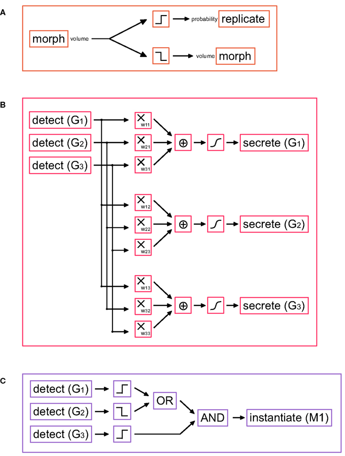
Figure 3. G-machines necessary for cell division and differentiation. (A) Simple cell cycle model: if the soma volume is large enough, the cell divides; otherwise the soma volume is slowly increased. (B) Schematic representation of a small gene regulatory network (GRN), in which three genes G1, G2, and G3 influence each others’ expression. The gene expression is done with the primitive secrete. The production rate is a function of the weighted sum of the concentrations of all three genes (determined with the primitive detect). The same machine can be extended to an arbitrarily large number of genes. (Filters used: multiplication, sum, and Hill function). (C) Example of a read-out gene, which instantiates a machine under certain conditions on the GRN gene concentrations (Filters used: threshold functions, OR, AND).
If the cell is too small, it simply increases its volume (an action controlled via the input port “volume” of morph). To stop the cell cycles (for instance in differentiating neurons) the cell cycle machine is killed. A multiplicative filter can be inserted to regulate the change of volume, and hence the cell cycle speed. We could also combine an input depending on some extracellular or intracellular substance. Based on this idea, we have also implemented a particularly elegant model proposed by Tyson (1991) (see Materials and Methods).
2.8. Gene Regulatory Network
Different cell types express different genes. In biology, the gene expression depends on transcription factors (TFs), small regulatory elements that bind onto specific regions of the genome (the promoter regions) and either activate or suppress the translation of specific genes. Since the TFs are usually themselves proteins, their concentrations are also regulated by gene expression. Several genes coding for TFs and influencing each other’s expression form a gene regulatory network (GRN; Levine and Davidson, 2005). The activity of the different genes of the GRN also influence the transcription of other genes coding for functional or structural proteins (such as those forming the cytoskeleton for instance). In the following, the genes that are regulated by the GRN without being part of the GRN themselves, are termed read-out genes.
Several models of GRNs have been proposed (Schlitt and Brazma, 2007; Karlebach and Shamir, 2008). Our model consists of a set of differential equations describing how the activity gi of each gene (i.e., the concentration of the protein it is coding for) changes depending on the activity of all of the genes in the GRN, for instance through a weighted sum of all activities with a non-linearity:
where gi(t) is the activity of the i th gene, f is a sigmoid function and k a degradation constant (Vohradsky, 2001).
We explain now how a GRN and read-out mechanisms can be expressed in G-code. An important difference from biology is that our GRN and read-out “genes” are seen as machines (since they are composed of primitives and filters) and not as a part of the genome (although the genome contains a description of them). The GRN and the read-out “genes” have thus to be instantiated to become active, and can also be removed.
In our models the TFs are represented as intracellular signal substances. The left hand side of Eq. 3 corresponds to the production rate of the TF coded by the gene i and is implemented using the secrete primitive. The right hand side, representing the effect of various TFs on the promoter regions, is realized by a network of detect primitives, and filters (Figure 3B).
Read-out machines are composed of detect and instantiate primitives. detect primitives are organized in a decision tree that recognizes whether the cell is in an appropriate state (i.e., whether the correct pattern of TFs exists) for triggering the expression of a target gene; instantiates are responsible for the production of the required machines from their G-code description (Figure 3C).
During cell division, the different TFs can be distributed asymmetrically to the two daughter cells, so defining new (and possibly different) internal states. This asymmetrical repartitioning of gene activity permits the formation of different types of cells (see Materials and Methods).
2.9. A Simulation of Cortical Development
Having described some examples of how neural developmental mechanisms can be cast as G-code machines, we now describe how these machines can be customized and combined into longer developmental sequences, and so permit the design of genetic programs for the growth of a wide range of neural architectures, beginning from a single progenitor cell. We illustrate this procedure by growing a cortex-like structure containing three layers (L1, L2, and L3), with one cell type per layer. The goal is to grow the network depicted in Figure 4A: L1 cells send their axons down to the basal dendrites of the L2 and L3 cells; L2 cells project to the basal dendrites of L3 cells; L3 cells project up to the dendrites of the three different cell types. Note that this architecture does not correspond to any real cortical structure; we use it as a didactical example on how to explicitly design a genome to construct a target network.
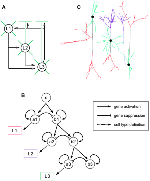
Figure 4. Building blocks for the three-layered cortex simulation. (A) Schematic representation of the desired cortex, with three layers L1, L2, and L3. Axonal projections are depicted by a black arrow, apical and basal dendrites are depicted in green. Note that L1 cells have no apical dendrite. (B) Gene regulatory network (black) and read-out genes (colored) producing the different neuronal types. The main motif is a pair of self exciting, mutually inhibiting genes. When sufficiently expressed, the gene ai induces cell differentiation, whereas bi allows the further division of the progenitors. Each pair is expressed sequentially. (C) Simulation snapshot of the three cell types. Identically colored segments are grown by instances of the same machine (black: axonal shaft, red: axonal ramification, light blue: apical dendritic shaft, violet: apical dendritic tuft, green: basal dendrite).
The first step is the production of the cells. This is achieved by incorporating into the G-code a cell cycle machine, as well as a description of the various cell types. In this example we use the cell cycle model of (Tyson, 1991) described in the Section “Materials and Methods.” For sequentially selecting cells that will become the neuron precursors (in the following order: first L1, then L2, and finally L3), we use the gene regulatory network represented in Figure 4B (see also Materials and Methods). Its main motif is a pair of self enhancing, mutually inhibiting genes. Initially only one gene is expressed (S, for start). During this period a pool of precursors is formed (through symmetrical division, i.e., where each daughter cell is similar). When a specified expression level is reached, S triggers the expression of the genes A1 and B1. The expression product of these two genes is distributed asymmetrically at division, so that some daughter cells will receive more A1, and the others more B1. This differential expression is further increased by the mutual inhibition between these genes. The cells in which the A1 expression reaches a specified threshold will differentiate into L1 cells. The other cells continue to divide and express the next pair of competing genes (A2 and B2), which in turn determine the cells becoming L2 neurons or continuing to divide further and become L3 cells. To recognize the specific gene-expression patterns that define the three cell-types, we incorporate three read-out genes that will instantiate cell type specific cell machines when high levels of A1, A2, or A3 concentrations are reached.
Once a cell is committed to a specific neuron type, it is required to migrate to its final location, so contributing to the formation of a specific layer. For this purpose, the first machine instantiated by the read-out genes is a migration machine, which drags its cell up the gradient of a specific signaling molecule. The migration mechanism is similar to the M2 machine as described in Figure 1. In addition, the read-out genes kill the cell cycle machine (which prevents the further division of the neuron) as well as the GRN and all of the read-out genes: since in this particular model the role of the GRN and the read-out genes is only to define the different cell types, they can be removed to improve the simulation speed. In alternative models we could have the GRN and read-out genes further determine the cell properties; in this case they would remain active or would be re-instantiated at a later point.
Once the neuron precursors have reached their final position, they must extend their axonal and dendritic trees. For this task we include in the genome cell-type specific forking machines which will produce the appropriate neurites, namely: the basal dendrites (common to all three cell types); the main shaft of the apical dendrite (in L2 and L3 cells); and the main shaft of the axon (present in all cells, but with different parameters). The terminal segment of each neurite contains its own independent machine. The ones in the basal dendrites follow a random direction, and are rapidly killed with a probability depending on the (linearly reducing) diameter (using M4, see Figure 2). The axonal and dendritic shafts move toward their target layer, guided by the concentration gradient of the layer-specific signaling molecules. Once they enter a region where the concentration of the molecule they are sensitive to is high enough, the elongation machine kills itself and instantiates a branching machine for the formation of an axonal or dendritic patch (an M2 linked to an M4). The axonal shaft of the L1 cell also contains an additional machine that makes a side branch when the growth cone enters L2, and instantiates in it an axonal patch machine. Figure 4C shows a grown instance of each cell-type, color-coded by the machines used for each cell part. Note that the machines can be used in more than one cell type (e.g., the basal dendrite machine is used in L1, L2, and L3).
The G-code to generate this neural network contains the description of 17 different machines (Table 3). When inserted into a single progenitor cell, the first machine (main) is instantiated. This machine instantiates the cell-cycle, the GRN, the three read-out genes, and an internal clock (constant production of an intracellular substance), and so launches the growth process (Figure 5).
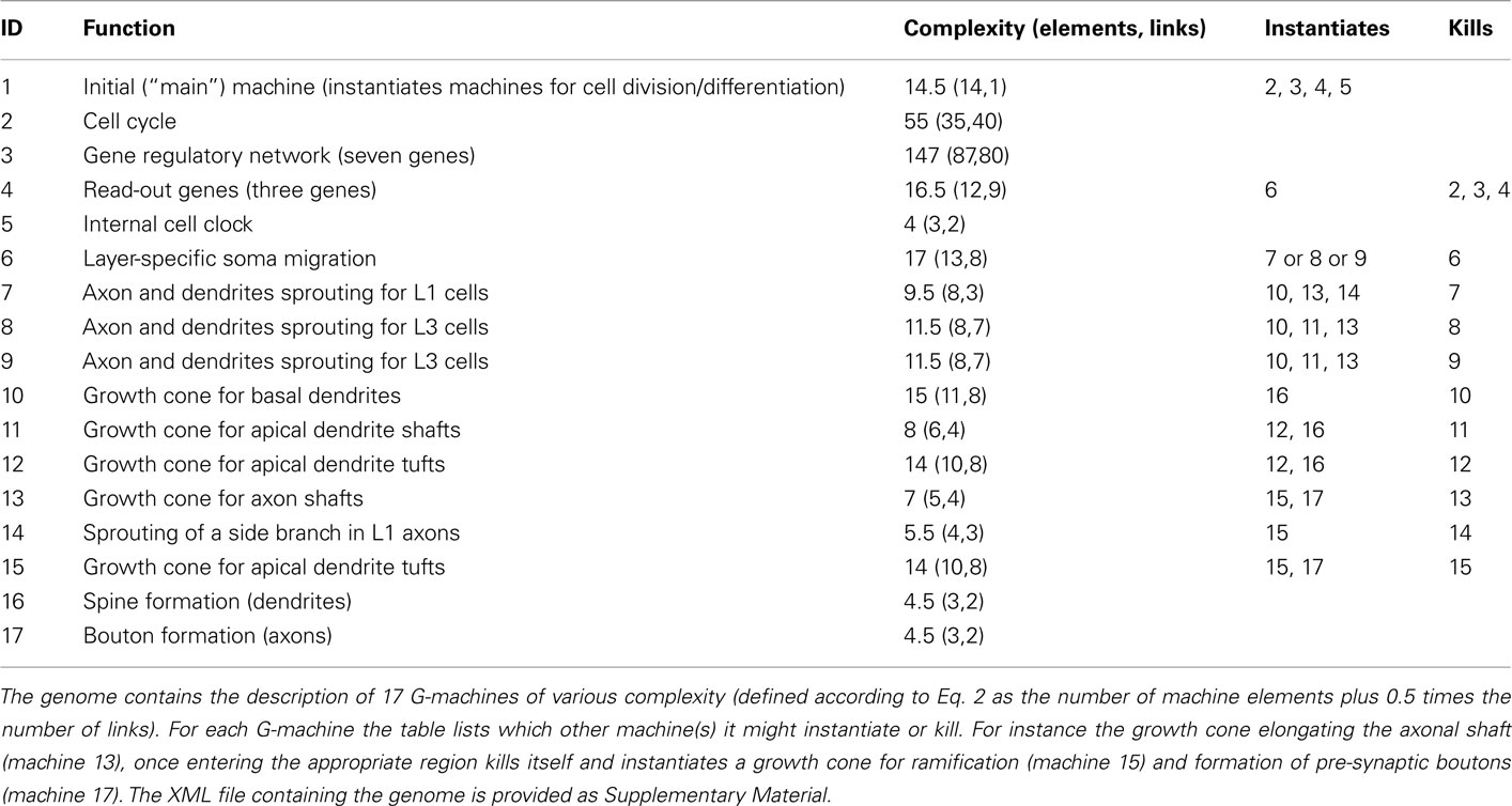
Table 3. Overview of the genome used for the construction of the three-layered cortex (see Figure 5).
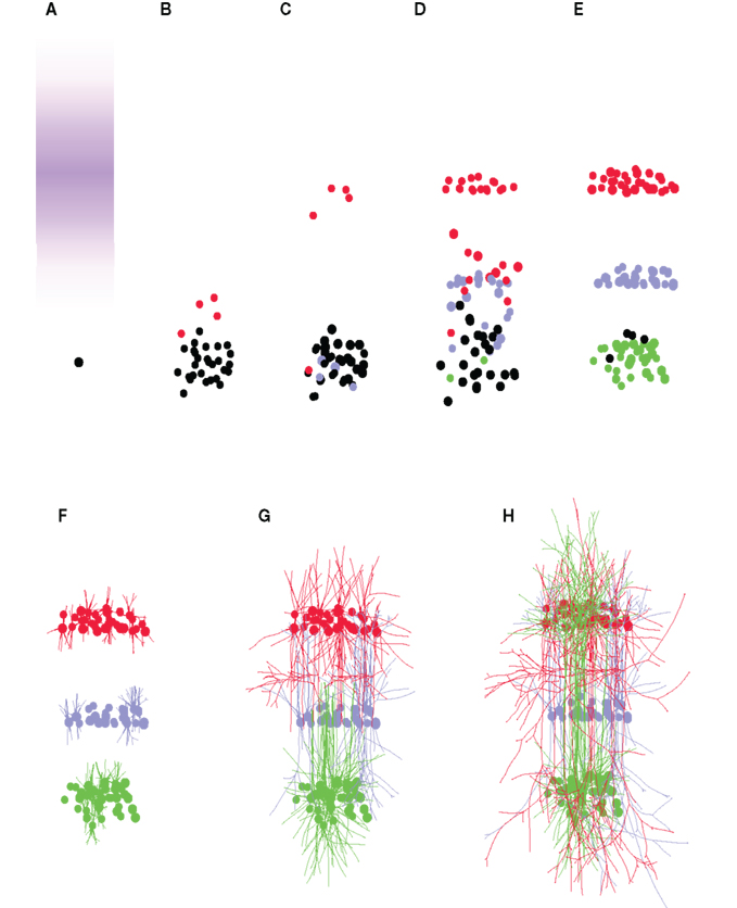
Figure 5. Formation of a three-layered cortex. (A) The simulation starts with a single precursor cell (black). Three signaling molecules “L1,” “L2,” and “L3” define three different areas (for clarity, only the concentration of “L1” is shown in violet). (B) The precursor divides, forming a precursor pool, from which some cells differentiate into L1 cells (red). (C) L1 cells quit the cell cycle, and migrate up the gradient of the “L1” signaling substance, forming the first neuronal layer. L2 cells start to be formed as well (blue). (D) The last L1 cells migrate to their layer. L2 and L3 (green) cells are produced, and settle into the region with the highest concentration of their associated chemical. (E) The last precursors turn into L3 cells. (F–H) When the layers are in place, neurons complete their differentiation by growing axonal and dendritic processes in a layer-specific manner. In total, 89 cells were produced from the first precursor cell (for clarity, only one quarter of the cells have their neurites shown).
3. Discussion
G-code is a framework for directing the self-construction of neural networks in a biologically plausible manner. As such, it offers a tool for understanding the principles of biological development. It is based on a small set of primitives that represent elementary intracellular and cellular functions. These primitives can be combined into functional networks that we call “G-machines,” similar to biochemical pathways, and capable of reproducing complex developmental patterns. We have shown how a description of these machines can be encoded in an efficient way in a text file (for instance with an XML format, see Materials and Methods) that serves as the complete genetic code for developing neural tissues in simulation.
Over the past few decades several groups have explored the use of genetic encodings for the generation of artificial neural networks. The earliest works employed rather explicit coding schemes that used a direct mapping of the genotype onto the phenotype, such as a chromosome describing the neural connectivity matrix (Jian and Yugeng, 1997). Such an explicit encoding of a weight matrix is biologically implausible, and has the inconvenience that the length of the genetic code increases quadratically with network size. Grammar-based models such as L-systems circumvent this scaling problem: simple rules can give rise to extremely complicated networks (Kitano, 1990; Boers et al., 1993; Vaario and Shimohara, 1997). But they too lack biological plausibility in that they do not tend to model the actual growth of a neural structure (Nolfi, 2003) and are context insensitive. More plausible models have offered gradient-based growth of specific connections between neurons (Rust et al., 1996), cell division, and migration (Cangelosi et al., 1994; Kitano, 1995); and have incorporated a gene regulatory network (GRN) for orchestrating neuronal growth (Eggenberger, 2001).
Most approaches have used evolutionary algorithms to search for a genome that encodes a suitable neural network, often with the motivation to use the network to control a co-evolved virtual creature (Sims, 1994; Schramm et al., 2011). This approach is useful for finding genomes that satisfy specific fitness criteria, but it provides little understanding of the principles of self-construction, in the sense that a genome that is suitable for one task, cannot be directly modified to solve a different task. Moreover evolutionary search does not scale well with problem size: Impractically large computational resources would be required to search for the genome able to generate realistically sized cortical circuits. A more explicit design strategy is called for.
There have been a few attempts to explicitly design a genetic code that grows a desired network, without relying on an evolutionary algorithm. Gruau et al. (1995) described a graph grammar for automatic construction of abstract networks. Doursat (2008) has proposed growth systems in which abstract cells proliferate and form patterns on a lattice; the fate of these cells is determined by an internal gene regulatory network. Roth et al. (2007) proposed a more biologically realistic model of development for a multicellular organism with a simple neural system, capable of performing a foraging task. Zubler and Douglas (2010) introduced a coding scheme for controlling the growth pattern of individual simulated neurites.
To formalize the relation between the genetic information and developmental patterns we have presented an instruction language based on 11 primitive neural actions. Of course, each primitive represents an extremely complex mechanism, that might involve hundreds of different proteins. However, our intention here was not to model the detailed biophysics of the neurons, but rather to understand the interaction between inert encoded mechanism and its spatio-temporally ordered expression as functioning intracellular machines. Therefore we have allowed ourselves a certain level of abstraction. The set of primitives would change if we decided to increase the level of details at a molecular level, in which case we would have primitives describing the polymerization and depolymerization of microtubules for instance.
The contribution of this paper is to offer a framework allowing the explicit programming (Nagpal, 2002) of a genetic code for growing a desired neural architecture in biologically plausible way, without relying on an evolutionary algorithm. The procedure includes the following steps. (1) Using a cell cycle machine, and a mechanism to produce the desired quantities of different cells. (2) Decomposing the desired dendritic and axonal arbors of each cell type into distinct regions, and designing a G-machine for growing each one of these regions. (3) Linking the machines in chains of expression [with removal of machines after completion of dedicated tasks, while launching the next machine(s)]. This approach appears to scale favorably. For example, adding new cell types, or designing a more complex branching pattern for one particular cell type is not detrimental to the rest of the code: adding new machines does not perturb the functioning of the existing ones. And since the G-code is modular (the same machine can be expressed in different cells, higher-level machines can contain other machines etc.), pieces of the genome can be re-used in different cells.
Our intention here was not to demonstrate the full capabilities of the G-code, but to explain it in a didactical way; therefore the examples presented are simple. In particular the three-layered cortex presented has limitations as a model of cortical development. The major one is that it develops in a pre-labeled environment, which seems to contradict the principles of self-construction. Another limitation is the limited number of layers and cell types, as well as the simplified architecture of the cells. However, we have previously shown (Zubler and Douglas, 2009) how to produce a laminated cortical structure in an unprepared environment, and how to make layer-specific branching patterns in CX3D. We are now implementing these more biologically plausible procedures in G-code, and will soon present them in the context of a large-scale simulation of cortical development.
3.1. Complexity
In the three-layered cortex example, 60% of the genetic code is used for the generation of the three cell sub-populations (cell cycle: 15.3%, GRN: 41%, read-out genes with promoters: 4.6%); whereas the extension of the axonal and dendritic arbors only represent 40% of the genome (see Table 2). At first, this result seems paradoxical. How can the amount of information required for producing these complicated geometrical structures be less than what is required for defining the three cell-types? The reason is that the genetic code does not specify each individual branch point. What is specified instead is an algorithm to grow a distribution of typical neurite arborizations, rather than exact morphologies.
Of course, an explicit description of each branch length is possible with our language (for instance based on a diameter decrease or a internal substance consumption proportional to the desired length). In this case each instance of a neuron would be truly similar. But this specificity comes at the cost of a longer genome. The same is true for biological neurons: some types of neuron can exactly reproduce a typical morphology (Grueber et al., 2005; Sanchez-Soriano et al., 2007), but this occurs only in small nervous systems, or for a very limited number of cells in larger systems.
The problem is different for the GRN. The generation of the different cell types is also implicitly coded, because the exact population sizes are not specified as parameters in the genome, but rather emerge from the interaction of the different genes of the GRN. However, the interactions among the genes of the GRN must be specified explicitly, which explains the complexity of the GRN (and its corresponding size in the genome). It should also be noted that we have deliberately chosen a biologically inspired mechanism for producing the different cell types. There are alternative, less plausible mechanisms that are much simpler to encode and so would have reduced the size of the genome. For example, the sequence of asymmetrical divisions could be controlled by the decrease of a single intracellular substance, so producing sequentially all the cells of each type. But this mechanism calls for implausibly reliable dynamics of the signal molecule, and discrimination of many levels of its concentration.
The question of phenotypic versus genetic complexity is particularly interesting in the context of the recent fashion of connectomics, or exhaustive description of neuronal circuits, with the goal of reverse-engineering the brain (Markram, 2006; Bock et al., 2011; Seung, 2011). The connectomic approach accepts the need to accumulate exabytes of data in order to characterize the phenotypic circuits, whereas the genetic specification is only of the order of gigabytes. This huge disparity of information and associated effort indicates how important it is to fully understand the principles by which cells expand their relatively compact genetic information into phenotypic structure.
3.2. Toward a General Formalism for Self-Constructing Systems
The definition of our primitives is supported by arguments from biology and also from computer science, which opens interesting perspectives for applications in numerous other contexts. Although designed specifically for neural tissues, similar primitives could be used to model the development of other organs or multicellular organisms, in which initial multipotent precursor cells divide, migrate, communicate, undergo apoptosis, and so on (Montell, 2008). For some specific tissues the set of primitives would have to be extended (for instance, currently no primitive allows for the fusion of cells for the formation of a syncytium, such as in skeletal muscle). Higher-level biological self-organizing systems could be described with a similar framework, for instance when modeling the cooperative behavior in insect colonies (Pratt et al., 2005). Again, each single individual behaves according to its local environment, which has been patterned by other members of the colony. Of course, specific actions such as digging or picking up a piece of wood with the mandibles would require additional primitives. But many of the usual insect behaviors could be coded with our primitives: produce pheromone (secrete), or follow a trail of pheromone (detect → move), lay eggs (replicate) etc. The computer science and robotics community has benefited from the study of the principles of self-organization in biology, developing new technologies for distributed computing, modular robots (Butler et al., 2002), or sensor swarms (Hinchey et al., 2007). The further exploration of these phenomena and their explicit control will prove beneficial to our understanding of biology, as well as leading to novel technological capabilities.
4. Materials and Methods
4.1. Implementation of Primitives
Simulations were performed using the Java package CX3D (Zubler and Douglas, 2009). In CX3D, neurons are composed of interconnected discrete cell segments with distinct physical properties. These elements can contain “modules,” which are small Java programs written by the modeler to specify the local biological properties and behavior of the cell segment in which they are contained. Active G-code machines are implemented as CX3D modules. Primitives, filters and links are Java classes as well. Transcription of the G-code invokes instances of these classes appropriately configured to provide machine modules within particular cell elements. At each time step, each machine and machine element inside it is run sequentially, and all input and output values are updated.
Most of the primitives’ actions are implemented in a straightforward way, using the standard CX3D programming interface. For instance the output port “diameter” of morph simply outputs the value returned by the method in CX3D for getting an element’s diameter.
The implementation of the move primitive is slightly more complex since it represents a model of the biochemical machinery used for the movement of cellular elements. In our model, the characteristics of the movement, namely the speed and the direction are computed independently at each time step, and transmitted to CX3D for the actual displacement in physical space. The speed s is specified with the input port “speed,” the default value is s = 60μm/h. The movement direction d is defined as the weighted vectorial sum of three unitary vectors: the desired direction  (the input port “direction,” normalized to 1), a history dependent component
  (accounting for the stiffness of the cytoskeleton; Koene et al., 2009), and a perturbation
  (a random vector of length 1, representing the stochastic nature of growth cone movements; Maskery and Shinbrot, 2005):

where cg, ch, and cr are coefficients modulating the relative importance of the desired direction, the previous direction and the noise. In all of the simulations presented in this paper, these values are 1, 0.3, and 0.3 respectively. The history dependent component is calculated from the previous movement directions, updated with a time constant
and normalized to get the vector  used in Eq. 4 to compute d(t). If the desired direction is not specified (i.e., if the “direction” input port of the primitive
 move does not receive any input), the trajectory follows a smoothed random walk (as opposed to a random walk where the direction is randomly chosen at each time step; here only the noise added to the previous direction is random). Note that move represents only the displacement. The branching behavior, which is often attributed to the growth cone, is performed in our framework using the fork primitive.
The implementation of attach depends on its parameter: attach(static) represents some adhesion forcing two cell elements to stay close together; it is implemented by adding an extra spring-like element between two CX3D physical objects. attach(follow) is used for neurite fasciculation, or cell migration along a radial glial fiber (not shown in this paper); it is implemented in a similar way to move, but with an additional component preventing the moving element from deviating away from the specific neurite to which it is attached.
The filters are also implemented in straightforward way. At each time step the output is computed based on the current input according to the definitions given in Table 2. Note that two filters have a non-deterministic output: p returns a random vector lying in a plane perpendicular to some input vector (for instance to grow side-branches in a plane perpendicular to a concentration gradient: detect(X,e).gradient → p → direction.fork) and rand returns a random vector of length 1 (used to chose a random direction).
4.2. Genetic Code Implementation
The genetic code is implemented as an XML file containing names and descriptions of G-machines, as well as an indication of which single machine is to be instantiated right at the beginning of the simulation. Apart from the first (or “main”) machine, the expression and removal of the other machines is controlled by active machines (containing the primitives instantiate or fork for expression, kill for removal). The description of a machine in the genome follows the formal definition (Eq. 1). The hierarchical structure of the XML specification is particularly adapted for listing for each machine the ports, the machine elements, and the links. The various parameters (e.g., for secrete the type of substance which has to be produced) are set using XML attributes. As an example, we list here part of the genetic code used for the machine M3 (Figure 1):
< genome >

       < !– The machine instantiated at
the beginning of the simulation – >

 < mainmachine > M3 < /mainmachine >


       < !– Description of M3 – >


       < machine name = "M3" >   < !– Elements – >

             < machineinstance type = "M2"  name = "M2_0"/ >

             < instantiate machinetype = "M1"
name = "instantiate_0"/ >

             < !– Links – >

             < link >

                 < from element = "M2_0"  output = "hasKilled"/ >

                 < to element = "instantiate_0"
input = "probabilityToInstantiate"/ >

           < /link >

      < /machine >


 < !– Description of M2 – >

 < machine name = "M2" >

     ...code of M2...

 < /machine >


 < !– Description of M1 – >

 < machine name = "M1" >

     ...code of M1...

 < /machine >


 < /genome >
The < mainmachine > tag specifies the machine that is instantiated right at the beginning of the simulation (in this case M3). The description of this machine is enclosed between the tag < machine name = "M3" > and the next < /machine > tag. As we already know, this machine contains two elements: an instance of the machine M2, and an instance of the primitive instantiate. Each element is given a name (such as instantiate_0) as a reference to define the links. This is necessary when several instances of the same type of element are present (for instance in a GRN with seven genes there are seven instances of secrete, each one with different parameters). The different parameters (e.g., the type of machine that instantiate has to express) are specified as XML attributes.
The genome for the three-layered cortex (Figure 5) is provided as Supplementary Material.
4.3. Gene Regulatory Network for the Three-Layered Cortex
Bi-stable switches are a recurrent motif in biological networks (Alon, 2006), and have been used previously as model in the context of cell differentiation (Huang et al., 2007; Graham et al., 2010). We used this motif to design a GRN for controlling the branch points of a cell lineage tree (Figure 4B): Three sequentially activated bi-stable switches (one for each cell-type) regulate the exit from the proliferative state to become a neuron precursor. The exact dynamic of the GRN is:
where  , the maximum production rate M = 0.27, and the degradation rate K = 0.26. The implementation in G-code requires 87 elements (primitives and filters) and 80 links.
To select the parameters of the GRN we used the following procedure. We have previously characterized the parameter space for the external input to the switch (the external arrows to ai and bi), so that we can choose these parameters according to a look-up table, depending on the type of branch point that we want to form. Since the dynamic of one switch impacts on the outcome of the next one, we have then to adapt the parameters within the switches (action of ai and bi on themselves and on each other); for this procedure we use a gradient descent. The threshold of the read-out mechanism is systematically chosen to be 1.
At the time of cell division, substances are distributed into the two daughter cells depending on their corresponding asymmetry constant α. For substances with α = 0 (substance s) both daughter cells receive the same amount, whereas for α = 1 or α = − 1 (substances ai and bi respectively) the substances are distributed asymmetrically with only one daughter cell receiving the entire amount.
4.4. Cell Cycle for the Three-Layered Cortex
Tyson proposed a particularly elegant model of the cell cycle describing the interactions between cyclin and cdc2 (Tyson, 1991), which he reduced to a system of two differential equations describing the evolution over time of two substances u and v exhibiting an oscillatory behavior:
where k4 = 100, k6 ∈ [0,5], α = 1.8·10−4, and k = 0.015.
We successfully implemented this model in G-code, and used it in the simulation described in Figure 5. u and v are measured with detect, while  and
and  are expressed using
 secrete. Note that this approach could be used to implement almost any kind of dynamical system  .
.
We use the periodic oscillations of the u substance of Tyson’s model to define the different phases of the cell cycle. Since we do not model the physical replication of DNA, we have only two phases: the increase of volume (traditional G1 phase), which occurs at low u concentration, and the division (M phase) which requires both a high concentration of u and a sufficient diameter. This latter condition prevents multiple rapid divisions by forcing the cell to go through a low u phase, in which it can increase its volume, before being allowed to divide again.
Conflict of Interest Statement
The authors declare that the research was conducted in the absence of any commercial or financial relationships that could be construed as a potential conflict of interest.
Acknowledgments
We thank Jorg Conradt, Florian Jug, Christoph Krautz, and Dylan Muir for stimulating discussions during the development of the G-code; Roman Bauer, Arko Ghosh, and Michael Pfeiffer for useful comments on the manuscript; John Anderson and Nuno da Costa for help in designing the branching patterns. This work was supported by the EU grant 216593 “SECO.”
Supplementary Material
The Data Sheet 1 for this article can be found online at http://www.frontiersin.org/computational_neuroscience/10.3389/fncom.2011.00057/abstract
References
Alon, U. (2006). An Introduction to Systems Biology: Design Principles of Biological Circuits. Boca Raton, FL: Chapman & Hall/CRC.
Berg, J. M., Tymoczko, J. L., and Stryer, L. (2011). Biochemistry, 7th Edn. New York, NY: W. H. Freeman Publishers.
Binzegger, T., Douglas, R. J., and Martin, K. A. C. (2007). Stereotypical bouton clustering of individual neurons in cat primary visual cortex. J. Neurosci. 27, 12242–12254.
Bock, D. D., Lee, W.-C. A., Kerlin, A. M., Andermann, M. L., Hood, G., Wetzel, A. W., Yurgenson, S., Soucy, E. R., Kim, H. S., and Reid, R. C. (2011). Network anatomy and in vivo physiology of visual cortical neurons. Nature 471, 177–182.
Boers, E., Kuiper, H., Happel, B., and Sprinkhuizen-Kuyper, I. (1993). “Designing modular artificial neural networks,” in Proceedings of Computing Science in the Netherlands ed. H. A. Wijshoff (Amsterdam: Stichting Mathematisch Centrum), 87–96.
Butler, Z., Kotay, K., Rus, D., and Tomita, K. (2002). “Generic decentralized control for a class of self-reconfigurable robots,” in Proceedings of the 2002 IEEE International Conference on Robotics and Automation, ICRA 2002, Washington, DC.
Campbell, D. S., and Holt, C. E. (2001). Chemotropic responses of retinal growth cones mediated by rapid local protein synthesis and degradation. Neuron 32, 1013–1026.
Cangelosi, A., Nolfi, S., and Parisi, D. (1994). Cell division and migration in a ‘genotype’ for neural networks. Netw. Comput. Neural Syst. 5, 497–515.
Cook, M., Rothemund, P. W., and Winfree, E. (2004). “Self-assembled circuit patterns,” in DNA Computing, 9th International Workshop on DNA Based Computers, Vol. 2943, eds, J. Chen and J. H. Reif (Madison, WI: Springer-Verlag), 91–107.
Davis, L., Dou, P., DeWit, M., and Kater, S. B. (1992). Protein synthesis within neuronal growth cones. J. Neurosci. 12, 4867–4877.
Doursat, R. (2008). “Organically grown architectures: creating decentralized, autonomous systems by embryomorphic engineering,” in Organic computing, Chapter 8, ed. R. P. Würtz, (Springer-Verlag), 167–200.
Freitas, R. A. Jr, and Merkle, R. C. (2004). Kinematic Self-Replicating Machines. Landes Bioscience. Cambridge, MA: MIT Press.
Fuss, H., Dubitzky, W., Downes, C. S., and Kurth, M. J. (2005). Mathematical models of cell cycle regulation. Brief. Bioinformatics 6, 163–177.
Graham, T. G. W., Tabei, S. M. A., Dinner, A. R., and Rebay, I. (2010). Modeling bistable cell-fate choices in the drosophila eye: qualitative and quantitative perspectives. Development 137, 2265–2278.
Gruau, F., Ratajszczak, J.-Y., and Wiber, G. (1995). A neural compiler. Theor. Comput. Sci. 141, 1–52.
Grueber, W. B., Yang, C.-H., Ye, B., and Jan, Y.-N. (2005). The development of neuronal morphology in insects. Curr. Biol. 15, R730–R738.
Halley, J. D., and Winkler, D. A. (2008). Consistent concepts of self-organization and self-assembly. Complexity 14, 10–17.
Hinchey, M. G., Dai, Y.-S., Rouff, C. A., Rash, J. L., and Qi, M. (2007). “Modeling for NASA autonomous nano-technology swarm missions and model-driven autonomic computing,” in Advanced Information Networking and Applications (AINA-07) Niagara Falls: IEEE Computer Society, 250–257.
Huang, S., Guo, Y.-P., May, G., and Enver, T. (2007). Bifurcation dynamics in lineage-commitment in bipotent progenitor cells. Dev. Biol. 305, 695–713.
Jian, F., and Yugeng, X. (1997). Neural network design based on evolutionary programming. Artif. Intell. Eng. 11, 155–161.
Karlebach, G., and Shamir, R. (2008). Modelling and analysis of gene regulatory networks. Nat. Rev. Mol. Cell Biol. 9, 770–780.
Kiddie, G., McLean, D., Ooyen, A. V., and Graham, B. (2005). Biologically plausible models of neurite outgrowth. Prog. Brain Res. 147, 67–80.
Kitano, H. (1990). Designing neural networks using genetic algorithms with graph generation system. Complex Syst. J. 4, 461–476.
Kitano, H. (1995). A simple model of neurogenesis and cell differentiation based on evolutionary large-scale chaos. Artif. Life 2, 79–99.
Koene, R. A., Tijms, B., van Hees, P., Postma, F., de Ridder, A., Ramakers, G. J. A., van Pelt, J., and van Ooyen, A. (2009). NETMORPH: a framework for the stochastic generation of large scale neuronal networks with realistic neuron morphologies. Neuroinformatics 7, 195–210.
Kolch, W. (2005). Coordinating ERK/MAPK signalling through scaffolds and inhibitors. Nat. Rev. Mol. Cell Biol. 6, 827–837.
Levine, M., and Davidson, E. H. (2005). Gene regulatory networks for development. Proc. Natl. Acad. Sci. U.S.A. 102, 4936–4942.
Locasale, J. W., and Chakraborty, A. K. (2008). Regulation of signal duration and the statistical dynamics of kinase activation by scaffold proteins. PLoS Comput. Biol. 4, e1000099. doi: 10.1371/journal.pcbi.1000099
Maskery, S., and Shinbrot, T. (2005). Deterministic and stochastic elements of axonal guidance. Annu. Rev. Biomed. Eng. 7, 187–221.
Montell, D. J. (2008). Morphogenetic cell movements: diversity from modular mechanical properties. Science 322, 1502–1505.
Nagpal, R. (2002). “Programmable self-assembly using biologically-inspired multiagent control,” in Proceedings in 1st Intl Joint Conf. on Autonomous Agents and Multiagent Systems: Part 1, Bologna, 418–425.
Nolfi, S. (2003). “Evolution and learning in neural networks,” in Handbook of brain theory and neural networks, 2nd Edn, ed. M. A. Arbib (Cambridge, MA: MIT Press), 415–418.
Polleux, F., Morrow, T., and Ghosh, A. (2000). Semaphorin 3A is a chemoattractant for cortical apical dendrites. Nature 404, 567–573.
Pratt, S. C., Sumpter, D. J. T., Mallon, E. B., and Franks, N. R. (2005). An agent-based model of collective nest choice by the ant Temnothorax albipennis. Anim. Behav. 70, 1023–1036.
Rakic, P. (1995). A small step for the cell, a giant leap for mankind: a hypothesis of neocortical expansion during evolution. Trends Neurosci. 18, 383–388.
Roth, F., Siegelmann, H., and Douglas, R. J. (2007). The self-construction and -repair of a foraging organism by explicitly specified development from a single cell. Artif. Life 13, 347–368.
Rothemund, P. W. K., Papadakis, N., and Winfree, E. (2004). Algorithmic self-assembly of DNA Sierpinski triangles. PLoS Biol. 2, e424. doi:10.1371/journal.pbio.0020424.
Rust, A., Adams, R., George, S., and Bolouri, H. (1996). Artificial Evolution: Modeling the Development of the Retina. Technical report. Engineering Research and Development Centre, University of Hertfordshire, Hatfield.
Sanchez-Soriano, N., Tear, G., Whitington, P., and Prokop, A. (2007). Drosophila as a genetic and cellular model for studies on axonal growth. Neural Dev. 2, 9.
Schlitt, T., and Brazma, A. (2007). Current approaches to gene regulatory network modelling. BMC Bioinformatics 8(Suppl. 6), S9. doi:10.1186/1471-2105-8-S6-S9
Schramm, L., Jin, Y., and Sendhoff, B. (2011). “Emerged coupling of motor control and morphological development in evolution of multi-cellular animats,” in Lecture Notes in Computer Science, Vol. 5777, Advances in Artificial Life. Darwin Meets von Neumann. 10th European Conference, ECAL 2009, eds G. Kampis, I. Karsai, and E. Szathmáry (Budapest: Springer), 27–34.
Toffoli, T. (2000). What You Always Wanted to Know about Genetic Algorithms but were Afraid to Hear. Available at: arXiv:nlin/0007013v1 [nlin.AO].
Tyson, J. J. (1991). Modeling the cell division cycle: cdc2 and cyclin interactions. Proc. Natl. Acad. Sci. U.S.A. 88, 7328–7332.
Vaario, J., and Shimohara, K. (1997). “Synthesis of developmental and evolutionary modeling of adaptive autonomous agents,” in ICANN ’97: Proceedings of the 7th International Conference on Artificial Neural Networks, eds W. Gerstner, A. Germond, M. Hasler, and J.-D. Nicoud, (London, Springer-Verlag), 721–726.
van Ooyen, A. (2011). Using theoretical models to analyse neural development. Nat. Rev. Neurosci. 12, 311–326.
Von Neumann, J., and Burks, A. W. (1966). Theory of Self-Reproducing Automata. Urbana: University of Illinois Press.
Wen, Z., and Zheng, J. Q. (2006). Directional guidance of nerve growth cones. Curr. Opin. Neurobiol. 16, 52–58.
Yang, L., Garbe, D. S., and Bashaw, G. J. (2009). A frazzled/DCC-dependent transcriptional switch regulates midline axon guidance. Science 324, 944–947.
Keywords: self-construction, simulation, neural growth, development, cortex, self-organization
Citation: Zubler F, Hauri A, Pfister S, Whatley AM, Cook M and Douglas R (2011) An instruction language for self-construction in the context of neural networks. Front. Comput. Neurosci. 5:57. doi: 10.3389/fncom.2011.00057
Received: 22 September 2011;
Paper pending published: 19 October 2011;
Accepted: 14 November 2011;
Published online: 08 December 2011.
Edited by:
Stefano Fusi, Columbia University, USAReviewed by:
Markus Diesmann, RIKEN Brain Science Institute, JapanTianming Liu, University of Georgia, USA
Copyright: © 2011 Zubler, Hauri, Pfister, Whatley, Cook and Douglas. This is an open-access article distributed under the terms of the Creative Commons Attribution Non Commercial License, which permits non-commercial use, distribution, and reproduction in other forums, provided the original authors and source are credited.
*Correspondence: Frederic Zubler, Institute of Neuroinformatics, University of Zürich / Swiss Federal Institute of Technology Zürich, Winterthurerstrasse 190, CH-8057 Zürich, Switzerland. e-mail: fred@ini.phys.ethz.ch