Spiking models for level-invariant encoding

1. Introduction

Consider the barn owl, a predator that is highly efficient in localizing its preys based on the sounds they produce. When a prey produces a sound, it arrives at the two ears with differences in arrival time (interaural time difference, ITD) and in level (interaural level difference, ILD). These binaural cues vary with the azimuth and elevation of the sound source, and they are processed in two anatomically separate pathways (Takahashi et al., 1984). In the timing pathway (Figure 1A), monaural neurons in the nucleus magnocellularis (NM) project axons to binaural neurons in the nucleus laminaris (NL). When the acoustical ITD compensates the mismatch in axonal conduction delay, the binaural neuron receives synchronous inputs and fires more (Carr and Konishi, 1990). This preferred interaural delay is called “best delay.”

FIGURE 1

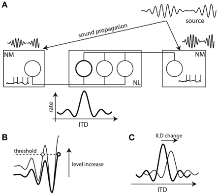
Figure 1. ITD processing in the barn owl and the level invariance problem. (A) ITD processing in the barn owl. The sound arrives earlier at the closer ear and with louder intensity. It is encoded into spike trains by monaural neurons in the Nucleus Magnocellularis (after peripheral auditory processing, not shown). These neurons project axons to binaural neurons in the Nucleus Laminaris with various conduction delays. When the interaural time delay (ITD) matches the difference in conduction delay, the neuron receives synchronous inputs and fires (emphasized neuron). As a result, neurons are tuned to a particular ITD called the “best delay.” (B) When the input level is increased, integrating to a fixed threshold in NM neurons implies that spikes are produced earlier. (C) If level is changed at one ear, meaning a change in interaural level difference (ILD), the tuning of binaural neurons should be shifted.

One remarkable feature is that the ITD tuning of binaural neurons persists when the acoustic level is varied over as much as 70 dB (Peña et al., 1996), that is, the best delay does not depend on level. It is also hardly affected by ILD (Takahashi et al., 1984). In terms of acoustic pressure, 70 dB corresponds to a scaling by a factor greater than 3000. The challenge for the neural circuit which implements this operation is illustrated in Figure 1B. Assuming that monaural neurons fire when their input reaches a fixed threshold, they tend to fire earlier when the level increases. If the levels are different in the two ears (i.e., if the ILD is non-zero), these changes in timing could be different in the two monaural neurons, resulting in a change in preferred interaural delay of the binaural neuron (Figure 1C).

How can a monaural neuron encode sounds in a way that preserves timing? There are essentially two possible scenarios (considering only single-cell mechanisms):

1. The neuron is very noisy, so that its response to small signals is approximately linear (Fourcaud and Brunel, 2002). In this case, phase information is preserved and the response of the binaural neuron approximates the cross-correlation of the two monaural signals. However, this poses at least two problems. First, it implies that the firing rate increases linearly with level, but the firing rate cannot increase 3000-fold. Second, the resulting tuning curve for interaural delay is only mildly selective.

2. The neuron is not noisy, and a gain control mechanism exists that insures that spike timing and firing rate do not depend on level.

It seems that the second scenario is closer to the known properties of NM neurons. Indeed, their firing rate saturates very quickly (Fukui et al., 2010) while still providing accurate timing information to the binaural neurons in NL (Peña et al., 1996). In addition, these neurons fire at precise phases of pure tones at high frequencies (Koppl, 1997). In the cat, bushy cells in the cochlear nucleus (analogs of NM neurons in birds) respond to frozen noises with submillisecond precision, indicating a very low level of intrinsic noise (Louage et al., 2005). ITD selectivity properties of binaural neurons in the cat inferior colliculus are also remarkably insensitive to level (Yin et al., 1986).

Part of this phenomenon can be accounted for by the active mechanics of the basilar membrane, prior to the initiation of any spike in the auditory periphery (Robles and Ruggero, 2001), and by the saturation of auditory nerve fibers. I will come back to this issue in the discussion, but at this point I simply note that NM neurons are less sensitive to level than AN fibers, as is shown in Figure 2.

FIGURE 2

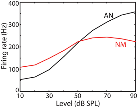
Figure 2. Average firing rate as a function of input level in auditory nerve (AN) fibers and NM neurons of the chicken (replotted from Fukui et al., 2010).

These observations motivate the central question of the present study: how can the responses of a neuron be insensitive to input level, and what cellular mechanisms does it imply? First, I will describe the constraints that level invariance imposes on spiking models, independently of biological constraints. Then, taking physiological constraints into account, I will describe the implications of level invariance in terms of ionic channel properties.

2. Theoretical Spiking Models

In this section, I derive necessary conditions for a spiking model to produce spike trains in a way that does not depend on input level. This means that both the timing and rate of output spikes are insensitive to level – possibly after a transient convergence phase.

Consider a spiking neuron, which fires when its membrane potential reaches a threshold (Figure 3). We require that the spike trains remain unchanged when the input level is varied and we derive necessary conditions. Let us focus on one interspike interval. When the input level is varied, the membrane potential changes. To preserve the timing of the spike, the scaling of the input should leave the crossing point unchanged (open circles in Figure 3), and not produce new ones: this implies that the threshold cannot be fixed. Thus, the spike threshold must somehow follow changes in membrane potential.

FIGURE 3

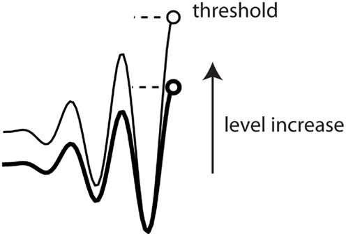
Figure 3. Threshold in a level-invariant spiking model: when the membrane potential is increased (the two curves), the threshold (dashed lines) must increase in the same proportion to keep spike timing unchanged.

2.1. A Simple Model

We start with a simple model that exhibits level invariance (Figure 4). A spike is produced when the input I(t) reaches a dynamic threshold θ(t) – there is no membrane equation for the moment. When the input is scaled: I → λI, the threshold must scale in the same way: θ → λθ. This occurs if the threshold depends linearly on the input. In terms of dynamical systems, this means that θ is governed by a linear differential equation (or set of equations), for example:

FIGURE 4

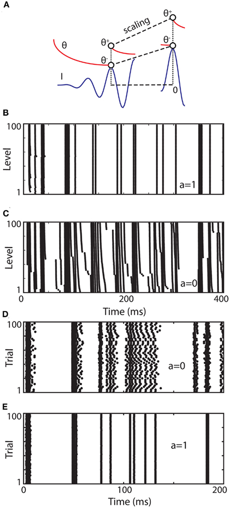
Figure 4. A simple level-invariant spiking model. (A) A trajectory of the model is scaled (blue: input I, red: threshold θ): the ratio θ⁺/θ⁻ is constant. (B) Responses of a level-invariant model (τ_θdθ/dt = I − θ, θ → 2θ at spike time) to a fluctuating input with level varying between 1 and 100. (C) Same as in (B), but with the special case τ_θdθ/dt = − θ. (D) Same as in (C), but level is identical in all trials while initial condition is different (random between 0 and 1). (E) Same as in (D), but with the model shown in (B).

where a is a fixed parameter. Note that the equilibrium value for the threshold must be 0 in the absence of input.

After a spike, the threshold must increase, from θ⁻ = θ(t⁻) to θ⁺ = θ(t⁺), so that the spiking condition is not met anymore. For simplicity, let us assume that θ⁺ only depends on θ⁻: θ⁺ = f (θ⁻). How precisely the threshold increases can now be derived from the assumption of level invariance. Suppose that we scale the input, and therefore the trajectory θ(·) so that crossing points are unchanged (Figure 4A): I → λI and θ(·) → λθ(·). Both θ⁻ and θ⁺ are scaled in the same proportion, so that the ratio θ⁺/θ⁻ is constant. We denote this ratio ρ and we obtain the following reset condition at spike time: θ → ρθ. We note that ρ > 1, since the spiking condition must not be met after the spike.

These considerations have led us to the following elementary level-invariant spiking model:

where ρ and τ_θ are two free parameters. We note that the initial condition for θ must be positive (assuming the input is initially zero). Figure 4B illustrates the level invariance property of this model with a = 1 and τ_θ = 10 ms, which was driven by a fluctuating input with level varying by a factor 100. This input I(t) was defined by the following stochastic differential equations:

where ξ(t) is Gaussian white noise, and τ = τ_θ = 10 ms. The initial condition was identical in all runs (θ = 1). All models in this paper were simulated with the Brian simulator (Goodman and Brette, 2009).

In Figure 4C, the same simulations were done with a = 0, and it appears that responses are not identical in all trials (where level varies from 1 to 100, as in Figure 4B). This is surprising because the model satisfies the same properties as in Figure 4B and should be level-invariant. The reason is that for a = 0, responses to the same input (same level) are also not reproducible across trials, if initial conditions are different (as in Figure 4D) or if there is some intrinsic noise. In contrast, responses to the same input are reproducible across trials with a = 1 when the initial condition differs (Figure 4E), after a transient synchronization time. In general, spike trains produced by spiking models in response to time-varying inputs are robust to changes in initial conditions and stochastic perturbations (Brette and Guigon, 2003; Brette, 2004, 2008), but there are special cases where the dynamics is unstable, as in Figure 4D. To understand why, consider the perfect integrator, which is an example of such a special case:

The neuron fires when X = 1 and is then reset to 0. If two solutions X₁ and X₂ start with different initial conditions X₁(0) ≠ X₂(0), then the difference X₂(t) − X₁(t) never changes (modulo 1) and therefore the solutions never converge: spike timing is not reproducible. From a dynamical point of view, spiking in this model is equivalent to a temporal translation t → t + 1/〈I〉 (where 〈I〉 is the average input). A similar phenomenon occurs in the level-invariant model with a = 0, that is, it can be shown that spiking in this model is topologically equivalent to a temporal translation t → t + τ_θ log ρ, which implies that the model is sensitive to initial conditions and stochastic perturbations (see the proof in Appendix B). What happens in this case when the level is changed: I → λI? Our mathematical considerations imply that if θ(t) is a solution for the initial level, then the scaled trajectory λθ(t) will be a solution for the scaled level, with spikes occurring at the same times. That is, the solution starting from initial condition λθ(0) will spike at the same times. However, the solution with initial condition θ(0) will not fire at the same times with the scaled level, because of the dynamical instability of the model. However, the firing rate is level-invariant [equal to (τ_θ log ρ)⁻¹], as well as the set of possible solutions (for all initial conditions). Thus, Figure 4C does not show a lack of level invariance, but a lack of reproducibility of the model responses for a = 0. In contrast, in Figure 4B, the model responds at the same times for all levels, but only after a transient synchronization time. This is because the model always starts with the same initial condition, rather than with scaled initial conditions (λθ(0)), and this synchronization time reflects the time required for solutions with different initial conditions to converge, as shown in Figure 4E.

The firing rate (which is also level-invariant) can be calculated for a constant current I = 1 (remember that it does not depend on the value of that current). Consider one interspike interval (0, T). The threshold is θ(0) = ρ at the beginning and at the end. Since a spike is produced at time T, we have θ(T) = I = 1 and therefore:

provided this is well defined. The firing rate is the inverse of this quantity. Note that the firing rate does not depend on level, but it may depend on other aspects of the time-varying input. The value we have calculated is only valid for constant inputs.

One important point has been neglected: if the input I is allowed to be negative, then the threshold θ may become negative as well. If a spike is produced when θ < 0, the reset θ → ρθ pushes the threshold below the input, which produces an infinite sequence of spikes. There are two simple ways to deal with this problem: (1) to replace I by the half-wave rectified input [I]⁺ = max(0, I); (2) to consider a different reset when θ < 0: θ → γθ, with γ < 1. In fact, we must have γ < 0 to avoid infinite sequences of spikes (e.g., θ → −θ). It can be seen that the model is still level-invariant with these modifications.

As an example, Figure 5 shows how level-invariant models encode vowels. Figures 5A,B shows the responses of a noisy level-invariant model to the vowel I, band-pass filtered around 1 kHz. The noise was modeled as follows: input I is replaced by I(1 + n), where n is an Ornstein-Uhlenbeck process with time constant 5 ms and SD 0.03. The same vowel was presented 100 times to the model, and the spike trains of all trials are shown (each dot represents a spike). The figure shows that spike timing is precise and can thus be used as a reliable temporal cue for source localization. In Figures 5C,D, a vowel (I in Figure 5C and A in Figure 5D) is presented a single time, but to 1000 neurons with different central frequencies, representing basilar membrane filtering. That is, the vowel is passed through a bank of band-pass filters (gammatone filters), with frequencies between 20 Hz and 20 kHz (with regular ERB spacing), half-wave rectified and compressed (1/3 power law), and the filter outputs are the inputs of the models. This filtering is implemented using Brian Hears, an auditory toolbox for the Brian simulator (as in Figure 1 in Fontaine et al., 2011).

FIGURE 5

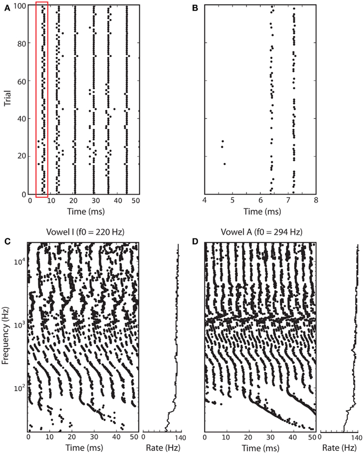
Figure 5. Responses of level-invariant models to vowels. Two vowels were filtered through 1000 gammatone filters with frequencies between 20 Hz and 20 kHz (with regular ERB spacing), half-wave rectified and compressed (1/3 power law). The processed signals were inputs to noisy level-invariant spiking models (τ_θdθ/dt = I − θ, θ → 3θ at spike time, τ_θ = 5 ms; noise is added to the input I, independently for all neurons). (A) Responses of the neuron with preferred frequency 1 kHz to 100 repeated presentations of vowel I (each dot is a spike). (B) Zoom of the red box in (A). (C) Responses to vowel I at fundamental frequency f0 = 220 Hz (A3), and firing rates of all neurons (right). (D) Responses to vowel A at fundamental frequency f0 = 294 Hz (D4).

Here, we note that the pitch (periodicity of the sound) appears in the periodicity of the spiking pattern (notice the smaller period in B). Note that spiking patterns may repeat at a higher rate than the firing rate (220 vs. 140 Hz in A) because firing is stochastic (neurons do not fire on every period). Finally, firing rate is insensitive to level but not to other aspects of the input, such as spectral content: for example, lower frequency neurons fire at a lower rate.

I now consider increasingly complex models, in an attempt to characterize a large class of spiking models that exhibit level invariance.

2.2. Linear Spiking Models

In physiological neuron models, the input is not directly compared to the threshold. Instead, the input changes the membrane potential v through a differential equation named the “membrane equation,” and that potential is compared to the threshold. The same analysis as before applies if the input I is replaced by v, and the membrane potential scales linearly with level. This is the case if the spiking model is described by a linear differential system, for example (but not limited to):

where v is the membrane potential, τ is the membrane time constant, and R is the membrane resistance. Note that the resting potential is defined as 0. The differential system may be non-autonomous, that is, its coefficients may depend on time (but not on voltage). Equivalently, the membrane potential can be described by the linear convolution of the input with a (possibly time-dependent) kernel K: v = K * I, as in the Spike Response Model (Gerstner and Kistler, 2002). The analysis below is unchanged if the membrane potential scales linearly with a function of level f(λ), since it simply amounts to replacing the scaling parameter λ by f (λ) – this remark will become important in section 3.

As in the previous section, the threshold should depend linearly on the membrane potential in order to keep crossing points unchanged when the level changes. Thus, the dynamic threshold can be described by a linear differential system or, equivalently, as the linear convolution of the membrane potential with some filter K_θ: θ = K_θ * v. The simplest such system consists of one differential equation: τ_θ(dθ/dt) = av − θ. One deviation from linearity can be allowed: since we consider linear scaling with positive numbers only, the model can include half-wave rectification:

where [v]⁺ = max(0,v). More generally, the threshold may be governed by a different linear differential system for v > 0 and v < 0. Even more generally, the system may be piecewise linear, each piece being defined by the condition K_i * v > 0, where K_i is a linear filter. The same remark applies to the membrane equation.

Finally, the threshold can also be described as a sum of variables θ = θ₁ + θ₂, where θ₁ and θ₂ are governed by equations as above. This allows different timescales in threshold dynamics.

2.3. Threshold, Reset, and Refractory Period

At spike time, we have shown in section 1 that the threshold must change by a constant multiplicative factor: θ → ρθ. To derive this condition, we assumed that the threshold only depended on the value of the threshold at spike time. If the threshold is a sum of components (θ = θ₁ + θ₂), then each component may be reset independently: θ₁ → ρ₁θ₁ and θ₂ → ρ₂θ₂. More generally, any reset preserves level invariance if it scales linearly with membrane potential. In particular, it may depend on a hidden variable u: θ → ρθ + γu, where u depends linearly on the membrane potential (e.g., through a linear differential system).

The same analysis applies to the reset of the membrane potential. If it only depends on the value of v at spike time, then it must also be multiplicative: v → γv. Two simple cases are a fixed reset to the resting potential: v → 0, and no reset at all. To keep the analysis simple, we now focus on the simplest cases θ → ρθ and v → γv.

To ensure that the membrane potential is below threshold after a spike, the following condition must be met: (ρ − γ)θ⁻ > 0 (remember that θ⁻ = v⁻). As we previously noted, this implies that either ρ > γ and the dynamic threshold is always positive (if the input is positive or if the threshold depends on the half-wave rectified version of the membrane potential), or ρ − γ must also change sign for negative potentials. For positive potentials, the reset parameters must satisfy the following inequality: ρ > γ, and if negative thresholds are possible, then we must have ρ < 0 and ρ < γ for negative potentials.

However, in practice, the condition ρ > γ is not sufficient. Consider for example the case ρ = 1, γ = 0, and a = 0, that is, no reset for the threshold and fixed reset for the membrane potential, and the threshold does not adapt:

In this case, the dynamic threshold converges exponentially to zero, which means that the neuron spikes at an exponentially increasing rate (Figure 6). Thus, even though the model is level-invariant, it is not of any practical use. How can this situation be avoided? Suppose that at some point the threshold is hit at a very small value δv, then it is reset to ρδv. The threshold is then hit again after a small time δt, of magnitude δv (this follows from the equality δv + δt × dθ/dt = ρδv + δt × dv/dt). The derivative of the threshold is proportional to δv, so that the increase in threshold after that time has magnitude (δv)², that is, it does not significantly change during the interspike interval and remains about ρδv (at first order in δv). After n spikes, the spike threshold is then ρⁿδv. Thus, if ρ < 1, the threshold converges exponentially fast to zero (and an infinite number of spikes are produced in finite time); if ρ > 1, then the threshold is repelled from zero at an exponential rate. If ρ = 1, a simple calculation shows that the threshold is repelled if aγ > 1, but at a slow rate. In summary, in addition to the condition ρ > γ, we must have ρ > 1 or ρ = 1 and aγ > 1 to avoid infinite spiking, and ρ > 1 to avoid strong bursting.

FIGURE 6

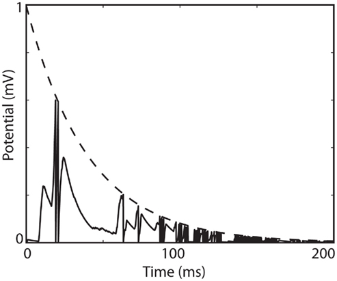
Figure 6. Infinite firing in a level-invariant model with a fluctuating input (Ornstein-Uhlenbeck process with time constant 3 ms; model parameters were τ = 10 ms and τ_θ = 40 ms). The dynamic threshold (dashed) is non-adaptive (a = 0) and is not reset at spike time (ρ = 1). The membrane potential (solid line) is reset at spike time (v → 0).

An absolute refractory period can be included in two ways: (1) by considering that I = 0 for a duration Δ after the spike, (2) by clamping the membrane potential at reset for a duration Δ. Both options are compatible with level invariance, because the values of the threshold and membrane potential at the end of the refractory period scale linearly with their values at reset time, and therefore with level.

Relative refractory periods can be included with spike-triggered currents, which we examine in the next section.

2.4. Spike-Triggered Conductances

In general, inserting spike-triggered currents in the membrane equation breaks level invariance, because they do not scale with level. However, the situation is different if we consider spike-triggered conductances, that is, the current is modeled as I_s(t) = g(t)(E − v), where the conductance g(t) is determined by the spike trains only (not by the membrane potential) and E is the reversal potential. Since the membrane potential scales with level, such a current also scales with level if E = 0 (reversal potential equals resting potential). Note that the dynamics of the conductance g(t) can be arbitrarily complex, as long as it only depends on the spike trains.

For example, the following model is level-invariant:

and g → g + Δg at spike time (we assume that threshold and reset are described as before). Note that this model cannot be described by a linear time-invariant filter anymore (the effective time constant τ/(1 + g) is now dynamic), but it is still level-invariant.

To end this part, Figure 7 shows an example of a complex level-invariant model, which includes several of the components we have discussed (the fluctuating input was generated as in Figure 4).

FIGURE 7

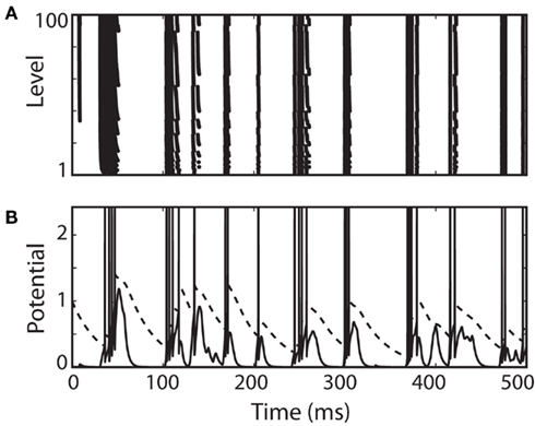
Figure 7. A complex level-invariant spiking model with a membrane equation and an adaptive threshold, multiplicative reset of threshold and membrane potential, and spike-triggered conductances. (A) Responses of the model to a fluctuating input (low-pass filtered Ornstein-Uhlenbeck process with time constant 4 ms, as in Figure 4) with level varying between 1 and 100. (B) Trace of the membrane potential (solid) and dynamic threshold (dashed) for the lowest level. Spikes were drawn for clarity.

3. Physiological Implementation

In deriving the implications of level invariance on spiking models, we have not considered physiological constraints yet. There are mainly two issues to consider. First, the constraints on threshold dynamics imply very specific ionic channel properties. Second, the dynamic range of the membrane potential is limited (since it is bounded by the reversal potentials of the various ionic channels), and specific mechanisms are required to deal with this issue.

3.1. The Dynamic Threshold

In this section, I will only consider transient sodium currents responsible for spike initiation. Other sodium currents are persistent or slowly inactivating, and activate at low voltages. In this case they may produce subthreshold oscillations, which would presumably disrupt the level invariance mechanism we are interested in, in particular because the frequency of these oscillations depends on depolarization (Gutfreund et al., 1995).

3.1.1. Voltage adaptation

The key property for level invariance is that the threshold adapts to the membrane potential. This phenomenon can indeed occur in neurons because Na channels partially inactivate when the neuron is depolarized (see for example Howard and Rubel, 2010 for threshold dynamics in NM neurons of the chick). In neuron models with Hodgkin-Huxley sodium current dynamics, it can be shown that the dynamic threshold depends on the proportion of non-inactivated channels h through the following threshold equation (Platkiewicz and Brette, 2010):

where V_T is the minimum threshold and k_a is the activation slope factor of Na channels (typically, k_a ≈ 6 mV; Angelino and Brenner, 2007). From the dynamics of h, a differential equation for the threshold can be derived (Platkiewicz and Brette, 2011):

where τ_θ(v) is the inactivation time constant and θ_∞(v) = V_T − k_a log h_∞(v) is the steady-state threshold (this differential equation is an approximation, which is valid when θ is near θ_∞(v)). Inactivation curves h_∞(v) are well approximated by Boltzmann functions:

where k_i is the inactivation Boltzmann factor and V_i is the half-inactivation voltage. Because of this specific form, it can be seen that the steady-state threshold is well approximated by a rectified linear function (Platkiewicz and Brette, 2011):

The quality of this approximation depends on the sharpness of the inactivation curve, which is controlled by k_i: it becomes exact in the limit k_i → 0. Thus, the dynamic threshold equation is consistent with the constraints we have derived for level invariance if all the following conditions are met:

1. V_T = 0 and V_i = 0 (where the resting potential is taken as the reference potential, i.e., E_L = 0 mV as in section 2; otherwise the equality is V_T = V_i = E_L). This means that the minimum threshold V_T, which is controlled by the maximum Na conductance (Platkiewicz and Brette, 2010), is at the resting potential, and therefore the neuron spontaneously fires to an arbitrarily small level of intrinsic noise. This is not consistent with slice experiments (Reyes et al., 1994), but it is consistent with in vivo data, showing that spontaneous rates of NM neurons are very high (Warchol and Dallos, 1990; Köppl, 1997) – see also (Kuenzel et al., 2011) for recent in vivo data in spherical bushy cells of the gerbil. The half-inactivation voltage V_i must also be near resting potential, which means that half Na channels are inactivated at rest. This is consistent with typical values found in voltage-clamp recordings (Howard and Rubel, 2010; Platkiewicz and Brette, 2011).

2. τ_θ(v) is constant. This is an approximation that is only valid in a limited voltage range.

4. k_i is small. Typical values are in the range 4–8 mV (Angelino and Brenner, 2007), which is not so small. This means that the transition between the two linear parts of the steady-state threshold curve is not so sharp.

Problem 3 can be solved if inputs are positive (that is, only excitatory), by choosing a negative V_i, and V_T = (k_a/k_i)V_i < 0. Indeed in this case, θ_∞(v) = (k_a/k_i)v for all positive v. It is negative for negative v, but this never occurs for positive inputs. Precisely, the dynamic threshold equation reads:

where the right hand side is formally equivalent to (k_a/k_i)[v]⁺ − θ for positive voltages. If V_i is hyperpolarized enough, then we have v − V_i ≫ k_i (since v is always positive) and the membrane potential always lies in the linear range of the steady-state threshold curve. The condition V_T = (k_a/k_i)V_i < 0 assumes E_L = 0 mV (the resting potential is the reference), otherwise it reads: V_i < E_L and V_T = E_L + (k_a/k_i)(V_i − E_L).

Another issue is the sharpness of spike initiation. In the previous section, we assumed that spike initiation is sharp, that is, a spike is produced as soon as voltage threshold is reached, as in an integrate-and-fire model. Physiologically, this means that no Na current flows below threshold, and that a very strong current flows as soon as threshold is reached. This is not necessarily so in a real neuron or a Hodgkin-Huxley model. A more rigorous way to describe threshold modulation (e.g., by Na inactivation) is to see it as a shift in the excitability curve of the neuron, rather than as a shift of the voltage threshold per se, because the voltage threshold is generally not a well defined quantity with fluctuating inputs (at least in single-compartment Hodgkin-Huxley models). More precisely, the Na current can be approximated by an exponential function (Fourcaud-Trocme et al., 2003; Badel et al., 2008): I_Na = k_ag_Lexp((v − V_T)/k_a), which becomes I_Na = k_ag_L exp((v − V_T + k_a log h)/k_a) when inactivation is considered (Platkiewicz and Brette, 2010). Thus, even though there is no sharp threshold, the current-voltage curve of the neuron is voltage-shifted by inactivation according to the threshold equation. However, this current is not level-invariant because k_a does not scale with level. Therefore, it seems desirable that spike initiation be as sharp as possible. There are two possibilities to obtain this property:

1. k_a is small. But typical estimates from voltage-clamp studies are in the range 4–8 mV. However, these have been obtained by fitting Boltzmann functions on the entire voltage range and may not be accurate estimates near spike initiation (Fourcaud-Trocme et al., 2003; Platkiewicz and Brette, 2010).

2. Spike initiation is made sharper by axonal backpropagation. This is a subtle issue that has been revived a few years ago, after a controversy on the validity of the Hodgkin-Huxley model for cortical neurons (Naundorf et al., 2006; McCormick et al., 2007). In cortical neurons, spikes are initiated in the axon hillock, about 35–50 μm away from the soma (Palmer and Stuart, 2006; Shu et al., 2007), and actively backpropagated to the soma (Yu et al., 2008). This makes spikes sharper than they would be if there were a single electrotonic compartment (this can be seen in the cable equation, because the diffusion term is positive at spike initiation). Indeed, measurements in cortical neurons yield estimates of sharpness around 1 mV rather than k_a ≈ 6 mV (Badel et al., 2008; Rossant et al., 2010). It should be noted that when distal initiation is considered, threshold modulation is still proportional to k_a, but this quantity is no longer directly related to the sharpness of spike initiation (Platkiewicz and Brette, 2010). However, to my knowledge, sharpness of spike initiation has not been studied in subcortical areas such as the auditory brainstem.

3.1.2. Reset

In a model with Hodgkin-Huxley Na current dynamics, the threshold also increases after each spike, because Na channels inactivate during the action potential. We showed that this modification must be multiplicative to preserve level invariance, but simple considerations suggest that spike-triggered modifications of the threshold should be additive (Platkiewicz and Brette, 2010): θ → θ + ρ. This comes from the approximation that h_∞(v) = 0 during the spike, which implies that h(t + Δ) = h(t)exp(− Δ/τ_h), where t is the time of spike initiation and Δ the spike duration. It follows that the threshold is shifted by a constant term: θ → θ + k_aΔ/τ_h.

Although this is a crude approximation, the result is more general, if spike shape is not significantly affected by threshold modulation. The dynamics of h is governed by the following differential equation:

and if the spike shape is fixed, that is, v(t) is fixed, then this is a non-autonomous linear differential equation. Therefore, h(t + Δ) depends linearly on the initial condition h(t): h(t + Δ) = λh(t) (for some value λ which is determined by the spike shape and inactivation properties). Again, this implies an additive shift of the threshold.

In pyramidal cortical neurons, spike shape is not always very variable, possibly because of axonal backpropagation and the presence of other Na channel types with higher activation and inactivation voltages (Hu et al., 2009). However, this is not the case of all neurons (e.g., interneurons). When the threshold is higher, spike peaks tend to be lower because of the decreased availability of Na channels (de Polavieja et al., 2005). This should make threshold shifts inversely correlated with threshold (the opposite of what is needed), but this effect should be small: if the peak exceeds threshold by more than a few times k_i (that is, by about 10 mV), then the steady-state inactivation h_∞(v) is effectively zero during the spike. Thus, the main determinant of the threshold shift should be spike width (about k_aΔ/τ_h). Therefore, to obtain multiplicative threshold shifts after each spike, spike width should be proportional to spike threshold. There is some experimental evidence that spike width is indeed positively correlated with spike threshold in pyramidal cells: in (de Polavieja et al., 2005), spike height was found to be negatively correlated with spike width, and spike height is also negatively correlated with spike threshold.

Spike width is essentially controlled by the potassium rectifier current (Carter and Bean, 2009): indeed the speed of repolarization is roughly proportional to the total conductance of the rectifier channel, therefore spike width is inversely proportional to that conductance. Thus, multiplicative threshold modulation requires that the conductance of these channels is inversely proportional to spike threshold, that is, with the value of the membrane potential at spike initiation. We may think of two mechanisms: (1) with higher threshold values, spike height is reduced and therefore potassium channels activation is reduced, meaning wider spikes, (2) potassium channels may inactivate, so that higher threshold values imply more inactivated potassium channels and therefore wider spikes. This second mechanism is only possible if rectifier channels inactivate with fast dynamics. If the inactivation curve is a Boltzmann function, then the inverse of the inactivation variable (proportion of available channels) is We want this quantity to scale linearly with the membrane potential v, but clearly this can only be approximately valid. large? Nevertheless, this analysis suggests that several factors may make the threshold modulation due to a spike more complex than a simple additive shift. As many factors are involved (including neuronal morphology), this relationship should be empirically measured, either in vivo or in slice with fluctuating injected currents.

Finally, note that the reset of the membrane potential is irrelevant in a biophysical model, since it is implicitly implemented by the potassium rectifier channels. As we have seen in section 2, the condition for level invariance is that the reversal potential of these channels equals the resting potential.

3.1.3. Multiple timescales

Na channels inactivate both on fast and slow timescales. A simple model consists of two independent gating variables:

where the gating variables h_slow and h_fast have slow and fast dynamics, respectively (Fleidervish et al., 1996; Kim and Rieke, 2003). Since the interaction is multiplicative for the Na current, it is additive for the threshold:

and both components of the threshold are described as previously.

3.2. The Dynamic Range Problem

In section 2, we have assumed that the membrane potential scales linearly with level. This is problematic because physiologically, the membrane potential must be bounded by the minimum and maximum reversal potentials. In practice, the dynamic range for the membrane potential does not exceed a few tens of millivolts. If the dynamic range of the input is very large, then some compression is necessary. Suppose the input level can change by a factor 100 but the voltage range is only allowed to change by a factor 10 (say, the amplitude of voltage fluctuations can vary between 2 and 20 mV). Then between the two extreme levels, the membrane resistance must change by a factor 100/10 = 10. In other words, the dynamic range for the membrane resistance equals the ratio of dynamic ranges of the level and membrane potential. This implies the presence of a very strong conductance with a steeply increasing activation curve. Assuming that the activation curve is a Boltzmann function, this means that the half-activation voltage is high, so that it approximates an exponential function in the subthreshold regime. We consider a slow voltage-activated conductance with reversal potential E, for example a potassium channel. Since it is slow, the conductance only depends on the average membrane potential 〈v〉, so that the membrane equation reads:

with an approximately exponential conductance:

This implies that the average membrane potential is an approximately logarithmic function of level. The membrane equation can be rewritten as follows:

where g depends on 〈v〉. One issue is that the effective membrane time constant depends on the conductance g, and therefore on level. For example, for sinusoidal inputs it implies level-dependent phase shifts. The problem is solved if the membrane time constant is small compared to the input frequency range: τ ≪ 1/(2πf ), so that the phase is preserved. This is a serious constraint for high-frequency inputs. The alternative is that the minimum membrane time constant is large compared to the input frequency range: τ/g_max ≫ 1/(2πf ). In this case, the phase is not preserved but is insensitive to level (cosine phase). If the time constant issue is solved, the membrane potential scales linearly with a function of level, provided E = 0, so that the level invariance constraints are still satisfied.

Figure 8 shows the same complex spiking model as in Figure 7, but with an additional strong K high-voltage-activated conductance. The level invariance property is now only approximately satisfied (Figure 8A), but considering that the level changes by a factor 100, the performance is reasonable. Because of the strong intrinsic conductance, the average membrane potential does not increase proportionally to the level, and some compression appears (Figure 8B). As a result, the membrane potential remains within a physiologically reasonable range, even at high input levels (Figure 8C). To accomplish this compression, the K conductance increases by a factor 7 when the level increases by a factor 100 (Figure 8D).

FIGURE 8

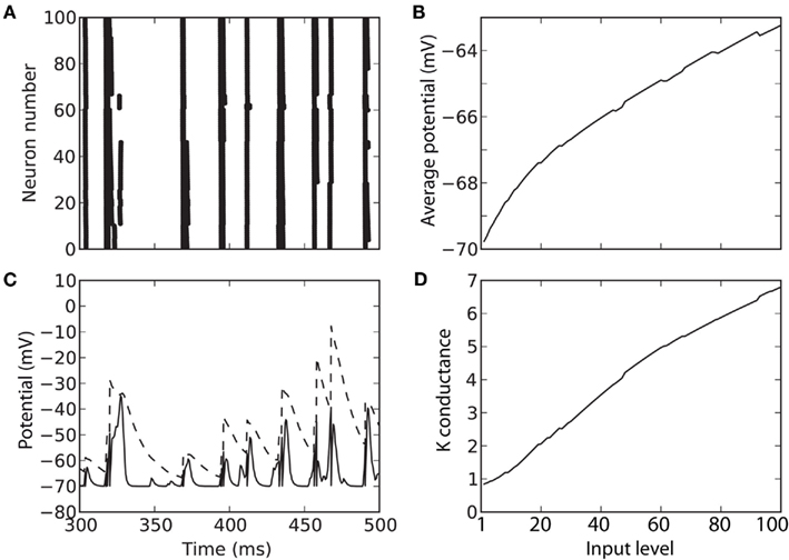
Figure 8. Response of a level-invariant model with strong K conductance. The model is similar to the model in Figure 7, but with an additional K conductance with time constant 50 ms, Boltzmann activation (V_a = − 50 mV and k_a = 5 mV) and maximal conductance equal to 50 times the leak conductance. (A) Responses of the model to a fluctuating input (low-pass filtered Ornstein-Uhlenbeck process with time constant 2 ms), with level varying between 1 and 100. (B) Average membrane potential as a function of input level. (C) Trace of the membrane potential (solid) and dynamic threshold (dashed) for an intermediate level (50). Spikes occur at the crossing points. (D) Average K conductance as a function of input level, relative to the leak conductance.

3.3. The Dynamic Threshold Again

In section 1, we considered the effect of Na inactivation of threshold dynamics. However, the threshold also varies with the total conductance (in particular K+ conductance) in the following way (Platkiewicz and Brette, 2010):

Thus, strong conductances as discussed in the previous section should have a strong impact on the threshold. As we considered channels with high activation voltage and strong maximal conductance , the conductance is

Therefore the shift in voltage due to this conductance is

Thus the threshold reads:

where

Since the last term in the threshold formula scales linearly with the membrane potential, the previous discussion applies when V_T is replaced by That is, the threshold still scales with membrane potential if

4. Discussion

4.1. Summary

In many sensory modalities, the stimuli that neurons must encode vary in intensity over several orders of magnitude. Thus, efficient encoding requires some form of gain control. Indeed neuromorphic sensors, such as spiking electronic retinas (Posch et al., 2008) and cochleas (Liu et al., 2010), all address this problem. For example, in the DVS electronic retina (Posch et al., 2008), a spike is produced when pixel intensity changes by a fixed logarithmic increment. In the sound localization system, this is a very critical issue because precise estimation of the interaural time difference (a major cue to azimuth) relies on the comparison of spike timings at a microsecond scale. In a standard integrate-and-fire model, the neuron tends to fire earlier when stimulus intensity increases. To avoid this problem requires that the spike threshold changes with stimulus level. The simplest level-invariant spiking model is the following:

where ρ > 1 and a > 0 (I is the time-varying level, θ is the threshold). Its firing rate is T = τ_θ log((ρ − a)/(1 − a)) for constant inputs. More generally, we have seen that a fairly large class of (phenomenological) spiking neuron models exhibits level invariance, which is described by the following conditions:

• The membrane potential changes linearly with level, or with a function of it. This occurs for example if it is governed by a linear differential system, where the input I (or RI, where R is the membrane resistance) is added to one differential equation (typically the membrane equation).

• The threshold is dynamic and depends linearly on the half-wave rectified membrane potential [v]⁺, or on the membrane potential v if I > 0. This occurs for example if it is governed by a linear differential system, where the membrane potential v (or av) is added to one differential equation. The threshold may be described as a sum of components θ = θ₁ + θ₂ with different dynamics.

• After a spike, both the threshold and membrane potential are multiplicatively reset: θ → ρθ and v → γv, with ρ > 1 and ρ > γ (ρ = 1 is possible, provided that aγ > 1).

• After a spike, an absolute refractory period of duration Δ may be considered, by either ignoring the input (I = 0) or clamping the neuron at reset.

• Spike-triggered conductances with arbitrary dynamics may be included, provided that the reversal potential equals the resting potential, i.e., the current is I(t) = − g(t)v.

These conditions imply some specific constraints on ionic channel properties, which translate to the following constraints:

• Spike initiation is sharp.

• Na channels half-inactivation voltage V_i ≤ 0 (where 0 is the resting potential) and This value takes into account the properties of Na channels and K rectifier channels (more generally, high-voltage-activated conductances). This second condition essentially means that the spike threshold equals the resting potential.

• Inactivation slope k_i is small.

• Spike width is positively correlated with spike threshold.

• There is a strong hyperpolarizing conductance with high half-activation voltage and slow dynamics (rectifier conductance).

• The reversal potential of rectifier channels equals the resting potential.

• There are no significant subthreshold oscillations – which could be due for example to low-voltage-activated persistent sodium (Gutfreund et al., 1995).

Figure 9 shows how level-invariant spiking models can be used in the context of ITD processing. A binaural neuron, modeled as a standard noisy integrate-and-fire neuron, receives inputs from 40 monaural neurons on each side, which are driven by band-pass filtered noise with varying ITD and ILD. When monaural neurons are modeled as standard integrate-and-fire neurons (Figures 9A,B), neurons on the louder side fire more and earlier (Figure 9A), and as a result, the best delay of the binaural neuron depends on ILD (Figure 9B). When monaural neurons are modeled as level-invariant spiking models, this ILD-dependent bias does not occur (Figures 9C,D). Note that the tuning curves for non-zero ILDs in Figure 9D are above the tuning curve for zero ILD because neurons on the louder side initially fire more spikes (and ILDs were introduced by raising the level of either side).

FIGURE 9

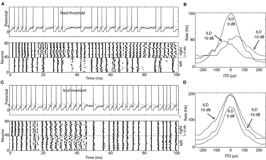
Figure 9. ITD tuning curve of binaural neuron model, with monaural neurons modeled as either integrate-and-fire neurons (A,B) or level-invariant models (C,D). (A) A binaural white noise input is passed through a of gammatone filter centered at 2 kHz, compressed (1/3 power law) and half-wave rectified. The filtered input is fed into 80 monaural (NM) neurons, 40 on each side, modeled as noisy integrate-and-fire neurons (time constant 1 ms, refractory period 1 ms, noise SD 0.03, voltage is in units of the threshold). Top: membrane potential of one NM neuron (dashed line: threshold). Bottom: spike trains produced by all 80 neurons, with 0 ms ITD and 10 dB ILD, i.e., the input sound is 10 dB louder on the right than on the left. (B) A binaural (NL) neuron is also modeled as a noisy integrate-and-fire model (time constant 0.1 ms, noise SD 0.1), and all 80 NM neurons project to the NL neuron with no delay. Each synaptic weight is w = 0.19 (instantaneous excitatory currents). The plot shows the ITD tuning curve (firing rate vs. ITD) for three different ILDs (calculated for a 5 s white noise). Thus, the best delay depends on the ILD. (C) NM neurons are now modeled as level-invariant spiking models, by simply replacing the fixed threshold by an adaptive threshold: τ_θdθ/dt = θ − v, with τ_θ = 5 ms and θ → 1.5θ at spike time. (D) The best delay of the binaural neuron [same model as in (B)] is now independent of ILD.

4.2. Comparison with Physiology

Level invariance imposes specific constraints on neuron properties. Do these constraints fit the physiological properties of bushy cells of the cochlear nucleus (mammals) and of neurons of the nucleus magnocellularis (birds)? A recent study describes threshold properties of chick NM neurons in vitro (Howard and Rubel, 2010). It was found that the spike threshold indeed adapts to the membrane potential. Consistently with our predictions, spike threshold increases linearly with the membrane potential. However, the threshold was found to be more than 20 mV above membrane potential, even at rest. A number of studies suggest that this could different in vivo. In particular, NM neurons have a high spontaneous rate in the barn owl (Köppl, 1997; greater than 200 Hz) and in the chick (Warchol and Dallos, 1990; about 100 Hz), which suggests that the threshold may be closer to the resting (or average) membrane potential in vivo. A recent study in spherical bushy cells of the gerbil confirms this hypothesis (Kuenzel et al., 2011). In addition, it was shown in this study that the firing rate of these neurons in response to pure tones varies very little over 20 dB SPL (about 200 Hz), and this property was related to the observation that the threshold EPSP size required to produce a postsynaptic spike increases with input level. Although this effect was attributed to synaptic inhibition, the results can also be explained a modulation of spike threshold as described in this paper (the mentioned study did not use pharmacological methods). For example, the frequency dependence of EPSP threshold agreed with the receptive field of excitatory inputs.

In (Howard and Rubel, 2010), threshold modulation was attributed to both K channels and Na inactivation. The membrane resistance indeed decreases by a factor of 4 over 20 mV, meaning that a strong voltage-gated conductance is present. According to our threshold equation (Platkiewicz and Brette, 2010), a four-fold increase in conductance produces a threshold increase around k_a log 4 ≈ 8.4 mV, assuming k_a ≈ 6 mV. This is a relatively small proportion of the observed range of threshold modulation (more than 40 mV). Patch-clamp studies indicate that the half-inactivation voltage of Na channels V_i is hyperpolarized, consistent with our prediction (Howard and Rubel, 2010; Platkiewicz and Brette, 2011). However, the inactivation Boltzmann factor k_i may not be very small (Angelino and Brenner, 2007).

Another potentially important requirement is that spike initiation be sharp. A few studies suggest that this is the case in cortical neurons (Naundorf et al., 2006; McCormick et al., 2007; Badel et al., 2008; Rossant et al., 2010), but it has not been specifically addressed in the auditory brainstem. Action potentials are known to be unusually short, which suggests that spike initiation is also sharp, but this specificity is most likely due to K rectifier channels (Carter and Bean, 2009). A related question is how the shape of action potentials varies with spike threshold. To implement multiplicative threshold changes at spike time, spike width should be positively correlated with spike threshold. There is some experimental evidence in pyramidal cortical cells (de Polavieja et al., 2005), but to my knowledge, this has not been quantitatively measured in the auditory brainstem. In (Howard and Rubel, 2010), threshold changes were only measured in response to presynaptic rather than postsynaptic spikes.

4.3. Peripheral Mechanisms

Although I focused on the physiology of NM neurons (and bushy cells in mammals), part of the problem can be accounted for by the active mechanics of the basilar membrane, prior to the initiation of any spike in the auditory periphery (Robles and Ruggero, 2001). In most species, active cochlear mechanics compresses the sound according to a power law with exponent around 1/3 for tones at characteristic frequency (i.e., the amplitude of basilar membrane displacement is about x^1/3, where x is the sound amplitude). This still leaves a large input dynamic range (note that this compression was taken into account in Figure 9). The auditory nerve also contributes to level invariance. Each inner hair cell (a non-spiking cell which transduces basilar membrane displacement into depolarization) makes synaptic contact with a number of auditory nerve (AN) fibers (Köppl, 2011) – 10–30 in mammals, just a couple of them in birds (more precisely, tall hair cells in these species). Collectively, the firing rate of AN fibers essentially follows the basilar membrane displacement, but individually, many fibers saturate (these are fibers with low spontaneous rate in mammals, but not in birds). Since AN fibers are the first spiking neurons in the auditory periphery, the level sensitivity issue also applies to these saturating types. Therefore, the discussion of the previous section could also apply to spike initiation in the auditory nerve. Unfortunately, there is less information available about spike threshold and ionic channels in AN fibers because intracellular recordings are technically very challenging. We note however that the level invariance issue is not entirely solved at this stage, because NM neurons are less sensitive to level than AN fibers, as is shown in Figure 2, and because the dynamic range of AN fibers tends to be larger with white noise than with tones (Greenwood and Goldberg, 1970).

4.4. Network Mechanisms

In this paper, I have only described single-cell mechanisms that can produce level-invariant responses, but neural circuits may also produce the desired property – although this is in principle more costly in terms of energy consumption, since it involves more synapses and more neurons (specifically, inhibitory cells).

We may think of two types of monaural mechanisms: feedback inhibition and feedforward inhibition. In the chicken, NM neurons are indeed modulated by GABAergic neurons in the superior olivary nucleus (SON), and pharmacological blocking of these inhibitory neurons increases the firing rate of NM neurons at high input level (Fukui et al., 2010). In both scenarios (feedback and feedforward), inhibition must increase with level to reduce the gain in proportion to input level, and be frequency-specific rather than global. In the feedforward scenario, inhibitory neurons receive inputs from other neurons which are sensitive to level. One simple possibility is strong shunting inhibition with slow dynamics: the membrane resistance is then inversely proportional to the inhibitory firing rate (note however that GABAergic input is depolarizing rather than shunting in NM neurons). To produce the desired property, inhibitory firing rate must then be proportional to the excitatory input level of the level-invariant neurons (for ITD processing, NM neurons or bushy cells), which may require some fine tuning. In the feedback scenario, inhibitory neurons receive inputs from the level-invariant neurons and modulate their gain through an inhibitory feedback loop: inhibitory neurons fire very strongly as soon as the firing rate of the excitatory neurons exceed the desired level. This solution may however cause instability problems.

We may think of an alternative mechanism to encode ITDs independently of ILDs: instead of ensuring that the output of monaural neurons is insensitive to input level (monaural mechanism), we ensure that the input levels of monaural neurons on both sides are identical (binaural mechanism). This could be implemented with cross-hemispheric interactions, for which there is some evidence in the SON (Fukui et al., 2010).

4.5. Synaptic Mechanisms

Finally, another possible mechanism to produce level-invariant responses is synaptic depression: when the level of the input stimulus increases, the presynaptic spike rate increases and the size of EPSPs decreases. Therefore synaptic depression counteracts the increase in rate with a decrease in EPSP size, so that the total synaptic input to the cell might remain approximately constant. Synaptic depression at the NM-NL synapses has been proposed as a mechanism for level invariance in sound localization in NL neurons (Cook et al., 2003), but they do not explain level invariance properties of NM neurons, or the ILD insensitivity of NL neurons. But synapses between auditory nerve fibers and NM neurons also show strong synaptic depression in vitro (Zhang and Trussell, 1994). To maintain a constant average input, the stationary EPSC size should be inversely proportional to the presynaptic spike rate. This did not seem to be the case in the study of (Zhang and Trussell, 1994), which used very young animals, but it could be quantitatively different at more physiological temperatures, in adult animals (Wang and Manis, 2008) or in vivo (Kuenzel et al., 2011). From a modeling point of view, in standard models of synaptic depression (Tsodyks and Markram, 1997), the relationship between ESPC amplitude and (inverse) presynaptic rate is non-linear, unless the recovery time constant τ_d is large compared to the typical interspike interval. This means that synaptic depression can only produce level-invariant inputs if its time constant is relatively long. This could be consistent with experimental findings, given that auditory nerve fibers generally fire at high rate (Wang and Manis, 2008).

4.6. Dendritic Mechanisms

Another mechanism that may contribute to reduce the sensitivity to input level is dendritic non-linearities. This was proposed in binaural neurons, which have a bipolar dendritic tree (Agmon-Snir et al., 1998) – although this is not the case in the barn owl. All synaptic inputs to each of the two dendritic processes originate from the same side (contralateral or ipsilateral) and produce a strong conductance, which clamps the dendritic potential to the synaptic reversal potential. This reduces the effect of input rate on dendritic potential, and ensures that binaural coincidence detection is not affected by input rate. Note that this mechanism assumes that the timing of input spikes (originating from NM neurons) is unaffected by level, and therefore it does not solve the problem I am addressing here.

We may imagine that a similar mechanism could apply to monaural NM neurons. However, it requires dendritic compartmentalization, while auditory nerve fibers make synaptic contacts (“end bulb of Helds”) onto the soma of NM neurons (Carr and Boudreau, 1991).

In conclusion, many experimental findings (threshold dynamics, strong intrinsic conductances) point to single-cell mechanisms that minimize the level sensitivity of monaural neurons in the ITD processing pathway of birds and mammals, along the lines I have described here. But it also seems that network mechanisms (inhibition by the SON) and synaptic depression could play an important role. While it may well be that many mechanisms contribute to the properties of these cells, one merit of this work is to propose phenomenological spiking models with level-invariant properties, which should be useful to develop functional models of ITD processing and possibly of other sensory processing problems.

Conflict of Interest Statement

The author declares that the research was conducted in the absence of any commercial or financial relationships that could be construed as a potential conflict of interest.

Acknowledgments

This work was partially supported by the European Research Council (ERC StG 240132).

References

Agmon-Snir, H., Carr, C. E., and Rinzel, J. (1998). The role of dendrites in auditory coincidence detection. Nature 393, 268–272.

Pubmed Abstract | Pubmed Full Text | CrossRef Full Text

Angelino, E., and Brenner, M. P. (2007). Excitability constraints on voltage-gated sodium channels. PLoS Comput. Biol. 3, e177.

CrossRef Full Text

Badel, L., Lefort, S., Brette, R., Petersen, C. C. H., Gerstner, W., and Richardson, M. J. E. (2008). Dynamic I-V curves are reliable predictors of naturalistic pyramidal-neuron voltage traces. J. Neurophysiol. 99, 656–666.

Pubmed Abstract | Pubmed Full Text | CrossRef Full Text

Brette, R. (2004). Dynamics of one-dimensional spiking neuron models. J. Math. Biol. 48, 38–56.

Pubmed Abstract | Pubmed Full Text | CrossRef Full Text

Brette, R. (2008). The cauchy problem for one-dimensional spiking neuron models. Cogn. Neurodyn. 2, 21–27.

Pubmed Abstract | Pubmed Full Text | CrossRef Full Text

Brette, R., and Guigon, E. (2003). Reliability of spike timing is a general property of spiking model neurons. Neural Comput. 15, 279–308.

Pubmed Abstract | Pubmed Full Text | CrossRef Full Text

Carr, C., and Konishi, M. (1990). A circuit for detection of interaural time differences in the brain stem of the barn owl. J. Neurosci. 10, 3227–3246.

Pubmed Abstract | Pubmed Full Text

Carr, C. E., and Boudreau, R. E. (1991). Central projections of auditory nerve fibers in the barn owl. J. Comp. Neurol. 314, 306–318.

Pubmed Abstract | Pubmed Full Text | CrossRef Full Text

Carter, B. C., and Bean, B. P. (2009). Sodium entry during action potentials of mammalian central neurons: incomplete inactivation and reduced metabolic efficiency in fast-spiking neurons. Neuron 64, 898–909.

Pubmed Abstract | Pubmed Full Text | CrossRef Full Text

Cook, D. L., Schwindt, P. C., Grande, L. A., and Spain, W. J. (2003). Synaptic depression in the localization of sound. Nature 421, 66–70.

Pubmed Abstract | Pubmed Full Text | CrossRef Full Text

de Polavieja, G. G., Harsch, A., Kleppe, I., Robinson, H. P. C., and Juusola, M. (2005). Stimulus history reliably shapes action potential waveforms of cortical neurons. J. Neurosci. 25, 5657–5665.

Pubmed Abstract | Pubmed Full Text | CrossRef Full Text

Fleidervish, I. A., Friedman, A., and Gutnick, M. J. (1996). Slow inactivation of na+ current and slow cumulative spike adaptation in mouse and guinea-pig neocortical neurones in slices. J. Physiol. (Lond.) 493(Pt 1), 83–97.

Pubmed Abstract | Pubmed Full Text

Fontaine, B., Goodman, D. F. M., Benichoux, V., and Brette, R. (2011). Brian hears: online auditory processing using vectorization over channels. Front. Neuroinform. 5:9.

CrossRef Full Text

Fourcaud, N., and Brunel, N. (2002). Dynamics of the firing probability of noisy integrate-and-fire neurons. Neural Comput. 14, 2057–2110.

Pubmed Abstract | Pubmed Full Text | CrossRef Full Text

Fourcaud-Trocme, N., Hansel, D., van Vreeswijk, C., and Brunel, N. (2003). How spike generation mechanisms determine the neuronal response to fluctuating inputs. J. Neurosci. 23, 11628–11640.

Pubmed Abstract | Pubmed Full Text

Fukui, I., Burger, R. M., Ohmori, H., and Rubel, E. W. (2010). GABAergic inhibition sharpens the frequency tuning and enhances phase locking in chicken nucleus magnocellularis neurons. J. Neurosci. 30, 12075–12083.

Pubmed Abstract | Pubmed Full Text | CrossRef Full Text

Gerstner, W., and Kistler, W. M. (2002). Spiking Neuron Models. Cambridge: Cambridge University Press.

Goodman, D. F. M., and Brette, R. (2009). The brian simulator. Front. Neurosci. 3:192–197.

CrossRef Full Text

Greenwood, D. D., and Goldberg, J. M. (1970). Response of neurons in the cochlear nuclei to variations in noise bandwidth and to tone-noise combinations. J. Acoust. Soc. Am. 47, 1022–1040.

Pubmed Abstract | Pubmed Full Text | CrossRef Full Text

Gutfreund, Y., Yarom, Y., and Segev, I. (1995). Subthreshold oscillations and resonant frequency in guinea-pig cortical neurons: physiology and modelling. J. Physiol. (Lond.) 483(Pt 3), 621–640.

Pubmed Abstract | Pubmed Full Text

Howard, M. A., and Rubel, E. W. (2010). Dynamic spike thresholds during synaptic integration preserve and enhance temporal response properties in the avian cochlear nucleus. J. Neurosci. 30, 12063–12074.

Pubmed Abstract | Pubmed Full Text | CrossRef Full Text

Hu, W., Tian, C., Li, T., Yang, M., Hou, H., and Shu, Y. (2009). Distinct contributions of na(v)1.6 and na(v)1.2 in action potential initiation and backpropagation. Nat. Neurosci. 12, 996–1002.

Pubmed Abstract | Pubmed Full Text | CrossRef Full Text

Kim, K. J., and Rieke, F. (2003). Slow Na+ inactivation and variance adaptation in salamander retinal ganglion cells. J. Neurosci. 23, 1506–1516.

Pubmed Abstract | Pubmed Full Text

Köppl, C. (1997). Frequency tuning and spontaneous activity in the auditory nerve and cochlear nucleus magnocellularis of the barn owl tyto alba. J. Neurophysiol. 77, 364–377.

Pubmed Abstract | Pubmed Full Text

Koppl, C. (1997). Phase locking to high frequencies in the auditory nerve and cochlear nucleus magnocellularis of the barn owl, tyto alba. J. Neurosci. 17, 3312–3321.

Pubmed Abstract | Pubmed Full Text

Köppl, C. (2011). Birds – same thing, but different? Convergent evolution in the avian and mammalian auditory systems provides informative comparative models. Hear. Res. 273, 65–71.

Pubmed Abstract | Pubmed Full Text | CrossRef Full Text

Kuenzel, T., Borst, J. G. G., and van der Heijden, M. (2011). Factors controlling the input-output relationship of spherical bushy cells in the gerbil cochlear nucleus. J. Neurosci. 31, 4260–4273.

Pubmed Abstract | Pubmed Full Text | CrossRef Full Text

Liu, S., van Schaik, A., Minch, B., and Delbrück, T. (2010). “Event-Based 64-Channel binaural silicon cochlea with q enhancement mechanisms,” in IEEE International Symposium on Circuits and Systems, Paris.

Louage, D. H. G., van der Heijden, M., and Joris, P. X. (2005). Enhanced temporal response properties of anteroventral cochlear nucleus neurons to broadband noise. J. Neurosci. 25, 1560–1570.

Pubmed Abstract | Pubmed Full Text | CrossRef Full Text

McCormick, D. A., Shu, Y., and Yu, Y. (2007). Neurophysiology: Hodgkin and Huxley model–still standing? Nature 445, E1–E2; discussion E2–E3.

Pubmed Abstract | Pubmed Full Text | CrossRef Full Text

McGinley, M. J., and Oertel, D. (2006). Rate thresholds determine the precision of temporal integration in principal cells of the ventral cochlear nucleus. Hear. Res. 216–217, 52–63.

Pubmed Abstract | Pubmed Full Text | CrossRef Full Text

Naundorf, B., Wolf, F., and Volgushev, M. (2006). Unique features of action potential initiation in cortical neurons. Nature 440, 1060–1063.

Pubmed Abstract | Pubmed Full Text | CrossRef Full Text

Palmer, L. M., and Stuart, G. J. (2006). Site of action potential initiation in layer 5 pyramidal neurons. J. Neurosci. 26, 1854–1863.

Pubmed Abstract | Pubmed Full Text | CrossRef Full Text

Peña, J. L., Viete, S., Albeck, Y., and Konishi, M. (1996). Tolerance to sound intensity of binaural coincidence detection in the nucleus laminaris of the owl. J. Neurosci. 16, 7046–7054.

Pubmed Abstract | Pubmed Full Text

Platkiewicz, J., and Brette, R. (2010). A threshold equation for action potential initiation. PLoS Comput. Biol. 6, e1000850.

CrossRef Full Text

Platkiewicz, J., and Brette, R. (2011). Impact of fast sodium channel inactivation on spike threshold dynamics and synaptic integration. PLoS Comput. Biol. 7, e1001129.

CrossRef Full Text

Posch, C., Delbruck, T., and Lichtsteiner, P. (2008). A 128×128 120 dB 15 us latency asynchronous temporal contrast vision sensor. IEEE J. Solid State Circuits 43, 566–576.

CrossRef Full Text

Reyes, A., Rubel, E., and Spain, W. (1994). Membrane properties underlying the firing of neurons in the avian cochlear nucleus. J. Neurosci. 14, 5352–5364.

Pubmed Abstract | Pubmed Full Text

Robles, L., and Ruggero, M. A. (2001). Mechanics of the mammalian cochlea. Physiol. Rev. 81, 1305–1352.

Pubmed Abstract | Pubmed Full Text

Rossant, C., Goodman, D. F. M., Platkiewicz, J., and Brette, R. (2010). Automatic fitting of spiking neuron models to electrophysiological recordings. Front. Neuroinform. 4:2.

CrossRef Full Text

Shu, Y., Duque, A., Yu, Y., Haider, B., and McCormick, D. A. (2007). Properties of action-potential initiation in neocortical pyramidal cells: evidence from whole cell axon recordings. J. Neurophysiol. 97, 746–760.

Pubmed Abstract | Pubmed Full Text | CrossRef Full Text

Takahashi, T., Moiseff, A., and Konishi, M. (1984). Time and intensity cues are processed independently in the auditory system of the owl. J. Neurosci. 4, 1781–1786.

Pubmed Abstract | Pubmed Full Text

Tsodyks, M. V., and Markram, H. (1997). The neural code between neocortical pyramidal neurons depends on neurotransmitter release probability. Proc. Natl. Acad. Sci. U.S.A. 94, 719–723.

Pubmed Abstract | Pubmed Full Text | CrossRef Full Text

Wang, Y., and Manis, P. B. (2008). Short-term synaptic depression and recovery at the mature mammalian endbulb of held synapse in mice. J. Neurophysiol. 100, 1255–1264.

Pubmed Abstract | Pubmed Full Text | CrossRef Full Text

Warchol, M., and Dallos, P. (1990). Neural coding in the chick cochlear nucleus. J. Comp. Physiol. A 166, 721–734.

Pubmed Abstract | Pubmed Full Text | CrossRef Full Text

Yin, T. C., Chan, J. C., and Irvine, D. R. (1986). Effects of interaural time delays of noise stimuli on low-frequency cells in the cat’s inferior colliculus. i. Responses to wideband noise. J. Neurophysiol. 55, 280–300.

Pubmed Abstract | Pubmed Full Text

Yu, Y., Shu, Y., and McCormick, D. A. (2008). Cortical action potential backpropagation explains spike threshold variability and rapid-onset kinetics. J. Neurosci. 28, 7260–7272.

Pubmed Abstract | Pubmed Full Text | CrossRef Full Text

Zhang, S., and Trussell, L. O. (1994). Voltage clamp analysis of excitatory synaptic transmission in the avian nucleus magnocellularis. J. Physiol. (Lond.) 480(Pt 1), 123–136.

Pubmed Abstract | Pubmed Full Text

Appendix

A. Properties of Level-Invariant Spiking Models

A.1. Response to constant currents

What is the response of a level-invariant spiking model to a step current? We assume that the threshold depends linearly on the membrane potential: θ = K * v (or K * [v]⁺). Then, ignoring spikes for the moment, the stationary value is (∫K)v₀, where v₀ is the stationary response to the step current (∫K = a in the simplest level-invariant model). Thus, the neuron responds tonically to constant currents only if ∫K < 1. If ∫K ≥ 1, neuron responses to constant currents are phasic, which seems to be the case of bushy cells: fast ramp currents evoke action potentials but slow ramps do not (McGinley and Oertel, 2006).

In addition, because the threshold is initially very close to the resting potential, a burst of spikes may be produced at the onset of the step current. The number of spikes in the burst is proportional to the logarithm of the depolarizing current (that is, to the level in decibel), as is shown below.

A.2 Response to Level Changes

When the input level changes, the stationary response of the model is unchanged, but there is also a transient response. When the level decreases, there is a silent period corresponding to the time T necessary for the threshold to relax to the new stationary value. Noting v₁ (resp. v₂) the old (resp. new) average threshold, we have v₂ = exp(-T/τ_θ)v₁ and v₂ = (I₂/I₁)v₁. There this silent period is approximately T = τ_θ log(I₁/I₂), which is proportional to the level change in decibel. When the level increases, a burst of spikes is produced as the threshold increases to its new stationary value. In the same way, the number of spikes in the burst is approximately [log(I₂/I₁)]/log ρ, where ρ is the threshold reset parameter (θ → ρθ). Again, this is proportional to the level change in decibel.

B. Dynamics of Level-Invariant Spiking Models

We consider the following level-invariant model:

and a spike is produced when θ = 1; the threshold is then updated as follows: θ → ρθ (ρ > 1). We define the spike map φ: ℝ → ℝ as follows (Brette, 2004): φ(t) is the time of the next spike following a spike at time t; more precisely, the minimum time s > t such that θ(s) = I(s), given that θ(t) = ρI(t). In this way, spike trains are sequences (φⁿ(t)). In the following, we assume τ_θ = 1 (meaning that time is in units of τ_θ). Thus the differential equation is simply:

The following theorem implies that when a = 0, this level-invariant model is dynamically unstable, meaning that spike timing is sensitive to the initial condition and to intrinsic noise (see (Brette and Guigon, 2003) for the implications for spike timing reliability).

Theorem 1. If a = 0, then the restriction of the spike map φ to its range is topologically conjugated with a translation T: t ↦ t + log ρ.

The arguments follow the proof of a similar result for the perfect integrator (Brette, 2004). Consider two successive spikes t and φ(t). By integrating the differential equation, we obtain the following identity:

Taking the logarithm (note that θ(t) > 0 and therefore I(t) > 0 if t is a spike time):

This means , where ϕ(t) = log I(t) + t. It remains to be proven that ϕ is a homeomorphism, when restricted to the range of φ.

The range of φ is a union of intervals. Consider the right endpoint t of one interval and the left endpoint s of the next interval. We want to show that φ(t) = φ(s), so that the range of the restriction of φ to its range is connected. Together with the fact that φ is strictly increasing, it implies that it is a homeomorphism.

Consider the solution θ₁ such that θ₁(t) = I(t). Since t is in the range φ, t = φ(u) for some u < t. The solution θ₁ must hit I at time s (θ₁(s) = I(s)): if it spiked before s, the range of φ would intersect the interval (t, s), if it spiked after s, s would not be the endpoint of an interval in the range of φ. Consider now the solution θ₂ such that θ₂(t) = ρI(t), which spikes at time φ(t) > s (since there is no spike between t and s). At time s, we have θ₂(s) = e^−Tθ₂(t) = ρe^−TI(t) and I(s) = θ₁(s) = e^−Tθ₁(t) = e^−TI(t), where T = s − t. Thus, θ₂(s) = ρI(s). It follows that the solution θ₂ spikes at time φ(s), that is, φ(s) = φ(t).

This conjugacy also implies that the firing rate is always 1/(τ_θ log ρ), for any input I.