Recurrent coupling improves discrimination of temporal spike patterns

Introduction

The computational role of recurrence in neuronal networks is a long-standing matter of investigations. Theoretical models propose recurrence to serve a multitude of purposes such as forming attractor states (Hopfield, 1982; Zhang, 1996), organizing topographic maps (von der Malsburg, 1973; Linkser, 1986), or sharpening of receptive fields (Ben-Yishai et al., 1995). Networks in sensory areas are exposed to the conflict that recurrence generally destroys information about the stimulus, owing to correlations of neuronal firing. This problem is partially amended by dimensional expansion of the relatively few sensory receptors to the very many neurons in the central processing units, rendering a large information content despite correlations. More recent ideas connect recurrence with network-level short-term memory. As so-called dynamical reservoirs (Maass et al., 2002; Jaeger and Haas, 2004; Ganguli et al., 2008; Sussillo and Abbott, 2009), the recurrent networks are thought to retain the information about the input in their phase-space trajectories for some time. However, the “real” effect of the network dynamics and that of the dimensional expansion have not yet been disentangled. Also, most theories of recurrent neuronal computation thus far focus on the effects of excitatory principal neurons. Inhibitory interneurons are usually only thought of as a means to achieve sign inversion. The computational power of interneuronal networks themselves is hardly addressed so far, despite their ubiquitous occurrence in the brain.

Here, we consider a simple model of a sensory brain area in which input spike trains are fed into a recurrent network. The network should be able to reliably transmit the information about the input to higher brain areas and translate the timing information of the input into a population rate code. Such a task is usually assigned to the auditory pathway that transforms acoustic information at the millisecond time scale to activity patterns that can be processed by cortical neurons with integration time constants of several tens of milliseconds (Popper and Fay, 1992).

To assess the discriminability of spatio-temporal activity patterns of the network, we evoke transient network responses via feed-forward synaptic connections and show that the effect of dimensional expansion (as a few inputs are fed into many network neurons) can be separated from computational effects of network dynamics. At first, we model all neurons as inhibitory and find that the network activity conveys particularly high information about the input, if the inhibition is adjusted such that about half of the neurons are silent per time window of downstream integration. Later, we introduce excitatory neurons into the network and show that they account for both short-term memory and an improvement of classification performance by increasing the variability of spiking.

Results

Paradigm

As a model for sensory-evoked neuronal activity, we consider short snippets of N_in = 10 independent Poisson spike trains, which we think of as the spiking activity of N_in sensory input fibers (Figure 1A). All snippets are of identical duration (90 ms) and all fibers fire at identical mean rate (10 Hz). The spike patterns during these snippets thus differ in the arrangement of spike times as well as in how the spike counts are distributed among the input fibers. A random sequence of these spike patterns is delivered as inputs to a network of N integrate-and-fire neurons at fixed time intervals of 810 ms. In addition we deliver ongoing spontaneous background spikes (noise) according to another independent Poisson process. The combined inputs are fed into the network with a feed-forward connectivity of 50%. Initially, the synaptic currents of the feed-forward connections are modeled to decay with an extremely long time constant of 100 ms, which can be thought of as to cover all short-term memory effects of upstream stimulus processing. Later on we will show that this time constant can be shortened toward more biologically realistic values by introducing recurrent excitation.

FIGURE 1

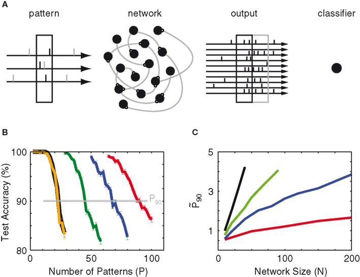
Figure 1. Paradigm. (A) Schematic of the classification task. Sensory-evoked spikes (black ticks) from N_in = 10 Poisson processes (3 shown) and spontaneous background spikes (gray) are fed into a recurrent network. The left black box marks the 90-ms snippet that defines the input pattern. Half of the patterns are labeled (+), the other half (−). The network’s output is read-out at the same temporal bin size of 90 ms, either simultaneous to the input pattern (black box on the right) or time-delayed (gray box). The output patterns are translated into population vectors of spike counts and then used to train a linear classifier to distinguish the (+) vectors from the (−) vectors. (B) Example of test accuracy as a function of the number of trained patterns (P) for 10 (orange), 20 (green), 30 (blue), and 40 (red) network neurons without recurrent connections. The black line indicates the accuracy achieved by training on the input patterns (10 spike trains). The number P₉₀ is defined as the number of patterns at which the test accuracy crosses 90%. (C) Network gain ${\tilde{P}}_{90}=P_{90}\left(\text{network}\right)∕P_{90}\left(\text{input}\right)$ as a function of network size N. The black and blue lines show the ${\tilde{P}}_{90}$ values when each pattern is presented only once for background noise levels of 0 and 0.2 Hz, respectively. Training each pattern 10 times for different realizations of 0.2 Hz noise gives the green line. Finally, training each pattern 10 times at 2 Hz background noise results in the red line.

To quantify the information transmission by the neuronal network, we assess the discriminability of the network activity patterns by an artificial linear classifier (Sonnenburg et al., 2010). The classifier is trained to perform a binary classification task on rate patterns, which are generated by counting the spikes in time bins that match the duration of an input pattern (Figure 1A). The read-out of network activity is delayed with respect to the presentation of the respective input patterns, accounting for the latency induced by the feed-forward synaptic connections. Further details of our model are described in the Materials and Methods section.

For each experiment, we begin by first feeding P input patterns into the network, followed by training the classifier using the P output vectors from the network. For testing, we shuffle the order of the original input patterns and lay these shuffled patterns over a new background noise. This “test input” is then streamed into the same network for a new set of output vectors, and the accuracy at which the previously trained classifier identifies the class labels of these new output vectors is the quantity we use to gauge the network’s capacity to encode temporal input patterns. For benchmarking, we also perform the same experiment without the network, i.e., training and testing the classifier directly over the input vectors.

First examples of testing results (for an uncoupled network with noise-free input) are shown in Figure 1B to illustrate the effect of dimensional expansion. Although the number N_in of dimensions of the input is fixed (at 10), its projection onto a multitude of network nodes provides more dimensions in which linear separation between patterns is possible. At a network size N = 10, the network’s test accuracy is the same as that of the input patterns, which is expected as there is no dimensional expansion. As the network size increases, the computational capacity improves. To quantify this improvement we take the number of patterns P at which the test accuracy crosses 90%, a quantity we call P₉₀. The true gauge of the network’s ability to transmit information is its relative capacity as compared to that of the input. For this purpose we also define the normalized capacity ${\tilde{P}}_{90}=P_{90}\left(\text{network}\right)∕P_{90}\left(\text{input}\right)$ (Figure 1C), which shows a linear relation between capacity and network size with slope 1/N_in. This slope indicates that the fraction α = P₉₀/N for the network patterns is identical to that for the input. In other words, our feed-forward connections provide a plain dimensional expansion of the input, without changing the nature and quality of the code.

As a next step we add noise to the input and observe that the slightest presence of background noise degrades the mean mutual information of both the input and the network (blue line in Figure 1C). One notices that the network is actually more negatively impacted by the presence of noise than the input, and hence a larger network size is required to achieve the same value of ${P̃}_{90}.$ When also including repetitions during the training phase with different background noise, the adverse effect of the noise can be mitigated (green line in Figure 1C). In what follows we use as a default input setup a background noise level of 2 Hz and 10 repetitions of each stimulus during training (red line), unless otherwise noted. The reason is that low capacities (as resulting from increased background noise) require less computational resource, as fewer patterns have to be trained and tested.

Inhibitory Recurrency

As the goal of this work is to use the designed input streams to study the effect of recurrence, we next investigate the effect of the synaptic weight of a homogeneously connected inhibitory network. The synaptic weight is tuned in arbitrary units of w (see Materials and Methods), which are normalized such that the total amount of inhibition received per neuron is invariant to the size and connectivity of the network (see Materials and Methods). Figures 2A–C show spike rasters for different inhibitory weights. Not surprisingly, inhibition suppresses the overall activity. More importantly, as the network inhibition increases, one observes the network’s discrimination performance reaching a maximum, which is ∼30% larger than the performance of the purely feed-forward network (Figure 2D). At the optimal weight, this 30% improvement roughly remains for all different network sizes (Figure 2E).

FIGURE 2

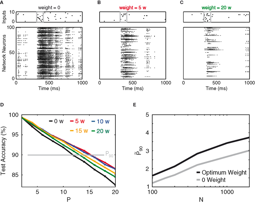
Figure 2. Recurrent inhibition. (A) An example of a default input stream and the network’s response at 0 inhibitory synaptic weight. The input pattern (10 Hz) is contained within the gray box, over ubiquitous background noise (2 Hz). (B,C) Input stream and network response for inhibitory synaptic weights of 5 and 20 w, respectively. (D) Test accuracy vs. P, for network weights of 0 (black), 5 w (red), 10 w (blue), 15 w (orange), and 20 w (green). The read-out of the network patterns is time-delayed by 30 ms as compared to the input. (E) Network gain ${\tilde{P}}_{90}$ as a function of N for optimum weight (5 w, black) and the 0 weight (gray).

Binary Mutual Information

To discover the mechanistic explanation underlying the optimum weight, we study the mean mutual information of the network neurons as a function of synaptic weight (see Materials and Methods). The expectation is that the mean mutual information, as a function of network synaptic weight, would also exhibit a peak similar to that shown in Figure 3A. However, computing the mean mutual information (MI) per neuron as a function of synaptic weight, based on the network’s outputs (Figure 3B), does not show a maximum. Also the average MI per neuron for the top-10 information-rich neurons shows no peak, which excludes that the optimum from Figure 3A just reflects the most informative subset of neurons. Both curves merely seem to reflect the fact that, as inhibitory weight increases, the overall activity of the network decreases, and hence also the entropy of the rate patterns decreases.

FIGURE 3

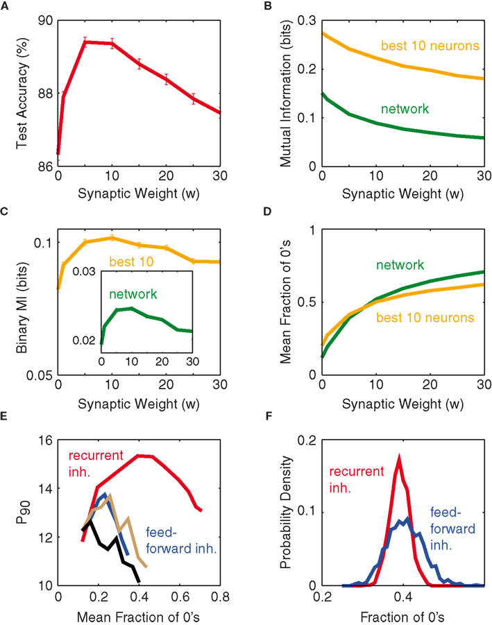
Figure 3. Optimum weight correlates with binary composition of patterns. (A) Test accuracy as a function of synaptic weight, for fixed P = 16 and N = 100. (B) Mutual information (per neuron) as a function of synaptic weight: Average over the entire network (green), average over the top-10 information-rich neurons (orange). (C) Binary mutual information (per neuron) vs. synaptic weight, for both the network average (green, inset) and the top-10 average (orange). (D) Mean fraction of silent neurons (zeros), of the entire network (green) and of the top-10 information-rich neurons (orange) as a function of synaptic weight. (E) P₉₀ as a function of network silence fraction, for both recurrent inhibition (red) and feed-forward inhibition delays of 0 (blue), 10 (gray), and 30 ms (black). (F) Distribution of fractions of 0’s across the set of all input patterns for two simulations from (E) at a mean fraction of 0’s of 0.4. All results are obtained for N = 100.

If one instead computes the average cell-wise MI by setting all non-zero values in the network response to 1 (called binary MI), then one arrives at the curves shown in Figure 3C, displaying good qualitative agreement with test accuracy (Figure 3A). This suggests that instead of classifying on the integer values of spike numbers, the classifier mostly distinguishes the network’s output vectors based on whether there is activity or not. From this, one would assume that the optimal network response to a stimulus would fall close to 50% silence, rendering a theoretical maximum of the binary entropy (Dayan and Abbott, 2001). Figure 3D corroborates this hypothesis, showing the optimum to coincide with a fraction of zeros slightly below 0.5. We interpret this optimum silence fraction as most of the pattern-separation occurring along the silent dimensions and little along those with high firing counts. In fact, this optimum occurs at where the entire network fires at roughly the same silence fraction as its most information-rich neurons (green and orange in Figure 3D intersect, at 46% silence). When the network deviates away from this point, its most informative neurons tend to be the ones that fire closest to the optimum fraction. Figure 3D thus suggests a theoretical optimum weight between 5 and 10 w in our setting. However, for the purpose of simplicity, the rest of this work will employ 5 w as the optimum weight, unless otherwise stated.

Another method we have tested to sparsify the population firing is through feed-forward inhibition on a network lacking intrinsic connectivity: upon each incoming spike, an inhibitory synaptic current is activated on each network neuron with some delay after the excitatory synaptic input. Figure 3E examines the network performance of such an approach and compares it to the recurrent network, and the feed-forward inhibition clearly underperforms irrespective of the delay. We interpret this observation as follows. In the optimum case of recurrent inhibition, network neurons are allowed to accumulate input current and fire in response to the excitation, until roughly 50% of the neurons have fired (for each individual input pattern), before the feedback inhibition becomes strong enough to suppress activation of the yet-to-fire neurons. In the case of feed-forward inhibition the deviations from the 50% firing fraction (that is only achieved on average) are stronger over the whole set of input patterns (Figure 3F), since the inhibitory suppression acts independently of the activity that is actually elicited in the network. It thus seems that the ∼50% optimum firing fraction is meaningful only if it results from recurrent inhibitory feedback, whereas producing the same firing fraction via feed-forward inhibition does not convey the same richness of information.

The above results are robust with respect to changes in the inhibitory recurrent connectivity, input connectivity, and input rate (not shown). Also there, the optimal regime is characterized by a fraction of 40–50% silent neurons, with similar P₉₀ values. We should point out that, for higher (lower) input rates, stronger (weaker) synaptic inhibition is needed to achieve the optimum silence fraction. These results suggest that for inhibitory networks, classification will in general perform optimally, if the stimulus-to-network transformation ends up at a “good” binary probability of about one half.

Short-Term Memory

Thus far the network patterns are derived with a time delay of 30 ms reflecting the latency induced by the cellular integration of the inputs (Figure 2). However, as also can be seen from the raster plots in Figure 2, the network activity persists for a little while after each stimulus. As a consequence the (relatively arbitrary) choice of this read-out delay strongly influences the composition of the output vector. To investigate this dependence, we implement a scheme where the read-out of the network’s response to a particular input pattern is performed at various time delays (Figure 4A).

FIGURE 4

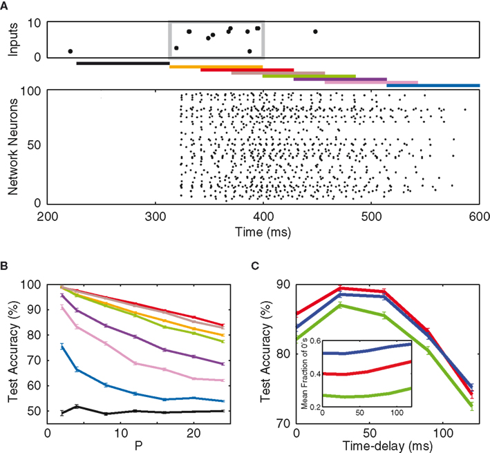
Figure 4. Short-term memory. (A) Top: a typical input raster plot, with 10 Hz input patterns over 2 Hz of background noise. The input pattern is confined within the gray box. Middle: bars of different colors show network read-out time delays of −90 ms (black), 0 ms (orange), 30 ms (red), 60 ms (brown), 90 ms (green), 120 ms (violet), 150 ms (magenta), and 210 ms (blue). Bottom: network response to the input. (B) Test accuracy as a function of P from the aforementioned time delays. (C) Test accuracy (P = 16) as a function of time delay, for synaptic weights of 0 (green), 5 w (red), and 20 w (blue). The optimum time delay stays at approximately 30 ms. Inset: binary composition of the output vectors, as a function of time delay.

The classification results are shown in Figure 4B, and they reveal three important characteristics of our paradigm. Firstly, the time constant (100 ms) of the excitatory post-synaptic currents from the input to the network creates enough excitation in the network such that memory persists more than 200 ms after the presentation of the input pattern. This memory, however, dissipates away before the next pattern is presented (810 ms after the prior pattern). Secondly, one observes the existence of an “optimum time delay” at which the network expresses the most information regarding the inputs. This optimum delay (30 ms), in fact, is approximately independent of the network synaptic weight, as shown in Figure 4C. Lastly, the inset of Figure 4C shows the binary composition of the network’s output, as a function of time delay. One notices that the optimal latency does not coincide with an optimal binary entropy with a fraction of 40–50% silent neurons. The explanation is that, as network read-out is further delayed with respect to the stimulus, the network firing becomes more and more dominated by the background noise. Therefore, unlike the synaptic weight and the input connectivity, the optimal read-out delay is not directly related to the optimal binary entropy, but rather reflects the point in time when the signal-to-noise ratio is highest.

Robustness

Even though the signal-to-noise ratio is highest at the current read-out, what if the signal itself is corrupt? Can a network trained over a set of input patterns still identify them correctly, if the said patterns are slightly mutated? To test robustness against such noise, we perform two experiments: a temporal jitter experiment and a spike-removal experiment. For the jitter experiment, we first construct the training and test inputs as described before, with each pattern repeated 10 times. This time, a temporal jitter is applied to every single spike in a pattern’s time slot. Each jitter is an independently chosen zero-mean Gaussian time shift characterized by the prescribed SD (jitter size). The network is hence trained and tested on these jittered patterns. For the spike-removal experiment, we randomly remove a single spike from each pattern in the training and test inputs.

Figure 5A displays the respective ${P̃}_{90}$ as a function of network size, for several jitter sizes and a single spike removed (11% of the signal on average). We find that all relative capacities ${P̃}_{90}\left(\text{jittered}\right)>1$ and, hence, the network clearly out-performs the input for all values of jitter. Moreover, our results illustrate that, since ${\tilde{P}}_{90}\left(\text{jittered}\right)>{\tilde{P}}_{90}\left(\text{no}\text{jitter}\right),$ the network even protects the information against jitter relative to the input. On the other hand, the removal of spikes from signals deteriorates the network’s performance much more substantially. Nevertheless, the network still out-performs the input.

FIGURE 5

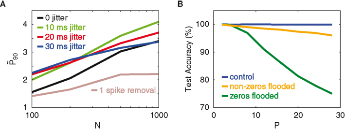
Figure 5. Resistance to jitter. (A) Network gain ${\tilde{P}}_{90}$ as a function of N, for jitter sizes of 0 ms (black), 10 ms (green), 20 ms (red), 30 ms (blue), and the removal of a single spike (purple). The network read-out occurs at a time delay of 30 ms. (B) Test accuracy as a function of P, for a N = 100 with no background noise in the input. About 50% of the network is silent. The lines represent results when one does not alter the test output (blue), floods the non-zeros (firing neurons) of the test output (orange), and floods the zeros (non-firing neurons) of the test output (green). Flooding is done by adding the network’s spike count average per bin to the output vector.

The network’s resistance to temporal jitter can be explained as follows. The classification performance crucially depends on the binary nature of the network spike patterns (Figure 3), which particularly means that the non-spiking neurons contribute considerable information. Since not-spiking is obviously invariant against jitter, this provides a high level of protection against jitter. As a further proof of this hypothesis, we conduct an experiment that looks at the dependence of the classifier on the silent dimensions of the network outputs in performing the classification task. The inputs are a standard set of patterns, without background noise. On average, about 50% of the network’s output vector is silent. During the testing stage, the 0’s of the output vectors are artificially modified with the addition of a positive constant (set to be the network’s average neuronal spike count per time bin). We term this manipulation “flooding.” The aim is to see how much the classifier depends on these flooded neurons to identify trained patterns, by looking at how much the test accuracy is changed relative to the unflooded case. The same experiment, but this time with the non-zeros flooded, is also conducted for comparison. In Figure 5B, the different colors indicate levels of flooding. The key observation is that flooding the zeros in the network pattern dramatically reduces the test accuracy, whereas flooding the non-zeros only mildly reduces it, even though both the zeros and non-zeros constitute half of the output dimensions. This observation corroborates our theory that the network’s computational capacity depends on the binary composition of the network’s activity, which, because of the many non-firing neurons, implies an inherent robustness against temporal jitter.

Mixed Network

As mentioned before, the temporal memory is rather artificially introduced by the very long time constant of the excitatory synaptic inputs. Previous echo-state models, however, generated this temporal memory by excitatory connections within the network (Maass et al., 2002; Jaeger and Haas, 2004; Ganguli et al., 2008; Sussillo and Abbott, 2009). We now also introduce excitatory neurons into the network, with a much shorter excitatory time constant of 20 ms to see which of the findings of the purely inhibitory network still hold in this case.

An example of our mixed network’s response to stimuli is shown in Figure 6A, where the input raster and the read-out delays are analogous to those in Figure 4A. However, a much larger network size is employed due to the sparseness of our mixed network’s connectivity (5%). One can see that the mixed network shows response behavior similar to that of the inhibitory network. After an input pattern, the activity in the network persists for a duration that exceeds the synaptic time constant, and just as in the case of the purely inhibitory network, the best signal-to-noise ratio is obtained at a 30-ms delay (Figure 6B). However, the test performance decays much more steeply with increasing read-out delay, hinting at a reduced short-term memory performance although the activity decays at a similar rate (see Discussion).

FIGURE 6

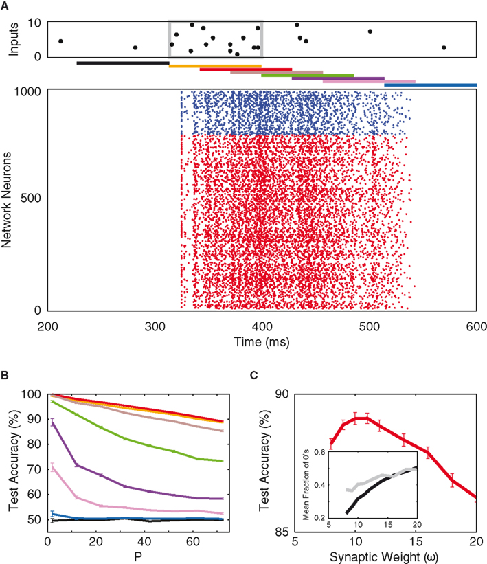
Figure 6. Mixed network. (A) Network response to an example input, and the different time delays for network read-out (as in Figure 4). The network consists of 800 excitatory neurons (red) and 200 inhibitory neurons (blue), with 5% random connectivity. (B) Test accuracy as a function of P for the different time delays [colors as in (A)]. (C) Test accuracy as a function of inhibitory synaptic weight (read-out is time-delayed by 30 ms). Inset: average binary composition of the entire population (black) and of the top-10 information-rich neurons (gray), as a function of inhibitory synaptic weight.

Just like in the purely inhibitory case, the optimum inhibitory synaptic weight (in arbitrary units of ω, see Materials and Methods) and the binary structure of the network’s response as a function of ω (Figure 6C) are determined. In Figure 6C, one sees that, at the optimum weight (10 ω), the network average of silence fraction falls discernibly below that of the purely inhibitory case. This implies that more of the pattern-separation is found along the spiking dimensions of the network (though the most informative neurons still fire close to 50% of the time). Along this line of thought, one would suspect the mixed network’s neurons to fire in a more irregular, non-stereotypic manner such that classification can be made between the non-zero spike counts within each time bin. To further investigate this claim, one needs to take a closer look at the spiking statistics of the two networks.

Figure 7A and its inset compare the two networks’ distributions of inter-spike intervals (ISI) and correlation coefficients (see Methods). Although the mixed network fires at a higher rate (shorter ISI) on average, the coefficient of variation (CV) of its ISI distribution is larger compared to that of the inhibitory network (0.67 vs. 0.48), indicating a longer tail of the ISI distribution and more irregular single-cell firing behavior. At the same time, the neurons in the mixed network fire in a more correlated manner than in the inhibitory network, as one might expect from excitatory network connections.

FIGURE 7

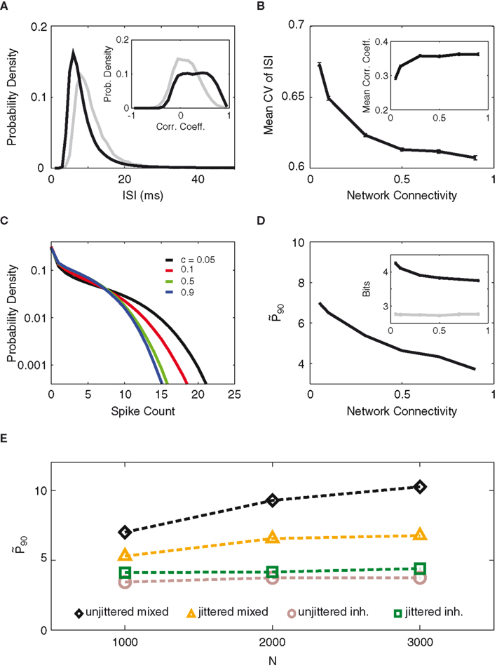
Figure 7. Distinct activity features in mixed vs. inhibitory networks. (A) Distribution of inter-spike intervals (ISI) for the mixed network (black), with 5% connectivity, and the inhibitory network (gray). Inset: distribution of correlation coefficients for the two networks. (B) Average coefficient of variation (CV) and the mean correlation coefficient (Inset) of the mixed network, as a function of network connectivity. The product of connectivity times excitatory weight is kept constant. (C) Distribution of spike counts (per 90 ms bin) for the simulations with excitatory connectivities of 0.05 (black), 0.1 (red), 0.5 (green), and 0.9 (blue) from B. (D) ${\tilde{P}}_{90}$ of the mixed network at different connectivities. Inset: mean entropy of the entire network (gray) and the top-10 entropic neurons (black) as a function of connectivity. (E) ${\tilde{P}}_{90}$ vs. network size for the unjittered mixed network (black, diamond), jittered mixed network (orange, triangle), unjittered inhibitory network (brown, circle), and jittered inhibitory network (green, square). The jitter size is 10 ms. All results are obtained at the optimum weights and read-out delay. In (A–C,E), N = 1000.

While correlations among neurons reduce information content, Figures 7B,C illustrate how the mixed network may still provide superior computational capacity to its inhibitory counterpart. As the connectivity within the mixed network drops the spiking behavior of the neurons becomes increasingly diverse. This is shown by the mean CV of the ISIs (Figure 7B). The increased CV lets us assume that the single-cell spike counts also become more entropic as the connectivity decreases, which we could verify by the increasing width of the spike count distribution (Figure 7C) as well as by the entropy increase of the top-10 most entropic neurons (Figure 7D, inset). As a result of excitatory recurrent coupling, the population patterns are more variable than in the inhibitory network and provide more opportunity for separation between non-zero activity levels. At the same time, the correlation between the neurons falls off steeply with sparser connectivity, reducing the negative impact of correlation on the information content. It should also be pointed out that, within the range of connectivity values experimented, the optimum network silence fraction remains unchanged (not shown).

Lastly, Figure 7E compares the performance and robustness of the two types of network. One first notices that the unjittered mixed network out-performs its inhibitory counterpart by more than a factor of 2. On the other hand, when a small jitter is introduced, the mixed network sees a substantial drop in performance, while the inhibitory network actually becomes better relative to the input. The mixed network’s higher susceptibility to jitter could be ascribed to the correlation between its neurons, in that adverse effects from jittering are propagated by the excitatory neurons to the entire network. Nevertheless, the higher population entropy of the mixed network over-compensates this reduced robustness, as one observes that the mixed network out-performs the inhibitory network also in the case of jitter.

Discussion

We report on a numerical study, in which we have developed a quantitative measure for the gain of linear separability of spatio-temporal spike patterns achieved by a recurrent network. We find that recurrence further improves linear separability as compared to the gain by the non-linear expansion that is already achieved with a non-coupled purely feed-forward network. We address both effects of recurrent inhibition and recurrent excitation. Regarding inhibition, our simulations suggest that, independent of network topology and composition, the neural network’s ability to discriminate temporal spike patterns is optimal so long as the downstream processing produces close to 50% silence (per stimulus) amongst the network neurons. For the excitatory couplings, we observe two effects. First, they realize a short-term memory buffer as activity is retained by traveling through complex high-dimensional trajectories. Second, they improve linear separability of the population patterns by inducing more irregular firing as compared to the purely inhibitory case.

The capacity for short-term memory of an excitatorily coupled network has been shown to strongly depend on the recurrent connectivity of the network (Ganguli et al., 2008): Whereas for normal (e.g., symmetric) coupling matrices, short-term memory only exists if traded with test accuracy, non-normal coupling matrices can achieve memory retention times of order $\sqrt{N}$ even for high test accuracy. The random connectivity matrices used in our simulation are not strictly normal but contain a large normal component according to the central limit theorem. It is therefore not surprising that the accuracy values in Figure 6B drop off rather quickly with read-out time delay. A simple example for non-normal connectivity matrices are realized by sequence-replaying networks (Abeles, 1991; Leibold and Kempter, 2006), in which network activity is made out of self-sustained sequences of patterns. The general problem with non-normal matrices is that the high retention times only can be achieved if the network is properly addressed by the input structure. For the example of the sequence-replaying network, this means that the sequence has to be started at some point. This requires that the feed-forward weights are adjusted to the expected stimuli according to some learning rule. Since in our model, we do not assume any prior knowledge of the input patterns, generating such sequence-replaying networks does not necessarily produce better classification performance.

Our results pertain to the field of reservoir computing (RC), a biologically inspired branch of machine learning (Lukosevicius and Jaeger, 2009). Our paradigm of input/network/read-out is very similar to RC studies, which have proposed a variety of network topologies (Watts and Strogatz, 1998; Barabasi and Albert, 1999; Maass et al., 2002; Haeusler and Maass, 2007) and learning schemes (Lazar et al., 2009; Sussillo and Abbott, 2009) to improve the computational capacity and robustness of artificial neural networks. Specifically, plasticity of recurrent connections has been shown to generate network patterns that are optimal for a fixed pre-defined set of inputs (Lazar et al., 2009; Sussillo and Abbott, 2009). A natural extension of our framework would thus be to train not only the classifier but also include synaptic learning rules for the recurrent connections intending to optimize recurrent processing to the selected set of input patterns.

A classical way of learning recurrent weights is to use a Hebbian weight matrix as suggested in Hopfield (1982), which result in attractor dynamics. The function of such networks is error correction by pattern completion, and short-term memory. These features, however, come at the price of much lower capacity, because their capacity (number of attractors) is subject to dynamical constraints of the network, whereas in the framework of dynamical reservoirs (like in our model) the capacity is only determined by linear separability. Moreover, attractor networks are less suitable for real-time computations owing to the time required to converge to the attractor (Maass et al., 2002).

As a biological motivation, we consider the auditory pathway, which translates the temporal code of the auditory nerve into the sparse rate code of the auditory cortex (Hromádka et al., 2008), or at least relaxes the required temporal precision of cortical processing to the time scale of tens of milliseconds. This translation between time and rate representation is assumed to gradually occur along the multiple processing centers in the auditory brainstem (Joris et al., 2004). A central stage in the ascending auditory pathway is taken by the auditory midbrain, i.e., the inferior colliculus (IC), which collects almost all afferent projections and transfers them to the thalamo-cortical system (Winer and Schreiner, 2005). In this sense the IC acts as a hub, meaning that all auditory information that has to be processed by cortical centers has to be represented in the IC.

While detailed understanding of the inferior colliculus circuit is still elusive, anatomical studies have shown massive convergence of parallel auditory pathways at the IC, recurrent synaptic connections (Huffman and Henson, 1990), as well as a rich array of projections from the IC to the higher auditory centers (Winer and Schreiner, 2005), suggesting that the IC is a central processing unit, responsible for the integration, transformation, and redistribution of auditory information. It is there where maximum discriminability and robustness are desired. As an analogy to our simulation paradigm, the recurrent network would represent the IC, and the input stream would correspond to the ascending pathways connecting to the IC. The key for this network is then to translate the spike trains of these pathways into easily separable population rate patterns that would then be read-out by the thalamo-cortical system.

Our representation of the thalamo-cortical system warrants some discussion. For simplicity, we employ a linear classifier as a stand-in for this unmodeled, highly complex circuitry. While it is clear that the thalamo-cortical system does not merely perform linear classification (e.g., Otazu and Leibold, 2011), the extraction, and discrimination of relevant sensory cues by the cortex requires them to be neuronally represented upstream in a discriminable way. We chose to use linear separability as a benchmark for discriminability, because it can be most easily represented by neural elements and requires the least assumptions about the read-out structure. The linear classifier is therefore mainly used as a means for quantifying discriminability and not meant to be a direct biological representation of latter-stage auditory information processing. Moreover, the choice of a two-class classification task can easily be generalized as one may simply tack on more binary read-out units for multi-class differentiation, as necessary, e.g., in speech recognition.

Based on our findings, and assuming the population code in the IC to be optimized for linear discrimination, the many intrinsic synaptic connections of the IC could serve to maximize entropic firing and minimize neuronal correlation. This translates to sparse connectivity amongst the excitatory neurons, strongly varying inter-spike intervals, and firing patterns that are somewhat below 50% silence per downstream integration time window.

Materials and methods

Neuron Model

For our neuronal model, we use the integrate-and-fire neuron with exponentially decaying post-synaptic current from the Neural Simulation Technology (NEST) Initiative software package, version 2.0 (Gewaltig and Diesmann, 2007). The simulations are run at a time resolution of h = 0.1 ms. The membrane capacitance is C = 250 pF. Resting potential is −70 mV. The spike threshold is set to V_th = −55 mV. After a spike the voltage is reset to the resting potential. The neurons have a refractory time of t_ref = 2 ms and a membrane time constant of τ_m = 10 ms.

Synapse Model

Synaptic currents are modeled as exponentially decaying with time constant of 8 ms for inhibition. Feed-forward excitation decays at a time constant of 100 ms for purely inhibitorily coupled networks, and at a time constant of 20 ms for the mixed networks, which is the same as for the excitatory recurrent synapses.

For the inhibitory network, excitatory feed-forward weights result in a current amplitude of 500 pA. Inhibitory synaptic weights are given in units of w = −200 pA/(N × c), where c is the network connectivity and N is the network size, such that the total amount of inhibition received per neuron is invariant to the size of the network.

For the mixed network the excitatory feed-forward weights generate an amplitude of 400 pA, and the recurrent excitatory synapses generate an amplitude of I_exc,_R = 800 pA/(N × p × c), where p is the fraction of the excitatory neurons in the network. The inhibitory weight is tuned in units of ω = −I_exc,R.

All synaptic transmissions introduce an additional delay of 1 ms.

Input Scheme

For our linear classification task, half of the input patterns are randomly picked to be placed under the (+) label, with the other half under the (−) label. A schematic of an input pattern is shown in the first panel of Figure 1A. For all of our simulations, we use 90 ms time bins and 10 Hz spike rates to construct the input patterns. The spacing between the input patterns is fixed at 810 ms.

Network Topography

The inputs are feed-forwardly directed to a network of N integrate-and-fire neurons. Each input is randomly connected to exactly 50% of the network neurons, for both the inhibitory network and the mixed network. Each network neuron is connected to N × c other network neurons. That means not only does the neuron have the possibility of connecting to itself, but its number of connections also varies according to binomial statistics with expectation value N × c.

The network connectivity, c, differs between the inhibitory network and the mixed network. For our inhibitory network, we set c = 100% by default. For our mixed network, we use c = 5% throughout.

Linear Classifier

As a linear classifier we use the LIBSVM support vector machine implementation provided by the SHOGUN machine learning toolbox (Sonnenburg et al., 2010). We have also employed a self-programmed Perceptron and obtained the same results.

Mean Mutual Information

We compute the mean mutual information of our network response from the averaged marginal entropies. If the variable r represents the spike count per bin of a neuron, then the mean response entropy per neuron is computed as

$H=-\frac{1}{N}\sum _{i=1}^N\sum _r{P}_i\left[r\right]{log}_2{P}_i\left[r\right],$(1)

where N is the total number of network neurons, and P_i[r] is the probability of occurrence of r for the ith neuron, computed over all output vectors.

If r(+) denotes a neuron’s response to a class label (+) stimulus, and r(−) to a class label (−) stimulus, then the mean noise entropy is

$\begin{array}{rcll}{H}_{\text{noise}}& =-\frac{1}{2N}\sum _{i=1}^N\sum _r{P}_i\left[r\left(+\right)\right]{log}_2{P}_i\left[r\left(+\right)\right]& & \\ & -\frac{1}{2N}\sum _{i=1}^N\sum _r{P}_i\left[r\left(-\right)\right]{log}_2{P}_i\left[r\left(-\right)\right],& & \text{(2)}\end{array}$

and our mean mutual information per neuron is computed as

$I_m=H-H_{\text{noise}}$(3)

Correlation coefficient

The correlation coefficients between pairs of neurons are computed as follows. First, the spike counts of each network neuron, in response to the entire set of input patterns, are collected into a vector. Then the correlation coefficient between each pair of neurons is simply the correlation coefficient between their respective spike count vectors. In addition, when computing the mean correlation coefficient of the entire network, only absolute values are considered.

The authors are grateful to Nikolay Chenkov for help at a preliminary stage of the study and comments on the manuscript, Matus Simkovic for help at a preliminary stage of the study, and Kay Thurley for comments on the manuscript. This work has been supported by the German ministry of education and research (BMBF) under grant numbers 01GQ0440 (Bernstein Center for Computational Neuroscience) and 01GQ0981 (Bernstein Fokus Neural Basis of Learning).

Conflict of Interest Statement

The authors declare that the research was conducted in the absence of any commercial or financial relationships that could be construed as a potential conflict of interest.

References

Abeles, M. (1991). Corticonics. Cambridge: Cambridge University Press.

Barabasi, A.-L., and Albert, R. (1999). Emergence of scaling in random networks. Science 286, 509–512.

Pubmed Abstract | Pubmed Full Text | CrossRef Full Text

Ben-Yishai, R., Bar-Or, R. L., and Sompolinsky, H. (1995). Theory of orientation tuning in visual cortex. Proc. Natl. Acad. Sci. U.S.A. 92, 3844–3848.

Pubmed Abstract | Pubmed Full Text | CrossRef Full Text

Dayan, P., and Abbott, L. F. (2001). Theoretical Neuroscience. Cambridge, MA: MIT Press.

Ganguli, S., Huh, D., and Sompolinsky, H. (2008). Memory traces in dynamical systems. Proc. Natl. Acad. Sci. U.S.A. 105, 18970–18975.

Pubmed Abstract | Pubmed Full Text | CrossRef Full Text

Gewaltig, M.-O., and Diesmann, M. (2007). NEST (neural simulation tool). Scholarpedia 2, 1430.

CrossRef Full Text

Haeusler, S., and Maass, W. (2007). A statistical analysis of information-processing properties of lamina-specific cortical microcircuit models. Cereb. Cortex 17, 149–162.

Pubmed Abstract | Pubmed Full Text | CrossRef Full Text

Hopfield, J. J. (1982). Neural networks and physical systems with emergent collective computational abilities. Proc. Natl. Acad. Sci. U.S.A. 79, 2554–2558.

Pubmed Abstract | Pubmed Full Text | CrossRef Full Text

Hromádka, T., DeWeese, M. R., and Zador, A. M. (2008). Sparse representation of sounds in the unanesthetized auditory cortex. PLoS Biol. 6, 124–137.

CrossRef Full Text

Huffman, R. F., and Henson, O. (1990). The descending auditory pathway and acousticomotor systems: connections with the inferior colliculus. Brain Res. Rev. 15, 295–323.

CrossRef Full Text

Jaeger, H., and Haas, H. (2004). Harnessing nonlinearity: predicting chaotic systems and saving energy in wireless communication. Science 304, 78–80.

Pubmed Abstract | Pubmed Full Text | CrossRef Full Text

Joris, P. X., Schreiner, C. E., and Rees, A. (2004). Neural processing of amplitude-modulated sounds. Physiol. Rev. 84, 541–577.

Pubmed Abstract | Pubmed Full Text | CrossRef Full Text

Lazar, A., Pipa, G., and Triesch, J. (2009). SORN: a self-organizing recurrent neural network. Front. Comput. Neurosci. 3:23.

CrossRef Full Text

Leibold, C., and Kempter, R. (2006). Memory capacity for sequences in a recurrent network with biological constraints. Neural Comput. 18, 904–941.

Pubmed Abstract | Pubmed Full Text | CrossRef Full Text

Linkser, R. (1986). From basic network principles to neural architecture: emergence of orientation columns. Proc. Natl. Acad. Sci. U.S.A. 83, 8779–8783.

Pubmed Abstract | Pubmed Full Text | CrossRef Full Text

Lukosevicius, M., and Jaeger, H. (2009). Reservoir computing approaches to recurrent neural network training. Comput. Sci. Rev. 3, 127–149.

CrossRef Full Text

Maass, W., Natschlaeger, T., and Markram, H. (2002). Real-time computing without stable states: a new framwork for neural computation based on perturbations. Neural Comput. 14, 2531–2560.

Pubmed Abstract | Pubmed Full Text | CrossRef Full Text

Otazu, G. H., and Leibold, C. (2011). A corticothalamic circuit model for sound identification in complex scenes. PLoS ONE 6, e24270.

CrossRef Full Text

Popper, A. N., and Fay, R. R. (1992). The Mammalian Auditory Pathway: Neurophysiology. Heidelberg: Springer.

Sonnenburg, S., Raetsch, G., Henschel, S., Widmer, C., Behr, J., Zien, A., de Bona, F., Binder, A., Gehl, C., and Franc, V. (2010). The SHOGUN machine learning toolbox. J. Mach. Learn. Res. 11, 1799–1802.

Sussillo, D., and Abbott, L. F. (2009). Generating coherent patterns of activity from chaotic neural networks. Neuron 63, 544–557.

Pubmed Abstract | Pubmed Full Text | CrossRef Full Text

von der Malsburg, C. (1973). Self-organization of orientation sensitive cells in the striate cortex. Biol. Cybern. 14, 85–100.

CrossRef Full Text

Watts, D. J., and Strogatz, S. H. (1998). Collective dynamics of ‘small world’ networks. Nature 393, 440–442.

Pubmed Abstract | Pubmed Full Text | CrossRef Full Text

Winer, J. A., and Schreiner, C. E. (2005). The Inferior Colliculus. New York, NY: Springer.

Zhang, K. (1996). Representation of spatial orientation by the intrinsic dynamics of the head-direction cell ensemble: a theory. J. Neurosci. 16, 2112–2126.

Pubmed Abstract | Pubmed Full Text