Fluctuating inhibitory inputs promote reliable spiking at theta frequencies in hippocampal interneurons

Introduction

Brain rhythms of different frequencies are known to be correlated with different behavioral states (Buzsáki and Draguhn, 2004). In particular, theta-frequency (4–12 Hz) rhythms in the hippocampus, which occur during active, exploratory states, play important roles in learning and memory. These rhythms occur with the most regularity and the largest amplitude in the stratum lacunosum-moleculare of the hippocampal CA1 region (Buzsáki, 2002). Although a precise understanding of how theta rhythms are generated in network circuitry does not exist, it is clear that the characteristics of inhibitory cells, or interneurons, are critically important. However, interneurons exhibit a high level of diversity in their cellular characteristics, which makes understanding the contributions of any given interneuron type a challenge (Klausberger and Somogyi, 2008).

Experiments determining cellular, biophysical details of interneurons are necessarily done in vitro where the behavior of isolated cells can be explored. However, in vitro and in vivo environments are different and it is not obvious how characteristics displayed in vitro are manifested in vivo. This can be addressed to a degree by using dynamic clamp methodologies to create in vivo-like situations in the dish or by imposing synaptic background activities that mimic in vivo-like scenarios onto model cells (Destexhe et al., 2003). For example, Fernandez and White (2008) used a dynamic clamp protocol on stellate cells of the entorhinal cortex to examine subthreshold theta oscillations and spiking dynamics in an in vivo context. Their results suggest that linking cellular properties to network behavior requires consideration of in vivo-like conditions as different biophysical mechanisms are brought to bear. Such studies indicate that imposing in vivo-like conditions on biophysical model cells or on biological cells in vitro is a strategy that is helpful to obtain an understanding of the contributions of different interneuron types.

Of the many diverse interneuron types in the hippocampus, we focus here on CA1 interneurons located at the stratum lacunosum-moleculare and radiatum junction (LM/RAD). These neurons display subthreshold membrane potential oscillations (MPOs) at theta frequencies in vitro (Chapman and Lacaille, 1999a), and as such, may contribute to generating population theta oscillations. They express cholecystokinin (CCK) and calbindin (CB) and synapse onto dendritic locations (Williams et al., 1994; Chapman and Lacaille, 1999a,b; Bourdeau et al., 2007). With these characteristics, they may be Schaffer collateral-associated interneurons as described by Vida (2010). The complement of potassium channels in these cells has been characterized allowing for a biophysically based model to be developed (Morin et al., 2010). With the constrained biophysics, the model is able to produce MPOs as observed experimentally. Experimental work has emphasized the importance of A-type potassium currents in the generation of these MPOs since Kv4.3 is expressed in LM/RAD cells, and A-type currents and MPOs are impaired when expression of Kv4.3 is prevented (Bourdeau et al., 2007). Our modeling work supports this as well as indicating an essential role for persistent sodium currents in MPO generation (Morin et al., 2010). These LM/RAD interneurons are thought to contribute to hippocampal theta population activities by rhythmically pacing pyramidal cells with inhibitory postsynaptic potentials (IPSPs). In vitro cholinergic induction of MPOs in LM/RAD interneurons was shown along with the firing of these cells to be able to pace the pyramidal cell population (Chapman and Lacaille, 1999b).

The ability of LM/RAD cells to exhibit reliable theta spiking in vivo would suggest that they can pace the pyramidal cell population and contribute to population theta rhythms. By reliability, we invoke the definition given in Ermentrout et al. (2008) which considers reliability as “the degree to which a neuron fires the same number of action potentials, at the same time, in response to repeated delivery of the same input,” and we further impose a theta spiking frequency range given our context. In this paper we ask two questions: (i) Can LM/RAD cells fire reliably at theta frequencies in vivo, and if so, (ii) what biophysical properties and network conditions support this? We address these questions computationally by applying in vivo-like conditions to our developed model interneurons. Using the reliability measure of Schreiber et al. (2003), we find that reliability measure values of 0.1 show clear repeatability across trials at theta frequencies. Thus, reliable theta spiking can occur in LM/RAD model cells with appropriate biophysical characteristics under in vivo-like scenarios. This supports the possibility that LM/RAD cells can contribute to population theta rhythms. Interestingly, we find that reliable theta spiking is promoted when synaptic background activities emphasize inhibitory fluctuations. Therefore, we suggest that the balance of synaptic input to LM/RAD cells should be more heavily weighted toward inhibition if they are to be able to contribute to population theta activities.

Materials and Methods

Hippocampal Interneuron Model (“in vitro”)

A single compartment model of an LM/RAD interneuron developed by Morin et al. (2010) is adapted in this study to computationally analyze the spiking behavior of this neuron type. The model includes two types of voltage-gated sodium currents, four types of voltage-gated potassium currents, leak current, and a noise term that is taken to be intrinsically generated. The current balance is given by:

$C\frac{dV}{dt}=I_{\text{DC}}-\left(I_{\text{leak}}+I_{\text{gate}}+I_{\text{NaT}}+I_{\text{NaP}}+I_{\text{FDR}}+I_{\text{SDR}}+I_{\text{D}}+I_{\text{A}}\right)$(1)

Parameter values and equations governing each term are given in Table 1. The experimental data and rationale that underlie these model details are provided in Morin et al. (2010). I_DC is a control parameter representing injected current into the model interneuron, mimicking what was done experimentally. The inclusion of the noise term, I_gate, in this model (in the form of additive Gaussian white noise), results in MPOs as observed in experiment (Morin et al., 2010) – see Figure 1A. The size of the intrinsic noise term is chosen such that the theta-frequency MPOs produced by the model have magnitudes comparable to experimental values.

TABLE 1

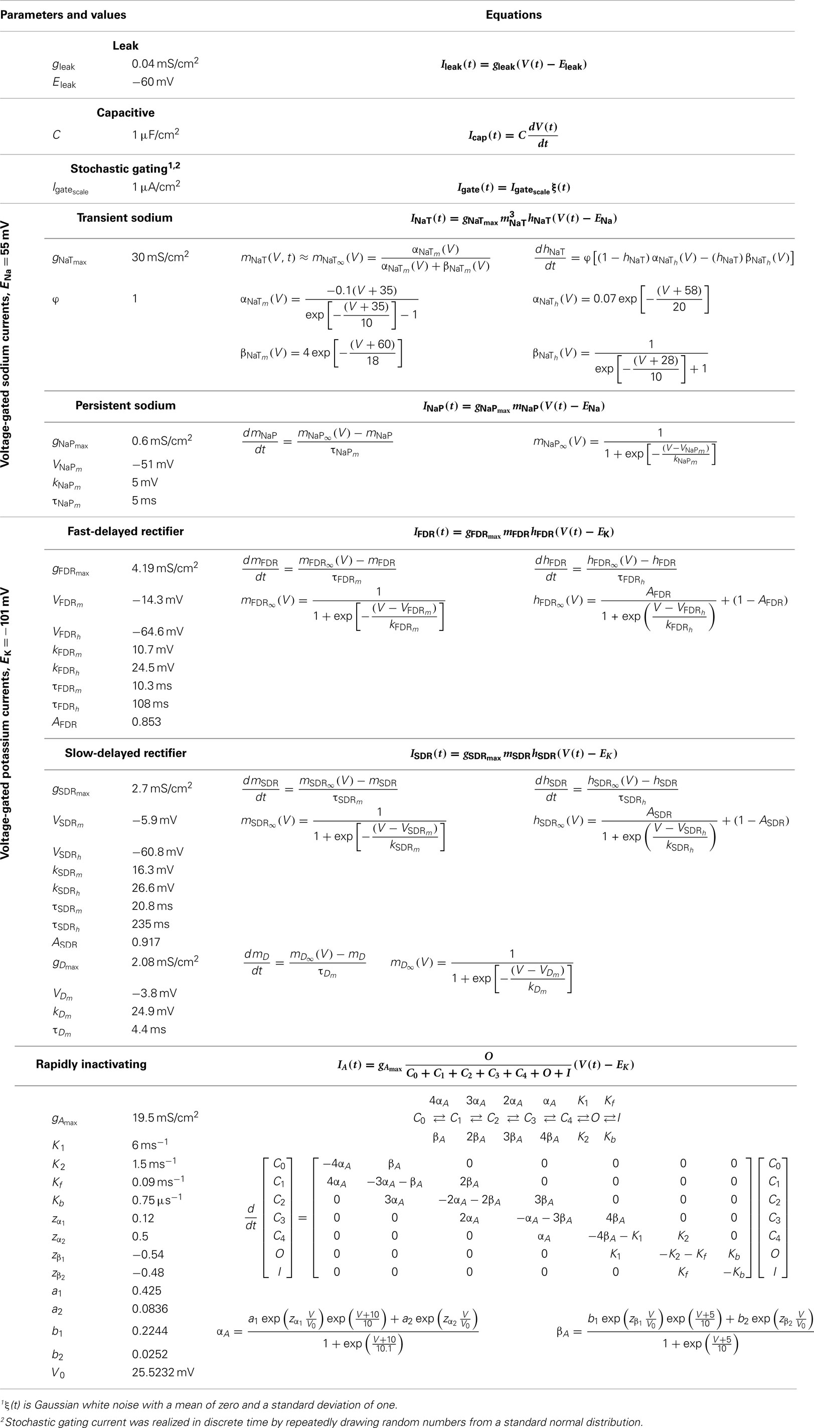
Table 1. Current equations for in vitro LM/RAD cell model.

FIGURE 1

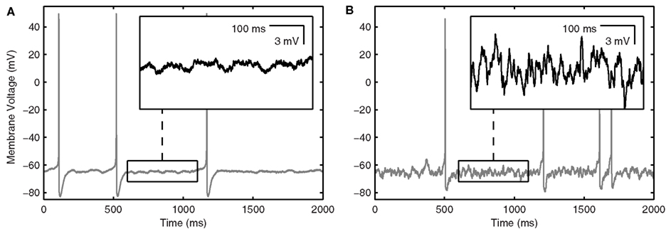
Figure 1. LM/RAD interneuron model output. (A) Sample in vitro voltage waveform from the Standard model variant as in Equation 1 with I_DC = 6.82 μA/cm². Inset: Enlargement of voltage trace showing MPOs as observed experimentally. (B) Sample in vivo voltage waveform from the Standard model variant as in Equation 2 with I_cholinergic = 0.175 μA/cm², μ_exc = 0.14 mS/cm², μ_inh = 0.26 mS/cm², σ_exc = 0.02 mS/cm², σ_inh = 0.03 mS/cm², I_probe = 0 μA/cm². Inset: Enlargement of voltage trace showing increased baseline fluctuations as would occur in vivo.

Intrinsic noise is included in the LM/RAD model to represent the inherent noisy behavior of the isolated cell, generating MPOs as seen in experiment. Since all synaptic input is blocked, the noisiness can only be due to intrinsic properties and thus the noise term is taken to represent stochastic channel gating. We previously suggested that the generation of MPOs is due to a generic critical slowing mechanism in which there is an increase in the response of a system to noisy input as the system is brought toward threshold (Steyn-Ross et al., 2006; Morin et al., 2010). Thus the intrinsic noise in the system brings about an amplitude increase in MPOs with depolarization, as observed experimentally. We have noted that amplitude increases in subthreshold oscillations occur in other systems (entorhinal cortex stellate cells) suggesting that the critical slowing mechanism may be general (Skinner, 2012). We note that although more sophisticated forms of noise were investigated in our in vitro model, the choice of representation did not preclude a generic critical slowing mechanism from potentially being in play. Although the mechanism is generic, it is the model specifics that allow such an enhanced response (i.e., MPOs) to occur – there needs to be appropriate balances and kinetics in the biophysical currents so that the rate and range of the model system can bring about theta-frequency MPOs. We found that while the A-type potassium current, I_A, plays more of a role in determining the frequency of MPOs, the persistent sodium current, I_NaP, is essential in allowing MPOs to occur in the first place, by creating a slow enough rate transition as the system approaches threshold (Morin et al., 2010).

Model Variants

Five variants of the model LM/RAD interneuron are created with different maximum conductance values for I_A and I_NaP. These currents are targeted because they are instrumental in modulating the subthreshold fluctuations and determining the voltage range over which MPOs occur (Morin et al., 2010). The variants have maximum conductances $\left(g_{{\text{A}}_{max}},g_{\text{Na}{\text{P}}_{max}}\right)$ of (19.5, 0.6), (0, 0.6), (39, 0.6), (19.5, 0.3), and (19.5, 0.9) mS/cm² and are named “Standard,” “A0,” “A200,” “NaP50,” and “NaP150” respectively, according to their conductance percentages relative to the Standard model. These conductance values are identical to the variations used in Morin et al. (2010) allowing for a parallel understanding of how neuronal membrane resonance (a subthreshold phenomenon explored in that study) established by conductance balances modulates inputs to the neuron to influence its spiking characteristics (a suprathreshold phenomenon that is explored here).

Extended Model (“in vivo”)

We consider an extended model in this study that inherits all the features of the in vitro model but simulates an in vivo network situation by including cholinergic input and synaptic currents (see Figure 2 for schematic). In other words, our model is of a virtual network. The current balance for the extended model is given by:

$\begin{array}{rcll}C\frac{dV}{dt}& =\left(I_{\text{cholinergic}}-I_{\text{exc}}-I_{\text{inh}}+I_{\text{probe}}\right)& & \\ & -\left(I_{\text{leak}}+I_{\text{gate}}+I_{\text{NaT}}+I_{\text{NaP}}+I_{\text{FDR}}+I_{\text{SDR}}+I_{\text{D}}+I_{\text{A}}\right)& & \text{(2)}\end{array}$

FIGURE 2

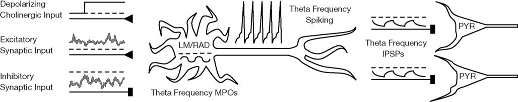
Figure 2. Schematic of network scenario for LM/RAD model interneurons. LM/RAD cells, which display intrinsic MPOs at theta frequencies, need to spike reliably at theta frequencies in order to contribute to hippocampal theta rhythms by rhythmically pacing pyramidal cells (PYR) with their IPSPs. This reliable theta spiking needs to occur in a network environment where the cell receives cholinergic and synaptic input.

Additional equations and parameters for the extended model are given in Table 2, and described in more detail below. A sample voltage trace from this in vivo-like model is shown in Figure 1B.

TABLE 2

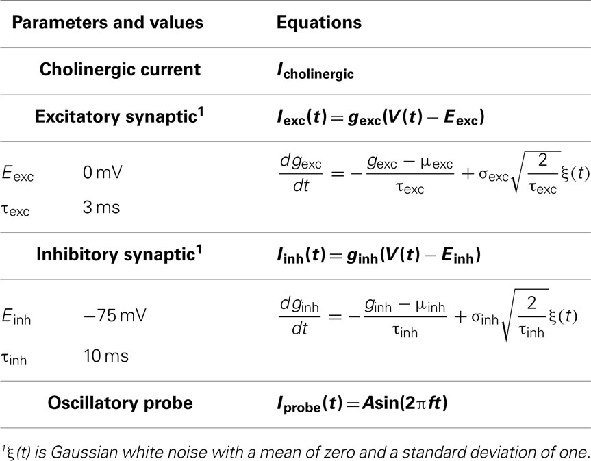
Table 2. Additional currents in extended LM/RAD in vivo cell model.

Cholinergic input

Cholinergic afferents from the medial septum synapse onto both CA1 pyramidal cells and LM/RAD interneurons (e.g., see Figure 6 of Chapman and Lacaille, 1999b). Application of the cholinergic agonist carbachol depolarizes hippocampal inhibitory interneurons in vitro to induce MPOs (Chapman and Lacaille, 1999b) and spiking. This suggests that cholinergic input from the medial septum may bring interneurons near threshold in vivo. In this study, we treat cholinergic input from the medial septum, I_cholinergic, as a depolarizing DC current of tunable magnitude. We use this simple representation since many of the details required to model the kinetics of particular acetylcholine receptors are unclear at this time.

Synaptic background activity

Synaptic background activity is included to represent the model cell in a virtual network scenario. This activity is modeled by incorporating excitatory and inhibitory currents, I_exc and I_inh respectively, and treating the synaptic conductances as stochastic elements instead of the synaptic currents themselves. The advantage of this approach is that it allows membrane voltage dynamics to influence the synaptic currents and permits straightforward identification of high-conductance states (Destexhe, 2007). Destexhe et al. (2001) modeled synaptic conductances using a single-variable, mean-reverting Ornstein–Uhlenbeck stochastic process and provided a discretization accounting for step size that we adopt. These processes require knowledge of the synaptic reversal potentials (E_exc, E_inh) and fluctuation time constants (τ_exc, τ_inh) but allow the mean (μ_exc, μ_inh) and standard deviation (σ_exc, σ_inh) of the synaptic conductances to be treated as free parameters. The same reversal potentials used by Destexhe et al. (2001) are used here (E_exc = 0 mV, E_inh = −75 mV). Piwkowska et al. (2008) fitted theoretical expressions derived from an Ornstein–Uhlenbeck based point conductance model of synaptic activity to experimental membrane voltage power spectral densities and found that the fluctuation time constants that produced the best fit were (τ_exc = 3 ms, τ_inh = 10 ms).

Oscillatory probe current

Aside from the mean and standard deviation of the synaptic conductances, which provide a broad definition of the system state (quiescent vs. high conductance), several population frequencies exist in the hippocampus (Buzsáki, 2011). To examine if strong rhythmicity in synaptic input (which may arise from population rhythms) is an important determinant of spike reliability, we include a sinusoidal current, I_probe, with variable amplitude, A, and frequency, f. Since the probe amplitudes used are small (see Model Parameter Ranges), the natural rhythmicity generated intrinsically is not obscured.

Spiking Threshold and Frequency Response of Models

The in vitro hippocampal interneuron model has an intrinsic stochastic component and the extended in vivo-like model has two additional external stochastic components (excitatory and inhibitory conductances). We understand the underlying dynamics of our models by removing the stochastic components and examining the following (deterministic) current balance.

$C\frac{dV}{dt}=I_{\text{DC}}-\left(I_{\text{leak}}+I_{\text{NaT}}+I_{\text{NaP}}+I_{\text{FDR}}+I_{\text{SDR}}+I_{\text{D}}+I_{\text{A}}\right)$(3)

The deterministic model governed by Eq. 3 is injected with a wide range of DC inputs at 1 nA/cm² steps and allowed to evolve for 2.2 s (see Simulation Procedure) for each input step. The first 0.2 s are discarded to eliminate transients and the spikes that occur in the latter 2.0 s are tallied to determine spiking frequencies for different injected currents (f–I curves).

For the Standard, A0, and NaP150 model variants, the spiking frequencies begins at 0 Hz and smoothly increase with increasing depolarization (i.e., DC input) so that it is possible to clearly identify the current values (accurate to within the step size of the DC sweep) at which spiking begins. For the A200 and NaP50 model variants, the f–I curves are more complex to determine as spiking onset is delayed depending on the level of injected current indicating additional (slower) dynamics. As such, we use DC values for which spiking clearly starts at the beginning of the 2.0-s frame to obtain the f–I curves. The f–I curves shown in Figures 3 and 4 are smoothed by interpolating between points.

FIGURE 3

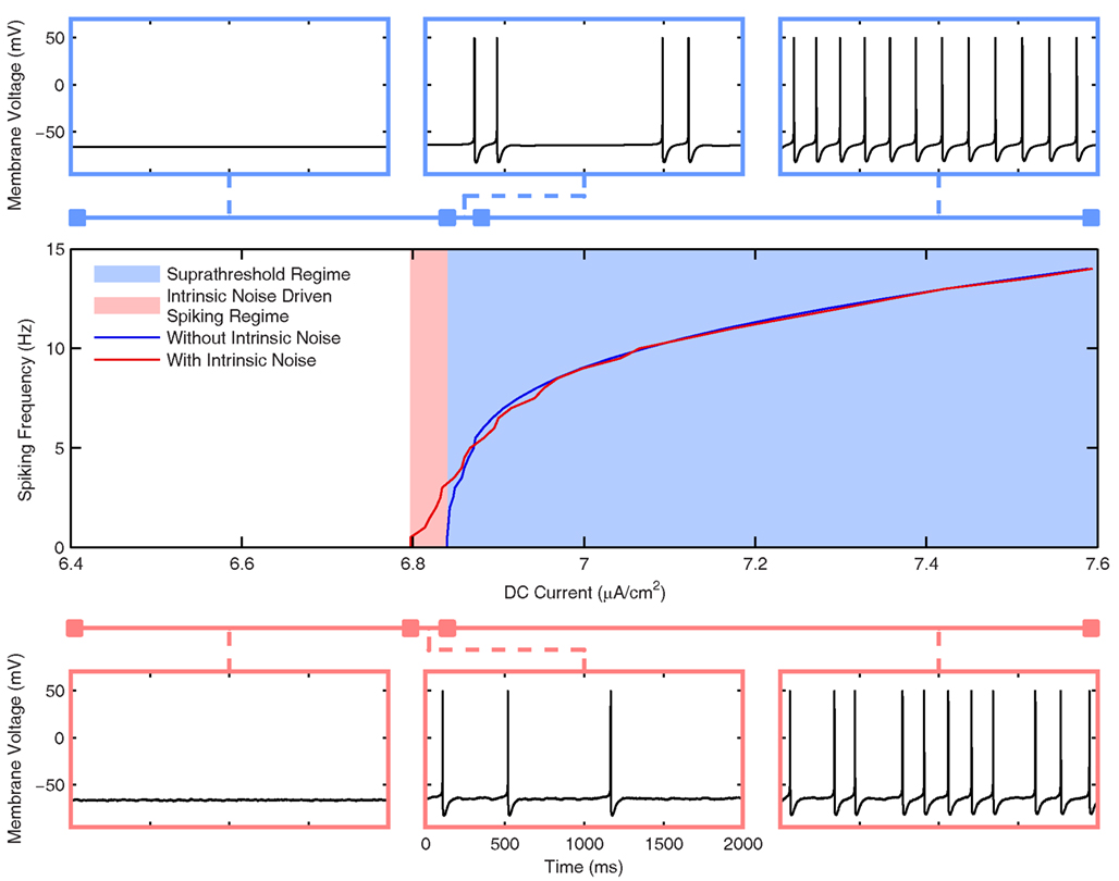
Figure 3. Frequency response of the Standard LM/RAD cell model. (Top Row) Voltage waveforms in the absence of intrinsic noise for I_DC = 6.6, 6.843, and 6.9 μA/cm² (left to right) corresponding to silent, doublet, and regular firing regions respectively. (Bottom Row) Voltage waveforms in the presence of intrinsic noise for I_DC = 6.6, 6.82, and 6.9 μA/cm² (left to right). (Middle) Frequency vs. DC current (f–I) curve in the presence (red) and absence (blue) of intrinsic noise as given by Eqs 1 and 3 respectively. The noiseless f–I curve implies that a Type I-like bifurcation may be present due to the emergence of spiking at a zero frequency but more complex dynamics are also at play as evidenced by the doublet firing.

FIGURE 4

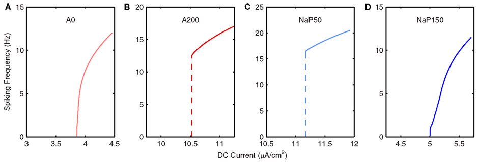
Figure 4. Frequency response of LM/RAD model variants. Frequency vs. DC current (f–I) curves, as given by Equation 3, for (A) A0, (B) A200, (C) NaP50, and (D) NaP150 model variants. Note that A0 and NaP150 model variants have Type I-like characteristics whereas A200 and NaP50 model variants have Type II-like characteristics.

Model Calibration Encompassing and Emphasizing Fluctuation-Driven Regimes

To quantitatively examine model output, we use a spike reliability measure (see Spike Reliability) from Schreiber et al. (2003). Mean-driven and fluctuation-driven firing were examined as distinct mechanisms shaping the reliability of neural responses (Schreiber et al., 2009), where spike reliability is dependent on both spike precision and spike probability. In the mean-driven firing regime, one is above spike threshold so spike reliability is mainly dictated by spike precision in the face of noisy synaptic background activities. However, if one is below spike threshold in the fluctuation-driven regime, then spike reliability can be optimized under certain conditions since spike probability improves with increased noise while spike precision diminishes (see Figure 9 of Schreiber et al., 2009).

Our goal here is not to examine mean and fluctuation-driven regimes per se, but rather to examine our models under in vivo-like conditions which situate the neuron in the vicinity of spike threshold so that fluctuation-driven regimes are of importance. Furthermore, we aim to determine what parameter sets (representing in vivo-like states) may be ideal in bringing about reliable theta-frequency spiking in LM/RAD cells. In turn, such parameter sets could be indicative of the sort of network environment (i.e., inputs being received) that is required for LM/RAD cells to functionally participate in population level theta rhythms. At very depolarized membrane voltages, tonic spiking would result in high reliability values (due to high spike probability) whereas for very hyperpolarized values, the neuron is silent so that the notion of spike reliability is not meaningful – both these regions are fairly predictable and well characterized. Near the spiking threshold however, transient perturbations (due to synaptic bombardments as would occur in vivo) can affect spike reliability in complex ways that are not well characterized. These regions, where fluctuation-driven spiking is important, are likely the relevant regions to consider for in vivo behavior (Destexhe, 2010). To hone into this window around spiking threshold, it is necessary to identify appropriate current and voltage bounds. To this end, and in the absence of a formal bifurcation analysis, we determine voltage calibration (V–I) curves for our models.

The deterministic model governed by Eq. 3 is injected with a wide range of DC currents according to the same procedure used in the determination of the f–I curves. If there is no spiking, the steady-state membrane voltage at the end of the simulation is recorded and used for the V–I curves. If spiking occurs, one cannot unambiguously associate a membrane voltage value to the DC input since a spike could occur at the end time itself, for example. Therefore, the membrane voltage associated with a suprathreshold DC current is defined as the instantaneous membrane voltage, V*, that produces a net transmembrane current that is closest to the DC input as shown (Eq. 4) so that the magnitude of the instantaneous derivative in Eq. 3 is minimized.

$V^{*}=arg\underset{v}{min}|I_{\text{DC}}-\left(I_{\text{leak}}+I_{\text{NaT}}+I_{\text{NaP}}+I_{\text{FDR}}+I_{\text{SDR}}+I_{\text{D}}+I_{\text{A}}\right)|$(4)

For some model variants, there is a sharp increase in the V–I curve (several millivolts) within a few steps of the spiking threshold current value so it is difficult to unambiguously identify voltage values for that narrow current range. Therefore, upper and lower bounds on the threshold voltage values are presented (along with the corresponding range of DC values) in Table 3. For the NaP50 model variant, no choice of V* produces a net transmembrane current to track DC values above that corresponding to the upper threshold voltage, and in fact, the solution to Eq. 4 for all suprathreshold DC currents is the upper threshold voltage itself. Curve fitting is performed on the V–I curves of the five model variants. The best fits are produced by treating the curves as piecewise functions with quadratic subthreshold regions and linear suprathreshold regions.

TABLE 3

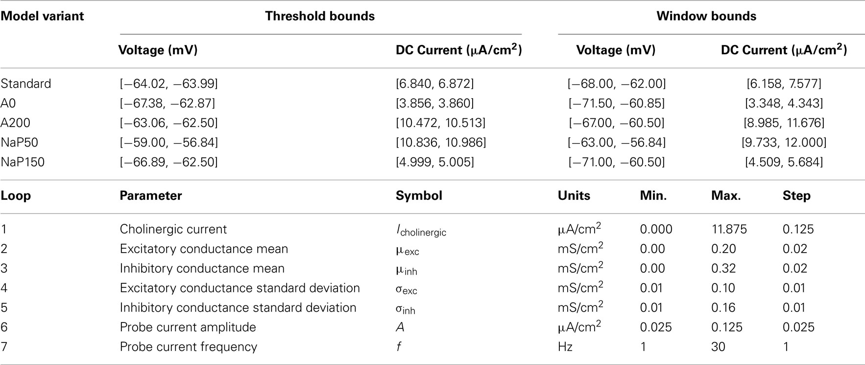
Table 3. Numerics and bounds for parameter sweep.

For each model variant except NaP50, the window of interest around its threshold is defined to be 4 mV below its minimum voltage threshold value to 2 mV above its maximum voltage threshold value to a tolerance of 0.1 mV, as given by the V–I calibration curves. For the NaP50 model variant, it is not possible to achieve voltages above its maximum threshold voltage as described earlier, so its upper bound is defined in terms of applied currents to be roughly 1 μA/cm² above the DC value corresponding to the maximum threshold voltage. The window is not chosen symmetrically around the threshold and is instead biased toward the subthreshold region so that fluctuation-driven spiking can be explored more comprehensively. The size of the window is appropriate because it is the same order of magnitude as the MPOs. The voltage and current ranges used in establishing the window bounds are given in Table 3.

Model Parameter Ranges

The highest sensitivity of the model to changes in parameter values is expected to occur near the spiking threshold since slight perturbations can cause large changes in membrane dynamics (i.e., spiking or not). Therefore, performing parameter sweeps on the model variants within the determined window bounds (see Table 3) is a reasonable way to gauge the sensitivity of spike reliability on the different internal conductances and parameters, and to identify network parameter values that maximize spike reliability.

Note that the I_DC values used in identifying the windows of interest, according to Eq. 3, are artificial injected inputs. In order for the cell to be situated in a similar window in vivo as defined by Eq. 2, network input is clearly involved. By comparing Eqs 2 and 3, the DC value used in the calibration could be interpreted as given in Eq. 5, so that the in vivo analog of the external current drive is necessarily a combination of cholinergic and mean synaptic inputs.

$I_{\text{DC}}=I_{\text{cholinergic}}-{\mu }_{\text{exc}}\left(V-E_{\text{exc}}\right)-{\mu }_{\text{inh}}\left(V-E_{\text{inh}}\right)$(5)

Since the range of voltages, V, is fixed according to the window of interest (see Table 3), and I_DC is fixed according to the V–I curve, it is possible to compute valid combinations of (I_cholinergic, μ_exc, μ_inh) that situate the neuron model within the window of interest through an iterative process. Although not perfect, this explicit constraining of parameter sets in our models means that comparisons of spike reliability values across different parameter sets are meaningful – parameter sets which situate the neuron far above spiking threshold, producing unrealistically high reliability values, or far below threshold so that a lack of firing renders the notion of spike reliability meaningless, are not permitted. Since unrealistic biases in reliability are prevented, comparisons of spike reliability values between model variants, which may have different spiking thresholds, are meaningful as well. There is also a strong justification for exploring these three parameters.

As mentioned earlier, LM/RAD cells are targeted by cholinergic afferents from the medial septum, so the level of depolarizing cholinergic input (I_cholinergic in Table 2) is clearly important in determining membrane voltage dynamics. Similarly, the mean excitatory and inhibitory synaptic currents also contribute to the net current drive and in turn the operating point voltage so the mean conductances (μ_exc and μ_inh in Table 2) are parameters that warrant exploration. The other currents in the model are intrinsic cellular ones, which behave according to the voltage established by the external current drive, so it is just the cholinergic and synaptic currents that are explored here. The ranges of mean conductances explored are informed by the values used by Piwkowska et al. (2008) to numerically identify equal-conductance and inhibition-dominated states. The ranges for these three parameters are given in Table 3. Note that these ranges represent the lower and upper bounds on the three parameters individually. Every combination within the three ranges does not necessarily bias the membrane voltage within the desired window bounds, and these invalid combinations are pruned (see Simulation Procedure). The step sizes of these parameters are chosen to cumulatively yield a membrane voltage resolution on the order of 0.05 mV.

The standard deviations of the synaptic conductances impact the probability of fluctuation-driven spiking and are therefore chosen as parameters to investigate (σ_exc and σ_inh in Table 2). A range of excitatory and inhibitory standard deviations is explored with upper bounds at half their respective maximum mean conductances. The step size is chosen to be half that used for the mean conductances.

Since the sinusoidal probe current is introduced specifically to investigate the models’ sensitivity to oscillatory input, the amplitude and frequency of the current are selected as parameters (A and f in Table 2). The range of amplitudes is chosen so that in the absence of subthreshold MPOs, the maximum voltage fluctuations produced by this probe current would only be slightly larger than actual MPOs. If higher amplitudes are imposed, the neuron is being driven forcefully at the particular frequency and its intrinsic properties are not brought to bear. The frequency range chosen is 1–30 Hz which encompasses the theta-frequency range as well as the second theta harmonic. The step sizes for these two parameters are chosen to provide adequate resolution without too much computational overhead. Parameter ranges explored are given in Table 3.

Simulation Procedure

The computational model is coded in C++ but time series for stochastic elements are pre-generated in MATLAB and fed as input. A single time series for stochastic gating current is produced by repeatedly drawing from a standard normal distribution (see Table 1) and used throughout for all simulations. No scaling is required to produce MPOs of the desired amplitude. For both excitatory and inhibitory conductances, 20 time series are pre-generated for each combination of mean and standard deviation according to the Ornstein–Uhlenbeck discretization given by Destexhe et al. (2001) and then capped so that all negative conductances are zeroed.

For each model variant, the seven parameters are swept according to the order and ranges in Table 3. For each combination of the first three parameter values (I_cholinergic, μ_exc, μ_inh), the corresponding initial conditions for voltage are determined according to Eq. 5 and the fitted V–I curves generated during the model calibration stage. If this initial voltage is outside the window of interest (as given in Table 3), all seven-parameter combinations involving that particular instantiation of the first three parameters are discarded. If the initial voltage is within the defined window of interest, all combinations of the remaining four parameters (σ_exc, σ_inh, A, f ) are considered. For each valid seven-parameter instantiation, 20 trials are performed using one of the 20 different synaptic conductance time series pre-generated for the specific means and standard deviations for each trial. Each trial is simulated using the forward Euler integration method for 2.2 s using a 0.05-ms step size. The first 0.2 s are discarded to account for any residual transient behavior not obviated by the precomputation of the initial voltage (which is itself a steady-state voltage in the subthreshold case). Simulations were performed on the GPC supercomputer at the SciNet HPC Consortium (Loken et al., 2010).

The assumptions and interpretation in our simulation procedure given above is as follows. We “create” an experimental condition in each instantiation of the parameter sweep and then take 20 “samples” for each experimental condition. Each of these 20 trials is different because of the stochasticity present in the excitatory and inhibitory currents, but the experimental (in vivo-like) context is the same in that means and variances of excitatory and inhibitory conductances are the same as well as cholinergic current and oscillatory probe (amplitude and frequency) values across the 20 trials.

Simulation Outcomes

Two outcomes are computed for each instantiation of the parameter sweep to summarize average firing behavior across the 20 trials.

Spiking frequency

The spiking frequency of a single trial is computed by counting the number of peaks (after trimming the transient period) and dividing by two. The spiking frequency assigned to a certain parameter instantiation, S_freq, is the average spiking frequency across the 20 trials.

Spike reliability

Spike reliability is assessed using a correlation-based measure developed by Schreiber et al. (2003) and implemented according to the procedure outlined in Lawrence et al. (2006). In this measure, spike times are defined as the instances at which the voltage crosses −20 mV from below. For each of the 20 trials of a particular instantiation in the parameter sweep, a spike train is generated using the spike times and convolved with a Gaussian filter. Spike reliability for that parameter instantiation, R_corr, is then assessed as the average of the normalized inner product between all (non-self) pairings of the 20 filtered spike trains, yielding a result between 0 and 1. The width of the Gaussian filter is important – if the filter is too narrow, then two spike trains that are identical except for a small offset will appear uncorrelated, but if the filter is too wide, then missing or extra spikes may be masked yielding misleadingly high reliability values. Schreiber et al. (2009) found that a filter width of 3.6 ms produced the best discrimination between reliable and unreliable spiking in model neurons so this value is adopted. We note that since the spike reliability measure encompasses both spike probability and spike precision, one would expect the measure to have higher values for higher spiking frequencies (e.g., see Figure 5). Since we are not considering how reliability is affected by spiking frequencies per se, but instead whether reliable spiking could occur at particular (theta) frequencies in in vivo-like contexts, we did not expand our computational examination to involve more sophisticated reliability measures.

FIGURE 5

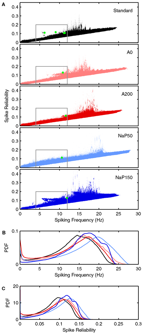
Figure 5. Spiking frequency and spike reliability distribution plots of LM/RAD model variants. (A) Distributions of spiking characteristics (spiking frequency and spike reliability) produced by valid parameter combinations for the Standard, A0, A200, NaP50, and NaP150 variants (top to bottom). The green dots correspond to the average firing behavior exhibited by the specific parameter combinations highlighted in Figures 6 and 7. Regions demarcated in grey correspond to theta-frequency spiking and are shown in greater detail in Figures 8, 10, and 11. (B) Spiking frequency and (C) spike reliability probability density functions (PDFs) for the five variants using the same color scheme as in (A). The PDFs were generated by grouping the spiking frequencies and spike reliabilities into bins of width 0.025 Hz and 0.001 respectively to produce histograms. The histograms were scaled so that the region under each curve is of unit area.

We use the reliability definition and measure given by Schreiber et al. (2003) that involves both spike precision and spike probability because it is appropriate in our context of looking at cholinergic and synaptic inputs to LM/RAD cells. That is, it helps quantify under what (biological, in vivo) conditions the LM/RAD cell fires reliably, since it is a measure of the similarity of responses over trials in which the experimental conditions are fixed (see interpretation in Simulation Procedure). In this way it is analogous to what was done in Schreiber et al. (2009) where they used a constant input with a small oscillatory drive (and added noise). In our case, we have a biological interpretation and context since the changing noise is due to the stochastic synaptic conductances, the constant input is cholinergic, and the oscillatory drive is rhythmicity from the circuit affecting LM/RAD cells. With this interpretation, it is somewhat analogous to considering narrowband (4–12 Hz) rhythmicity except that the spike reliability measure is more tightly coupled to the spiking itself, which is important in our interpretation of the in vivo situation (see Figure 2).

Sensitivity to parameters

For each model variant, the parameter sweep produces two 7-dimensional arrays (one for spiking frequency, S_freq, and one for spike reliability, R_corr) in which each dimension corresponds to a parameter and each index in a dimension corresponds to a particular step value of that parameter. The arrays are not fully populated since certain parameter combinations result in a membrane voltage outside the desired window, and these invalid entries are therefore set to NaN, and not considered.

To investigate the sensitivity of each model variant to the seven different parameters, all the valid entries in the seven-dimensional arrays are grouped in bins of size 0.025 Hz and 0.001 for S_freq and R_corr respectively. For each pair of binned (S_freq, R_corr) values, a list of all the seven-parameter combinations with that (S_freq, R_corr) is generated. Plots of S_freq and R_corr as a function of each parameter are produced by averaging across a given parameter in the list at each (S_freq, R_corr) coordinate. A similar process is used to visualize the membrane voltage, even though it is not treated as a free parameter, by averaging across all voltage values, as given by the V–I curves, associated with each (S_freq, R_corr) pair.

Results

LM/RAD interneurons of the hippocampus express subthreshold theta-frequency (4–12 Hz) MPOs in vitro (Chapman and Lacaille, 1999a), a phenomenon captured by our biophysically based LM/RAD model cell (Morin et al., 2010) as shown in Figure 1A. Our twofold goal is to determine whether these LM/RAD model cells can produce reliable theta-frequency spiking under in vivo-like settings, since this would indicate that they can be important contributors to population theta rhythms, and to determine what conditions would support this. We investigate this computationally by examining a wide spectrum of synaptic background activities and cholinergic levels as well as exploring biophysical dependencies. A sample voltage trace from our LM/RAD model cell under in vivo-like conditions is shown in Figure 1B. Figure 2 is a schematic showing the cell in an in vivo-like network setting, receiving cholinergic input from the medial septum as well as background excitatory and inhibitory synaptic currents.

Isolated (in vitro-like) Behavior of Model Cells

To understand how the biophysical characteristics contribute to spiking behavior in a network environment, it is helpful to first examine the behavior of the isolated model cells, i.e., the model cells in an in vitro-like situation with blocked synapses. The full system of equations representing the LM/RAD model cell (Eq. 1 and Table 1) is 15-dimensional making it challenging to be able to perform mathematical analyses. Thus, as described in Section “Spiking Threshold and Frequency Response of Models,” we perform a numerical analysis to determine the spiking thresholds and frequency responses (f–I curves) of the model variants.

In Figure 3, we show the frequency response of the Standard model variant in the presence (red) and absence (blue) of intrinsic noise. As described in detail in Section “Hippocampal Interneuron Model (‘In vitro’),” the noise is introduced to appropriately characterize the experimental data and is interpreted as stochastic channel gating. The center panel shows the f–I curve, and as expected, spiking can occur at less depolarized values when noise is included in the system (Hô and Destexhe, 2000). The noiseless f–I curve implies that a saddle-node (Type I) bifurcation may be present due to the emergence of spiking at a zero frequency, but more complex dynamics are likely involved since for a small range of injected DC currents, doublet firing is seen before the system exhibits periodic firing at larger DC values. This is illustrated at the top of Figure 3 where three voltage traces are shown for different injected current values in silent, doublet, and regular firing regions. The bottom of Figure 3 shows three voltage waveforms for the system with intrinsic noise. Although the spiking frequencies are similar to the noiseless system, the firing is not perfectly periodic due to the intrinsic noise. As we will see below, the level of intrinsic noise in the model (chosen to appropriately capture the magnitude of experimental MPOs) is superseded by the synaptic “noise” in the in vivo-like scenarios. Overall, it is clear that the Standard model can spike at theta frequencies for a wide range of DC current values.

In Figure 4, we show the frequency responses for the four non-Standard model variants in which the conductances for A-type potassium and persistent sodium currents are modulated (A0, A200, NaP50, NaP150). These particular variants are constructed to have the same conductances as those examined in Morin et al. (2010) to allow for comparison and because these currents were found to be the most important in the generation of MPOs [see Hippocampal Interneuron Model (“In vitro”) and Model Variants]. Reducing (removing) the A-type potassium current (A0 model variant) – Figure 4A – causes a leftward shift in the bifurcation point and a small change in the steepness of the f–I curve relative to the Standard model. However, doublet firing is not seen at lower DC values implying that the bifurcation type may be a saddle-node (Type I). With an increase in the A-type potassium current (A200 model variant) – Figure 4B – besides a rightward shift in the bifurcation point as expected with an increase in an outward current, there now appears to be a Hopf type bifurcation (Type II) with spiking frequencies starting at the high end of the theta range.

A decrease in persistent sodium (NaP50 model variant) – Figure 4C – seems to promote a clear change in its bifurcation type (to Type II, Hopf) since spiking starts at a non-zero value. In addition, this value is at a frequency beyond theta. However, more complex dynamics are probably in play due to the slower currents that delay firing onset (see details in Spiking Threshold and Frequency Response of Models). For the model with a larger persistent sodium current (NaP150 model variant) – Figure 4D – we obtain a shallower increase in frequency with injected current relative to the Standard model so that theta-frequency spiking can occur for a wider range of DC values. Not surprisingly, there is also a leftward shift in its bifurcation point due to the increased amount of inward current in the model. Similar to the Standard model, firing emerges from zero frequency, but unlike the Standard model no doublet firing is observed. This suggests that the NaP150 model may be a Type I oscillator with a saddle-node bifurcation.

Virtual (in vivo-like) Networks

We now turn to an in vivo-like network as schematized in Figure 2. Parameters and values used in the in vivo-like exploration are given in Table 3 and detailed descriptions and rationales are given in Section “Model Parameter Ranges.” All model variants are explored in similarly sized voltage windows that are biased to include their spiking threshold and emphasize fluctuation-driven regimes (see Table 3 and Model Calibration Encompassing and Emphasizing Fluctuation-Driven Regimes). As such, spike reliability comparisons across the five model variants are meaningful and do not contain excessive “outliers” of high reliability (due to very depolarized membrane voltages) or low reliability (due to very hyperpolarized voltages when the cell does not spike).

Given the range and resolution of parameter values in Table 3, there are 430,848,000 possible parameter combinations to consider. The number of valid cases for the five different model variants, with the explicit constraining to the windows of interest as described in Sections “Model Parameter Ranges” and “Simulation Procedure,” are given in Table 4. The fact that the number of valid cases is different for each variant makes sense given the determined window bounds in Table 3 and the fixed resolution used for the parameter values. For example, the number of valid cases is largest for the A200 model variant which has the widest current window bounds.

TABLE 4

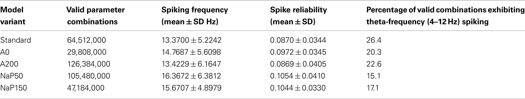
Table 4. Summary of spiking properties for model variants.

Biophysical characteristics and theta spiking reliability

Let us first consider how changing the biophysical characteristics might affect the ability of LM/RAD cells to fire reliably at theta frequencies. For each of the model variants, the average spiking frequency across all valid cases is given in the third column of Table 4. All variants have an average spiking frequency above theta but the Standard variant comes closest to the upper bound of 12 Hz. Note that for some variants, the average in vivo spiking frequency is higher than the spiking frequency given by the f–I curve at the upper limit of the determined window of interest (see Table 3; Figure 4), indicating that fluctuation-driven spiking is indeed a prominent mechanism in our setup. The spike reliability across all valid cases for each model variant is given in the fourth column of Table 4. Except for the A200 variant, the non-Standard model variants have higher average reliabilities. Note that the spike reliability measure we use is dependent on both spike probability and spike precision. Since higher frequencies generally occur further from spike threshold, spike reliability measures would likely be higher for larger frequencies as spike probabilities would be higher. The Standard model variant has the lowest spiking frequency on average so this may also explain why the average reliability for this model appears slightly lower. Finally, if we consider theta-frequency firing as a percentage of valid parameter combinations, as shown in the fifth column of Table 4, we find that the Standard model is the most encompassing of theta-frequency firing, i.e., has the highest percentage. This suggests that the given conductance balances in the Standard model as determined with experimental data (Morin et al., 2010) may reasonably best capture appropriate biological balances.

Figure 5A shows the joint distribution of spike reliabilities and spiking frequencies for the five model variants as described in Section “Sensitivity to Parameters.” In general, there is an upward diagonal shape indicating that higher spike reliabilities occur with higher spiking frequencies as expected. This corroborates our earlier statement regarding the sensitivity of the reliability measure to spiking frequency due to increased spike probability (see Spike Reliability). The regions outlined in gray in Figure 5A delineate theta-frequency firing. As shown by the percentages given in Table 4, the Standard model has the largest fraction of cases in the theta-frequency region relative to the non-Standard variants. Figures 5B,C show the marginal distribution of spiking frequencies and spike reliabilities respectively for the five model variants. It is evident that while the Standard model has on average somewhat lower spike reliabilities relative to the other model variants as given in Table 4 (i.e., left shifted distribution in Figure 5C for the Standard model), firing occurs more readily at theta frequencies (i.e., left shifted distribution in Figure 5B for the Standard model). In other words, the Standard model is best in capturing reliable theta firing.

With the biophysical characteristics of the different LM/RAD model variants, as given by their f–I curves, the distributions shown in Figure 5 make sense. The Standard, A0, and NaP150 model variants, which have Type I-like bifurcations (see Figures 3, and 4A,D), are all able to support reliable firing at lower theta frequencies. This is true for the NaP150 model variant in particular (see Figure 5A – NaP150) which has the least steep f–I curve (see Figure 4D). The A200 and NaP50 model variants which do not have Type I-like bifurcations and intrinsically fire beyond high theta (12 Hz) frequencies (see Figures 4B,C), are less able to support reliable firing at lower theta frequencies (see Figure 5A – A200, NaP50). This is more apparent in the magnified views of the theta-frequency spiking regions presented in Figures 8, 10, and 11. These observations suggest that persistent sodium currents, but not A-type potassium currents, enhance reliable spiking at lower theta frequencies. From our earlier modeling work on subthreshold activities, we note the following: Increasing A-type potassium currents led to a wider and higher neuronal resonant frequency range, whereas increasing persistent sodium currents led to a tighter neuronal resonant frequency range at lower theta frequencies (see Figure 9 in Morin et al., 2010). This therefore suggests that subthreshold, neuronal resonant frequencies can be mirrored in spiking frequencies.

So far, we have discussed reliability measures from a comparative perspective. However, what reliability measure values actually show a clear repeatability across trials at theta frequencies? In Figures 6 and 7, we show examples of reliable theta-frequency spiking for the five model variants, corresponding to the green dots in Figure 5A. Figure 6 depicts four parameter instantiations with similar reliabilities (about 0.1) but different theta spiking frequencies for the Standard variant. On the left side Figures 6A–D are rastergrams of the 20 trials from which the reliability can be gleaned, and on the right are voltage waveforms for two of the trials. Examples from the non-Standard model variants are shown in Figures 7A–D. These examples also have spike reliabilities of about 0.1. The clear repeatability shown in Figures 6 and 7 indicate that a reliability measure value of 0.1 is more than sufficient to conclude that spiking is reliable. For the A200 and NaP50 model variants, there can be large firing gaps. This is presumably due to the non-Type I-like firing of these model cell variants – there is not a gradual onset of spiking frequency from 0 Hz so that jumps between silence and firing can occur for small changes in current drive.

FIGURE 6

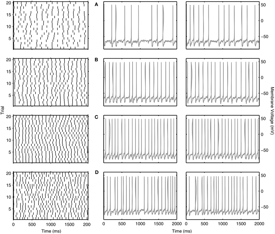
Figure 6. Examples of reliable theta spiking for Standard LM/RAD model. Rastergrams of spiking activity for the 20 trials (left) and sample voltage waveforms for two of the trials (right). Examples shown are indicated as green dots in Figure 5A. Parameter values {I_cholinergic μA/cm², μ_exc mS/cm², μ_inh mS/cm², σ_exc mS/cm², σ_inh mS/cm², A μA/cm², f Hz} and corresponding spiking characteristics {S_freq mean ± SD Hz, R_corr} are: (A) {4.750, 0.04, 0.02, 0.02, 0.10, 0.125, 7} → {6.225 ± 0.678, 0.1105}, (B) {1.375, 0.10, 0.06, 0.02, 0.06, 0.125, 9} → {9.050 ± 0.276, 0.1167}, (C) {1.625, 0.10, 0.06, 0.02, 0.06, 0.100, 8} → {11.175 ± 0.245, 0.1066}, (D) {0.375, 0.16, 0.26, 0.02, 0.03, 0.100, 23} → {11.375 ± 0.741, 0.1077}.

FIGURE 7

Figure 7. Examples of reliable theta spiking for non-Standard LM/RAD model variants. Rastergrams of spiking activity for the 20 trials (left) and sample voltage waveforms for two of the 20 trials (right) for (A) A0, (B) A200, (C) NaP50, and (D) NaP150 model variants. Examples shown are indicated as green dots in Figure 5A. Parameter values {I_cholinergic μA/cm², μ_exc mS/cm², μ_inh mS/cm², σ_exc mS/cm², σ_inh mS/cm², A μA/cm², f Hz} and corresponding spiking characteristics {S_freq mean ± SD Hz, R_corr} are: (A) {2.125, 0.04, 0.02, 0.02, 0.10, 0.125, 11} → {10.875 ± 0.222, 0.1314}, (B) {5.250, 0.10, 0.06, 0.02, 0.06, 0.125, 12} → {11.600 ± 0.754, 0.1140{, (C) {3.625, 0.16, 0.10, 0.02, 0.02, 0.125, 16} → {10.600 ± 1.675, 0.1122}, (D) {3.500, 0.04, 0.02, 0.02, 0.10, 0.075, 12} → {11.875 ± 0.275, 0.1281}.

Overall, our results suggest that Type I oscillator models (Standard, A0, and NaP150 model variants exhibit Type I-like characteristics) are helpful in bringing about reliable theta-frequency firing, and an understanding of the contribution of biophysical characteristics can be garnered by examining f–I curves. However, it is clear that there are more complex dynamics in the system (e.g., see doublet firing of the Standard model in Figure 3 and the complex shape of the reliability-frequency plot of the NaP150 model variant in Figure 5A). We have shown that LM/RAD model cells can produce reliable theta firing in in vivo-like virtual networks, and that this can be somewhat understood from the behavior of the isolated model cells. We now consider which in vivo-like parameter sets are important in bringing about the reliable theta firing.

Fluctuating inhibitory inputs best promote reliable theta spiking

As described in detail in Section “Model Parameter Ranges,” the in vivo-like conditions are chosen around spike threshold values to encompass fluctuation-driven regimes. The seven different parameters that set up the in vivo-like conditions are given in Table 3. The synaptic background activities (conductance means and standard deviations) are chosen to include a wide range of conditions, particularly those that may occur in vivo, such as inhibition-dominated or balanced-conductance states (Piwkowska et al., 2008). In Figures 8 and 11, we show spike reliability and spiking frequency plots for each of the different parameters that set up the in vivo-like state for the Standard model. The plots are color coded for the range of parameter values used and we zoom into the theta-frequency range to better illustrate the impact of individual parameters on reliable theta spiking.

FIGURE 8

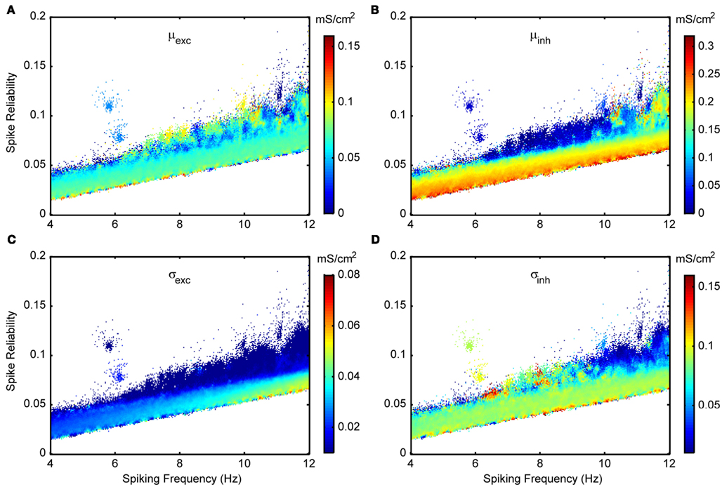
Figure 8. Spike reliability and theta-frequency plots of Standard LM/RAD model for synaptic conductance parameters. Magnified views of the outlined region in Figure 5A showing parameter combinations that produce theta-frequency spiking. The color coding indicates the parameter values as shown on the colorbars for (A) μ_exc – excitatory mean conductance, (B) μ_inh – inhibitory mean conductance, (C) σ_exc – excitatory standard deviation (noise), and (D) σ_inh – inhibitory standard deviation (noise).

Figure 8 shows excitatory and inhibitory conductance mean (Figures 8A,B) and standard deviation (Figures 8C,D) parameters. From the coloring in these plots, we see that there is a wider range of inhibitory parameter values relative to excitatory ones that produce reliable theta firing. To show this more explicitly, we take “frequency slices” of each of the plots in Figure 8 and plot the spike reliability value against the parameter value. This is shown in Figure 9 for a mid-theta-frequency slice of 5.5–7 Hz. From this figure, it is immediately clear that not only are the spike reliability values higher for inhibitory mean (Figure 9A) and standard deviation (Figure 9B) values relative to excitatory values, but also that the range of inhibitory values is much larger. Specifically, whereas we see inhibitory means and standard deviations up to 0.32 and 0.16 mS/cm² respectively (the upper bounds of the ranges explored), we do not see their excitatory counterparts exceed 0.16 and 0.06 mS/cm² (their upper bounds are 0.20 and 0.10 mS/cm²) suggesting that strong excitation precludes reliable mid-theta spiking. Furthermore, from Figure 9B we see that larger inhibitory fluctuations actually enhance reliable firing in the mid-theta range. Specifically, referring back to Figure 8, we see that for spiking frequencies close to 6 Hz, there are patches of higher spike reliability at about 0.06 and 0.11. Given the color coding in Figure 8, and the Figure 9 slice, it is clear that this occurs when high inhibitory fluctuations are present. In summary, from Figures 8 and 9, it is apparent that the production of reliable theta-frequency spiking in model LM/RAD cells (Standard variant) is strongly controlled by inhibitory inputs, and more critically, by inhibitory fluctuations. We also found this to be the case for the other non-Standard model variants, with a larger prevalence of reliable theta firing for high inhibitory fluctuations in the Type I-like oscillator models (A0 and NaP150) relative to the Type II-like oscillator models (A200 and NaP50), especially at low- and mid-theta frequencies. This is shown in Figure 10 where we see that higher inhibitory noise levels can actually prompt the A0 and NaP150 model variants to fire more reliably at low- and mid-theta frequencies. This suggests that Type I-like integrator neurons can be stimulated to fire more reliably by increasing the inhibitory noise level.

FIGURE 9

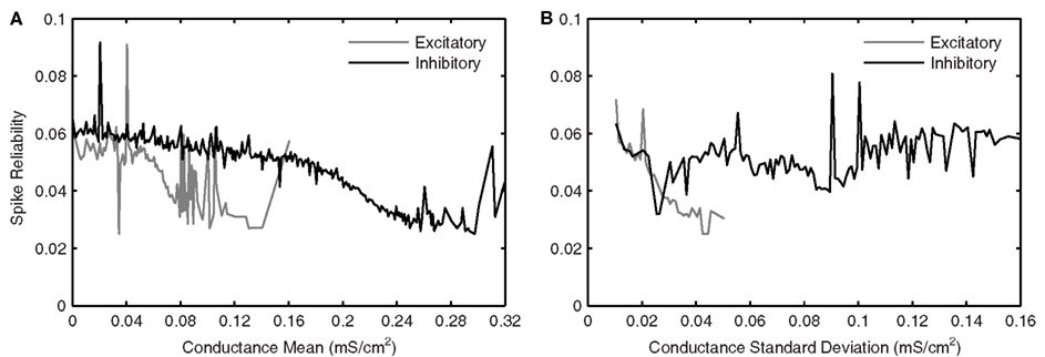
Figure 9. Average effects of synaptic conductance parameters eliciting mid-theta-frequency spiking in Standard LM/RAD model on spike reliability. Average synaptic conductance parameter values eliciting spiking at frequencies between 5.5 and 7 Hz in the Standard model (as given by the color of each coordinate in the 5.5–7 Hz strips in Figure 8) are grouped into bins of width 1 nS/cm². The mean of the reliabilities corresponding to the parameter values in each bin is plotted against binned synaptic conductance (A) means and (B) standard deviations.

FIGURE 10

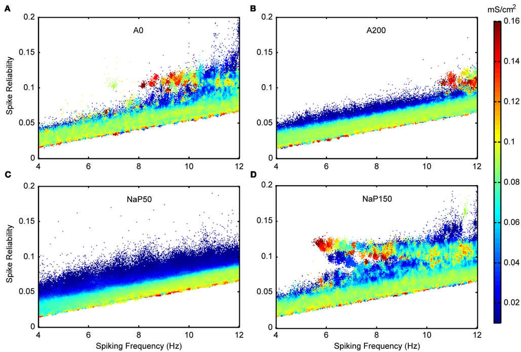
Figure 10. Spike reliability and theta-frequency plots of non-Standard LM/RAD model variants for inhibitory noise parameter. Magnified views of the outlined regions in Figure 5A showing σ_inh – inhibitory standard deviation (noise) – values that produce theta-frequency spiking for (A) A0, (B) A200, (C) NaP50, and (D) NaP150 model variants. Note that for the A0 and NaP150 model variants (Type I-like neurons) there is a non-monotonic relationship between inhibitory noise levels and spike reliability. Indeed, it is clear that for some spiking frequencies, high noise levels are actually required to accomplish higher reliabilities.

Figures 11A, C, D show the other three in vivo-like state parameters examined for the Standard variant. Figure 11B is color coded for the membrane voltage of the model cell, where this value is determined according to the fitted V–I curves if suprathreshold. Note that for each coordinate, the mean conductances (Figures 8A–B), cholinergic current (Figure 11A) and membrane voltage (Figure 11B) are loosely related by Eq. 5. As mentioned in Section “Model Parameter Ranges,” the probe amplitude was intentionally chosen to be small so as to not forcefully pace the neuron and dominate the effect of internal mechanisms. Given the speckled appearance of the plot in Figure 11C, spike reliability and spiking frequency have no clear dependence on the amplitude, at least for the range investigated. It is interesting to note from Figure 11D that although probe frequencies are mainly around 15 Hz and include theta frequencies, higher frequencies in the low gamma/beta frequency range (20–30 Hz) are also included. This suggests that background frequencies of low gamma/beta can be conducive to LM/RAD neurons producing reliable theta-frequency firing. The disjoint patches of high spike reliability can be produced by a wide range of input frequencies (note the speckled appearance of the patches in Figure 11D). Finally, we note that cholinergic inputs seldom exceed about 6 μA/cm² (see Figure 11A) and that depolarized membrane voltages have higher spike reliabilities, and encompass almost the entire range of theta frequencies (see Figure 11B).

FIGURE 11

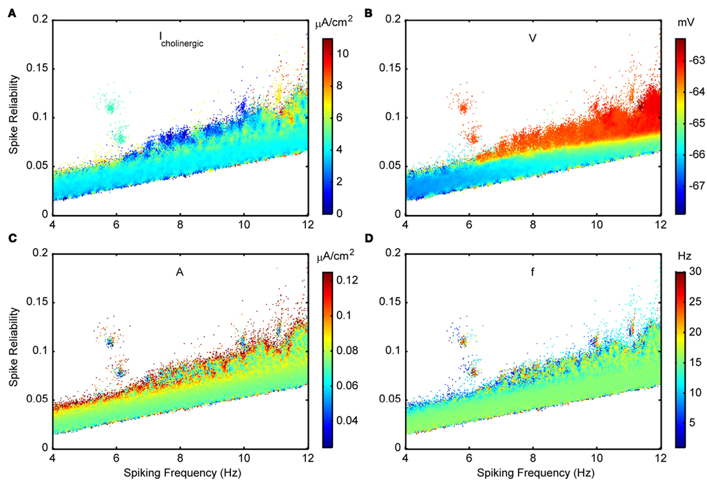
Figure 11. Spike reliability and theta-frequency plots of Standard LM/RAD model for cholinergic and probe parameters. Magnified views of the outlined region in Figure 5A showing parameter combinations that produce theta-frequency spiking. The color coding indicates the parameter values as shown on the colorbars for: (A) I_cholinergic – cholinergic input, (C) A – probe amplitude, and (D) f – probe frequency. (B) Membrane voltage, V, according to the fitted V–I curve.

Given our model results described above, let us consider a potential correspondence with biological LM/RAD cells. Consider the features of the patch of high spike reliability (about 0.1) at around 6 Hz (see Figures 8 and 11). This patch is brought about by a low excitatory noise value of 0.02 mS/cm² but a high inhibitory noise of 0.09 mS/cm², a cholinergic input of about 4 μA/cm², and mean excitatory and inhibitory conductances of about 0.05 mS/cm². Figure 6A shows the rastergram corresponding to a parameter combination with firing properties in the given patch region as indicated by a green dot near (6 Hz, 0.1) in Figure 5A – Standard. Reliable theta spiking is obtained near −63 mV – a couple of millivolts above spike threshold (see Table 3 and Figure 11B). Chapman and Lacaille (1999b) found that the cholinergic agonist carbachol depolarized LM/RAD cells by 1–9 mV resulting in MPOs and spiking activities (Chapman and Lacaille, 1999b). Considering the correspondence between model and experiment, it may be that this is an optimal operating point for LM/RAD cells. Since this operating point is obtained with a cholinergic drive of about 4 μA/cm² in the Standard model, this value may represent a rough estimate of the required level of cholinergic input from the medial septum to LM/RAD neurons to allow them to contribute to population theta rhythms.

Discussion

In this work, we set out to determine whether hippocampal LM/RAD interneurons could spike reliably at theta frequencies (4–12 Hz) under in vivo-like conditions, and thus contribute to population theta rhythms by imposing IPSPs on the pyramidal cell population. Using a previously developed biophysically based single compartment model of LM/RAD cells and applying in vivo-like conditions, we found that clear repeatability exists with spike reliability values of about 0.1. Furthermore, biophysical characteristics of cell models that give rise to Type I-like oscillators (i.e., higher persistent sodium conductances and lower A-type potassium conductances) were better able to support reliable firing at lower theta frequencies.

The in vivo-like conditions included cholinergic inputs, and excitatory and inhibitory synaptic currents. Several points can be made regarding the existence of reliable theta-frequency spiking in LM/RAD model cells: (i) Cholinergic input and mean excitatory conductances rarely exceed 6 μA/cm² and 0.1 mS/cm² respectively, and do not vary much; (ii) inhibitory mean conductance values range widely, encompassing almost the entire range of parameter values explored; (iii) excitatory fluctuations are small, not exceeding 0.04 mS/cm² except for high theta frequencies; (iv) inhibitory fluctuations are large, reaching 0.16 mS/cm² for almost the entire range of theta frequencies; (v) background input (i.e., probe) frequencies include theta suggesting that subthreshold theta-frequency MPOs do manifest in theta spiking frequencies – however, probe frequencies are mainly around 15 Hz and can also include low gamma/beta (20–30 Hz) frequencies; (vi) more depolarized membrane voltages have higher reliabilities, and encompass almost the entire range of theta frequencies.

A major result is the importance of inhibitory inputs in bringing about reliable theta spiking in the LM/RAD model cells. In particular, inhibitory fluctuations greatly exceed excitatory ones. This suggests that inhibitory input to these cells are of critical importance for them to be able to contribute to population theta activities in vivo. This is especially interesting given that other models and dynamic clamp experiments have shown that during high-conductance states or in vivo-like conditions, spikes are mainly determined by inhibitory noise (Destexhe, 2010). Piwkowska et al. (2008) have shown that there is a drop in total synaptic conductance just before spikes are triggered during high-conductance states, and that in inhibition-dominated states, the relationship σ_exc < 0.6σ_inh is satisfied. This is clearly the case for our LM/RAD cells in the high conductance, in vivo-like states. We further note that Hasenstaub et al. (2005) found that inhibition is at least as powerful as excitation in determining spiking probability and timing.

Subthreshold and Suprathreshold Activities

How might subthreshold activities and firing rates be linked? It is known that different cell types display distinct frequency preferences (e.g., Pike et al., 2000; Fellous et al., 2001). The neuronal resonances of different cell types come about because of their biophysical makeup. For example, differences in hyperpolarization-activated inward currents are able to account for much of the resonance differences in hippocampal pyramidal cells and interneurons (Zemankovics et al., 2010). How subthreshold activities are related to firing activities is complicated to understand since it not only depends on the biophysical specifics and mechanisms but also on the network environment (i.e., synaptic activities) that give rise to the firing. Using conductance-based models, Richardson et al. (2003) showed that subthreshold resonance frequencies may or may not be reflected in the firing activities depending on the level of “noise.” In our conductance-based LM/RAD models, we found that theta-frequency subthreshold activities can be reflected in reliable firing activities of similar frequencies for certain balances of “noise” or synaptic activities. However, reliable firing can also be obtained at other frequencies not reflected in the subthreshold activities (see Figure 5). In other words, the network context and cellular character can combine to selectively enhance particular firing frequencies. Therefore, when considering whether subthreshold and suprathreshold activities are linked, the network context and cellular characteristics should be examined together.

Subthreshold oscillations observed in experiment have a noisy appearance and this has been modeled as being either fundamentally deterministic with noise added (Rotstein et al., 2006) or stochastic (Morin et al., 2010) in nature. In particular, Morin et al. considered a critical slowing mechanism in which the subthreshold activity came about due to an enhanced response to (intrinsic) noise. Interestingly, with this critical slowing mechanism, there is an amplitude increase with depolarization approaching threshold as has been observed in both LM/RAD cells (Chapman and Lacaille, 1999a) and stellate cells in the entorhinal cortex (Yoshida et al., 2011). Also, experimental studies using dynamic clamp protocols on stellate cells indicate that intrinsic, channel noise is essential for the presence of subthreshold oscillations (Dorval and White, 2005). Regardless, this subthreshold activity comes about due to the specific biophysical makeup of the cell which in turn influences its firing output (Schreiber et al., 2004). However, using subthreshold activities as a proxy for what output firing could result may or may not be appropriate. For example, the influence of subthreshold oscillations has been suggested to be less important than previously thought since they were found to be significantly attenuated with conductance-based but not current-based inputs (Fernandez and White, 2008). In the approach we took here with consideration of a wide range of in vivo-like network contexts, the subthreshold frequency activities can be reflected in output firing rates when particular network contexts emphasizing inhibitory fluctuations are present.

Limitations and Future Work

Although our model is high-dimensional, it is far from being a complete representation of LM/RAD cells – not only is it a single compartment model, it also does not fully capture certain channel kinetics such as inactivation of the I_D current. We also used a highly simplified intrinsic noise representation (additive) which was assumed to represent stochastic gating, and a minimal representation for cholinergic input. More appropriate stochastic gating models for intrinsic noise can be explored but preliminary studies indicate that subthreshold activities are not significantly affected. Cholinergic control is difficult to examine because of the specificity to cell type (Lawrence et al., 2006). However, similarities between the hippocampus and the neocortex (Lawrence, 2008) imply that a detailed knowledge of these specifics could lead to a general understanding of cholinergic control in brain networks.

It would be interesting to perform detailed mathematical analyses to examine the bifurcation structure of our models. Our work indicated that Type I models (as dictated by the biophysics) might be preferable in bringing about reliable theta firing, but the determination of whether our models were Type I was based on examination of f–I curves and not directly from analyses. Also, Type I models are brought about by saddle-node type bifurcations and do not exhibit subthreshold oscillations. This suggests that subthreshold oscillation generation is stochastic in nature, rather than deterministic. Analyses of our models may help decipher these mechanistic differences and consequences. Another interesting aspect to consider is whether LM/RAD cell networks can exhibit noise-induced synchronization as described in Ermentrout et al. (2008).

Concluding Remarks

The role of noise in the brain has been discussed in the context of spike reliability and synchrony (Ermentrout et al., 2008). Frozen noise inputs generate reliable firing in cortical cells in vitro (e.g., see Mainen and Sejnowski, 1995). That is, there is a similar spike pattern in response to the same fluctuating input. However, determining and examining such patterns (events) in vivo is more challenging because of the more complex environment, but sophisticated techniques are being developed (Tiesinga et al., 2008; Toups et al., 2011). In these studies, reliability is considered to only encompass spike probability, and not both spike probability and spike precision, as with Schreiber et al. (2003, 2009). Overall, these are difficult issues to explore because the nature of the noise matters and could have varied roles in different contexts, depending on what mechanisms may be operating (Wang, 2010). In general, it may not be possible to initially ignore biophysical, cellular details as we need to consider the details to discover the mechanisms and gain understanding in the first place (Skinner, 2012).

Given the diversity of inhibitory cell types and the increasing awareness of the critical role of inhibition (Isaacson and Scanziani, 2011), model studies need to make clear links with experiment. This will allow insights gleaned from modeling to be interpreted in biological settings, and so increase our understanding of the dynamic output of biological networks. The approach we took here was to computationally examine biophysically based models under a wide range of in vivo-like conditions. In this way, we were able to show that subthreshold and suprathreshold activities could be linked for particular network contexts of cholinergic inputs and background synaptic activities, and that inhibitory fluctuations are vital. These particulars are predictive of what balances may exist in vivo. As such, this approach may be a helpful strategy to adopt to untangle what cellular and network interactions may be occurring in brain networks.

Conflict of Interest Statement

The authors declare that the research was conducted in the absence of any commercial or financial relationships that could be construed as a potential conflict of interest.

Acknowledgments

We would like to thank the Natural Sciences and Engineering Research Council (NSERC) of Canada for their support, and Darrell Haufler for help with original model specifics and feedback on the paper. Computations were performed on the GPC supercomputer at the SciNet HPC Consortium. SciNet is funded by: the Canada Foundation for Innovation under the auspices of Compute Canada; the Government of Ontario; Ontario Research Fund – Research Excellence; and the University of Toronto.

References

Bourdeau, M. L., Morin, F., Laurent, C. E., Azzi, M., and Lacaille, J.-C. (2007). Kv4.3-mediated A-type K+ currents underlie rhythmic activity in hippocampal interneurons. J. Neurosci. 27, 1942–1953.

Pubmed Abstract | Pubmed Full Text | CrossRef Full Text

Buzsáki, G. (2002). Theta oscillations in the hippocampus. Neuron 33, 325–340.

Pubmed Abstract | Pubmed Full Text | CrossRef Full Text

Buzsáki, G. (2011). Hippocampus. Scholarpedia J. 6, 1468.

CrossRef Full Text

Buzsáki, G., and Draguhn, A. (2004). Neuronal oscillations in cortical networks. Science 304, 1926–1929.

Pubmed Abstract | Pubmed Full Text | CrossRef Full Text

Chapman, C. A., and Lacaille, J.-C. (1999a). Intrinsic theta-frequency membrane potential oscillations in hippocampal CA1 interneurons of stratum lacunosum-moleculare. J. Neurophysiol. 81, 1296–1307.

Chapman, C. A., and Lacaille, J.-C. (1999b). Cholinergic induction of theta-frequency oscillations in hippocampal inhibitory interneurons and pacing of pyramidal cell firing. J. Neurosci. 19, 8637–8645.

Destexhe, A. (2007). High-conductance state. Scholarpedia J. 2, 1341.

CrossRef Full Text

Destexhe, A. (2010). Inhibitory “noise”. Front. Cell. Neurosci. 4:9. doi:10.3389/fncel.2010.00009

CrossRef Full Text

Destexhe, A., Rudolph, M., Fellous, J.-M., and Sejnowski, T. J. (2001). Fluctuating synaptic conductances recreate in vivo-like activity in neocortical neurons. Neuroscience 107, 13–24.

Pubmed Abstract | Pubmed Full Text | CrossRef Full Text

Destexhe, A., Rudolph, M., and Paré, D. (2003). The high-conductance state of neocortical neurons in vivo. Nat. Rev. Neurosci. 4, 739–751.

Pubmed Abstract | Pubmed Full Text | CrossRef Full Text

Dorval, A. D. Jr., and White, J. A. (2005). Channel noise is essential for perithreshold oscillations in entorhinal stellate neurons. J. Neurosci. 25, 10025–10028.

Pubmed Abstract | Pubmed Full Text | CrossRef Full Text

Ermentrout, G. B., Galán, R. F., and Urban, N. N. (2008). Reliability, synchrony and noise. Trends Neurosci. 31, 428–434.

Pubmed Abstract | Pubmed Full Text | CrossRef Full Text

Fellous, J.-M., Houweling, A. R., Modi, R. H., Rao, R. P., Tiesinga, P. H., and Sejnowski, T. J. (2001). Frequency dependence of spike timing reliability in cortical pyramidal cells and interneurons. J. Neurophysiol. 85, 1782–1787.

Pubmed Abstract | Pubmed Full Text

Fernandez, F. R., and White, J. A. (2008). Artificial synaptic conductances reduce subthreshold oscillations and periodic firing in stellate cells of the entorhinal cortex. J. Neurosci. 28, 3790–3803.

Pubmed Abstract | Pubmed Full Text | CrossRef Full Text

Hasenstaub, A., Shu, Y., Haider, B., Kraushaar, U., Duque, A., and McCormick, D. A. (2005). Inhibitory postsynaptic potentials carry synchronized frequency information in active cortical networks. Neuron 47, 423–435.

Pubmed Abstract | Pubmed Full Text | CrossRef Full Text

Hô, N., and Destexhe, A. (2000). Synaptic background activity enhances the responsiveness of neocortical pyramidal neurons. J. Neurophysiol. 84, 1488–1496.

Pubmed Abstract | Pubmed Full Text

Isaacson, J. S., and Scanziani, M. (2011). How inhibition shapes cortical activity. Neuron 72, 231–243.

Pubmed Abstract | Pubmed Full Text | CrossRef Full Text

Klausberger, T., and Somogyi, P. (2008). Neuronal diversity and temporal dynamics: The unity of hippocampal circuit operations. Science 321, 53–57.

Pubmed Abstract | Pubmed Full Text | CrossRef Full Text

Lawrence, J. J. (2008). Cholinergic control of GABA release: emerging parallels between neocortex and hippocampus. Trends Neurosci. 31, 317–327.

Pubmed Abstract | Pubmed Full Text | CrossRef Full Text

Lawrence, J. J., Statland, J. M., Grinspan, Z. M., and McBain, C. J. (2006). Cell type-specific dependence of muscarinic signalling in mouse hippocampal stratum oriens interneurons. J. Physiol. (Lond.) 570, 595–610.

Pubmed Abstract | Pubmed Full Text | CrossRef Full Text

Loken, C., Gruner, D., Groer, L., Peltier, R., Bunn, N., Craig, M., Henriques, T., Dempsey, J., Yu, C.-H., Chen, J., Dursi, J. L., Chong, J., Northrup, S., Pinto, J., Knecht, N., and Van Zon, R. (2010). SciNet: lessons learned from building a power-efficient top-20 system and data centre. J. Phys. Conf. Ser. 256, 2–36.

CrossRef Full Text

Mainen, Z. F., and Sejnowski, T. J. (1995). Reliability of spike timing in neocortical neurons. Science 268, 1503–1506.

Pubmed Abstract | Pubmed Full Text | CrossRef Full Text

Morin, F., Haufler, D., Skinner, F. K., and Lacaille, J.-C. (2010). Characterization of voltage-gated K+ currents contributing to subthreshold membrane potential oscillations in hippocampal CA1 interneurons. J. Neurophysiol. 103, 3472–3489.

Pubmed Abstract | Pubmed Full Text | CrossRef Full Text

Pike, F. G., Goddard, R. S., Suckling, J. M., Ganter, P., Kasthuri, N., and Paulsen, O. (2000). Distinct frequency preferences of different types of rat hippocampal neurons in response to oscillatory input currents. J. Physiol. (Lond.) 529, 205–213.

Pubmed Abstract | Pubmed Full Text | CrossRef Full Text

Piwkowska, Z., Pospischil, M., Brette, R., Sliwa, J., Rudolph-Lilith, M., Bal, T., and Destexhe, A. (2008). Characterizing synaptic conductance fluctuations in cortical neurons and their influence on spike generation. J. Neurosci. Methods 169, 302–322.

Pubmed Abstract | Pubmed Full Text | CrossRef Full Text

Richardson, M. J. E., Brunel, N., and Hakim, V. (2003). From subthreshold to firing-rate resonance. J. Neurophysiol. 89, 2538–2554.

Pubmed Abstract | Pubmed Full Text | CrossRef Full Text

Rotstein, H. G., Oppermann, T., White, J. A., and Kopell, N. (2006). The dynamic structure underlying subthreshold oscillatory activity and the onset of spikes in a model of medial entorhinal cortex stellate cells. J. Comput. Neurosci. 21, 271–292.

Pubmed Abstract | Pubmed Full Text | CrossRef Full Text

Schreiber, S., Fellous, J.-M., Tiesinga, P., and Sejnowski, T. J. (2004). Influence of ionic conductances on spike timing reliability of cortical neurons for suprathreshold rhythmic inputs. J. Neurophysiol. 91, 194–205.

Pubmed Abstract | Pubmed Full Text | CrossRef Full Text

Schreiber, S., Fellous, J.-M., Whitmer, D., Tiesinga, P., and Sejnowski, T. J. (2003). A new correlation-based measure of spike timing reliability. Neurocomputing 52–54, 925–931.

Pubmed Abstract | Pubmed Full Text | CrossRef Full Text

Schreiber, S., Samengo, I., and Herz, A. V. M. (2009). Two distinct mechanisms shape the reliability of neural responses. J. Neurophysiol. 101, 2239–2251.

Pubmed Abstract | Pubmed Full Text | CrossRef Full Text

Skinner, F. K. (2012). Cellular-based modeling of oscillatory dynamics in brain networks. Curr. Opin. Neurobiol. 22. doi:10.1016/j.conb.2012.02.00. [Epub ahead of print].

CrossRef Full Text

Steyn-Ross, D. A., Steyn-Ross, M. L., Wilson, M. T., and Sleigh, J. W. (2006). White-noise susceptibility and critical slowing in neurons near spiking threshold. Phys. Rev. E Stat. Nonlin. Soft Matter Phys. 74(Pt 1), 051920.

Pubmed Abstract | Pubmed Full Text | CrossRef Full Text

Tiesinga, P., Fellous, J.-M., and Sejnowski, T. J. (2008). Regulation of spike timing in visual cortical circuits. Nat. Rev. Neurosci. 9, 97–107.

Pubmed Abstract | Pubmed Full Text | CrossRef Full Text

Toups, J. V., Fellous, J.-M., Thomas, P. J., Sejnowski, T. J., and Tiesinga, P. H. (2011). Finding the event structure of neuronal spike trains. Neural. Comput. 23, 2169–2208.

Pubmed Abstract | Pubmed Full Text | CrossRef Full Text

Vida, I. (2010). “Morphology of hippocampal neurons,” in Hippocampal Microcircuits: A Computational Modeler’s Resource Book, eds. V. Cutsuridis, B. Graham, S. Cobb, and I. Vida (New York: Springer), 27–68.

Wang, X.-J. (2010). Neurophysiological and computational principles of cortical rhythms in cognition. Physiol. Rev. 90, 1195–1268.

Pubmed Abstract | Pubmed Full Text | CrossRef Full Text

Williams, S., Samulack, D. D., Beaulieu, C., and Lacaille, J. C. (1994). Membrane properties and synaptic responses of interneurons located near the stratum lacunosum-moleculare/radiatum border of area CA1 in whole-cell recordings from rat hippocampal slices. J. Neurophysiol. 71, 2217–2235.

Pubmed Abstract | Pubmed Full Text

Yoshida, M., Giocomo, L. M., Boardman, I., and Hasselmo, M. E. (2011). Frequency of subthreshold oscillations at different membrane potential voltages in neurons at different anatomical positions on the dorsoventral axis in the rat medial entorhinal cortex. J. Neurosci. 31, 12683–12694.

Pubmed Abstract | Pubmed Full Text | CrossRef Full Text

Zemankovics, R., Káli, S., Paulsen, O., Freund, T. F., and Hájos, N. (2010). Differences in subthreshold resonance of hippocampal pyramidal cells and interneurons: the role of h-current and passive membrane characteristics. J. Physiol. (Lond.) 588, 2109–2132.

Pubmed Abstract | Pubmed Full Text | CrossRef Full Text