Invariant visual object and face recognition: neural and computational bases, and a model, VisNet

1. Introduction

One of the major problems that is solved by the visual system in the cerebral cortex is the building of a representation of visual information which allows object and face recognition to occur relatively independently of size, contrast, spatial-frequency, position on the retina, angle of view, lighting, etc. These invariant representations of objects, provided by the inferior temporal visual cortex (Rolls, 2008b), are extremely important for the operation of many other systems in the brain, for if there is an invariant representation, it is possible to learn on a single trial about reward/punishment associations of the object, the place where that object is located, and whether the object has been seen recently, and then to correctly generalize to other views, etc. of the same object (Rolls, 2008b). The way in which these invariant representations of objects are formed is a major issue in understanding brain function, for with this type of learning, we must not only store and retrieve information, but we must solve in addition the major computational problem of how all the different images on the retina (position, size, view, etc.) of an object can be mapped to the same representation of that object in the brain. It is this process with which we are concerned in this paper.

In Section 2 of this paper, I summarize some of the evidence on the nature of the invariant representations of objects and faces found in the inferior temporal visual cortex as shown by neuronal recordings. A fuller account is provided in Memory, Attention, and Decision-Making, Chapter 4 (Rolls, 2008b). Then I build on that foundation a closely linked computational theory of how these invariant representations of objects and faces may be formed by self-organizing learning in the brain, which has been investigated by simulations in a model network, VisNet (Rolls, 1992, 2008b; Wallis and Rolls, 1997; Rolls and Milward, 2000).

This paper reviews this combined neurophysiological and computational neuroscience approach developed by the author which leads to a theory of invariant visual object recognition, and relates this approach to other research.

2. Invariant Representations of Faces and Objects in the Inferior Temporal Visual Cortex

2.1. Processing to the Inferior Temporal Cortex in the Primate Visual System

A schematic diagram to indicate some aspects of the processing involved in object identification from the primary visual cortex, V1, through V2 and V4 to the posterior inferior temporal cortex (TEO) and the anterior inferior temporal cortex (TE) is shown in Figure 1 (Rolls and Deco, 2002; Rolls, 2008b; Blumberg and Kreiman, 2010; Orban, 2011). The approximate location of these visual cortical areas on the brain of a macaque monkey is shown in Figure 2, which also shows that TE has a number of different subdivisions. The different TE areas all contain visually responsive neurons, as do many of the areas within the cortex in the superior temporal sulcus (Baylis et al., 1987). For the purposes of this summary, these areas will be grouped together as the anterior inferior temporal cortex (IT), except where otherwise stated.

FIGURE 1

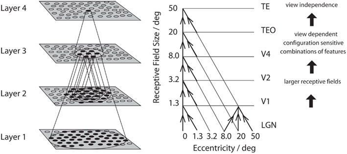
Figure 1. Convergence in the visual system. Right – as it occurs in the brain. V1, visual cortex area V1; TEO, posterior inferior temporal cortex; TE, inferior temporal cortex (IT). Left – as implemented in VisNet. Convergence through the network is designed to provide fourth layer neurons with information from across the entire input retina.

FIGURE 2

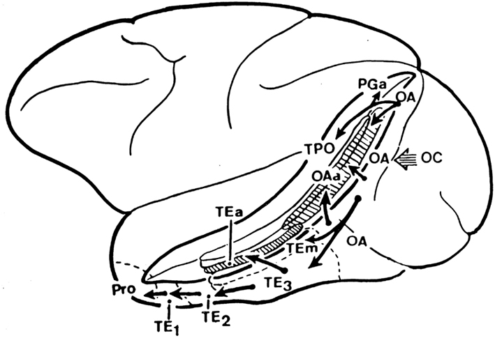
Figure 2. Lateral view of the macaque brain (left hemisphere) showing the different architectonic areas (e.g., TEm, TEa) in and bordering the anterior part of the superior temporal sulcus (STS) of the macaque (see text). The STS has been drawn opened to reveal the cortical areas inside it, and is circumscribed by a thick line.

The object and face-selective neurons described in this paper are found mainly between 7 and 3 mm posterior to the sphenoid reference, which in a 3–4 kg macaque corresponds to approximately 11–15 mm anterior to the interaural plane (Baylis et al., 1987; Rolls, 2007a,b, 2008b). For comparison, the “middle face patch” of Tsao et al. (2006) was at A6, which is probably part of the posterior inferior temporal cortex (Tsao and Livingstone, 2008). In the anterior inferior temporal cortex areas we have investigated, there are separate regions specialized for face identity in areas TEa and TEm on the ventral lip of the superior temporal sulcus and the adjacent gyrus, for face expression and movement in the cortex deep in the superior temporal sulcus (Baylis et al., 1987; Hasselmo et al., 1989a; Rolls, 2007b), and separate neuronal clusters for objects (Booth and Rolls, 1998; Kriegeskorte et al., 2008; Rolls, 2008b). A possible way in which VisNet could produce separate representations of face identity and expression has been investigated (Tromans et al., 2011). Similarly, in humans there are a number of separate visual representations of faces and other body parts (Spiridon et al., 2006; Weiner and Grill-Spector, 2011), with the clustering together of neurons with similar responses influenced by the self-organizing map processes that are a result of cortical design (Rolls, 2008b).

2.2. Translation Invariance and Receptive Field Size

There is convergence from each small part of a region to the succeeding region (or layer in the hierarchy) in such a way that the receptive field sizes of neurons (for example, 1° near the fovea in V1) become larger by a factor of approximately 2.5 with each succeeding stage. (The typical parafoveal receptive field sizes found would not be inconsistent with the calculated approximations of, for example, 8° in V4, 20° in TEO, and 50° in inferior temporal cortex Boussaoud et al., 1991; see Figure 1). Such zones of convergence would overlap continuously with each other (see Figure 1). This connectivity provides part of the basis for the fact that many neurons in the temporal cortical visual areas respond to a stimulus relatively independently of where it is in their receptive field, and moreover maintain their stimulus selectivity when the stimulus appears in different parts of the visual field (Gross et al., 1985; Tovee et al., 1994; Rolls et al., 2003). This is called translation or shift invariance. In addition to having topologically appropriate connections, it is necessary for the connections to have the appropriate synaptic weights to perform the mapping of each set of features, or object, to the same set of neurons in IT. How this could be achieved is addressed in the computational neuroscience models described later in this paper.

2.3. Reduced Translation Invariance in Natural Scenes, and the Selection of a Rewarded Object

Until recently, research on translation invariance considered the case in which there is only one object in the visual field. What happens in a cluttered, natural, environment? Do all objects that can activate an inferior temporal neuron do so whenever they are anywhere within the large receptive fields of inferior temporal neurons (Sato, 1989; Rolls and Tovee, 1995a)? If so, the output of the visual system might be confusing for structures that receive inputs from the temporal cortical visual areas. If one of the objects in the visual field was associated with reward, and another with punishment, would the output of the inferior temporal visual cortex to emotion-related brain systems be an amalgam of both stimuli? If so, how would we be able to choose between the stimuli, and have an emotional response to one but not perhaps the other, and select one for action and not the other (see Figure 3).

FIGURE 3

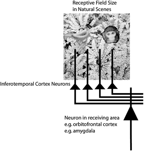
Figure 3. Objects shown in a natural scene, in which the task was to search for and touch one of the stimuli. The objects in the task as run were smaller. The diagram shows that if the receptive fields of inferior temporal cortex neurons are large in natural scenes with multiple objects (in this scene, bananas, and a face), then any receiving neuron in structures such as the orbitofrontal cortex and amygdala would receive information from many stimuli in the field of view, and would not be able to provide evidence about each of the stimuli separately.

To investigate how information is passed from the inferior temporal cortex (IT) to other brain regions to enable stimuli to be selected from natural scenes for action, Rolls et al. (2003) analyzed the responses of single and simultaneously recorded IT neurons to stimuli presented in complex natural backgrounds. In one situation, a visual fixation task was performed in which the monkey fixated at different distances from the effective stimulus. In another situation the monkey had to search for two objects on a screen, and a touch of one object was rewarded with juice, and of another object was punished with saline (see Figure 3 for a schematic overview and Figure 30 for the actual display). In both situations neuronal responses to the effective stimuli for the neurons were compared when the objects were presented in the natural scene or on a plain background. It was found that the overall response of the neuron to objects was sometimes somewhat reduced when they were presented in natural scenes, though the selectivity of the neurons remained. However, the main finding was that the magnitudes of the responses of the neurons typically became much less in the real scene the further the monkey fixated in the scene away from the object (see Figures 4 and 31 and Section 5.8.1).

FIGURE 4

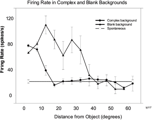
Figure 4. Firing of a temporal cortex cell to an effective stimulus presented either in a blank background or in a natural scene, as a function of the angle in degrees at which the monkey was fixating away from the effective stimulus. The task was to search for and touch the stimulus. (After Rolls et al., 2003.)

It is proposed that this reduced translation invariance in natural scenes helps an unambiguous representation of an object which may be the target for action to be passed to the brain regions that receive from the primate inferior temporal visual cortex. It helps with the binding problem, by reducing in natural scenes the effective receptive field of inferior temporal cortex neurons to approximately the size of an object in the scene. The computational utility and basis for this is considered in Section 5.8 and by Rolls and Deco (2002), Trappenberg et al. (2002), Deco and Rolls (2004), Aggelopoulos and Rolls (2005), and Rolls and Deco (2006), and includes an advantage for what is at the fovea because of the large cortical magnification of the fovea, and shunting interactions between representations weighted by how far they are from the fovea.

These findings suggest that the principle of providing strong weight to whatever is close to the fovea is an important principle governing the operation of the inferior temporal visual cortex, and in general of the output of the ventral visual system in natural environments. This principle of operation is very important in interfacing the visual system to action systems, because the effective stimulus in making inferior temporal cortex neurons fire is in natural scenes usually on or close to the fovea. This means that the spatial coordinates of where the object is in the scene do not have to be represented in the inferior temporal visual cortex, nor passed from it to the action selection system, as the latter can assume that the object making IT neurons fire is close to the fovea in natural scenes. Thus the position in visual space being fixated provides part of the interface between sensory representations of objects and their coordinates as targets for actions in the world. The small receptive fields of IT neurons in natural scenes make this possible. After this, local, egocentric, processing implemented in the dorsal visual processing stream using, e.g., stereodisparity may be used to guide action toward objects being fixated (Rolls and Deco, 2002).

The reduced receptive field size in complex natural scenes also enables emotions to be selective to just what is being fixated, because this is the information that is transmitted by the firing of IT neurons to structures such as the orbitofrontal cortex and amygdala.

There is an important comparison to be made here with some approaches in engineering in which attempts are made to analyze a whole visual scene at once. This is a massive computational problem, not yet solved in engineering. It is very instructive to see that this is not the approach taken by the (primate and human) brain, which instead analyses in complex natural scenes what is close to the fovea, just massively reducing the computational including feature binding problems. The brain then deals with a complex scene by fixating different parts serially, using processes such as bottom-up saliency to guide where fixations should occur (Itti and Koch, 2000; Zhao and Koch, 2011).

Interestingly, although the size of the receptive fields of inferior temporal cortex neurons becomes reduced in natural scenes so that neurons in IT respond primarily to the object being fixated, there is nevertheless frequently some asymmetry in the receptive fields (see Section 5.9 and Figure 35). This provides a partial solution to how multiple objects and their positions in a scene can be captured with a single glance (Aggelopoulos and Rolls, 2005).

2.4. Size and Spatial-Frequency Invariance

Some neurons in the inferior temporal visual cortex and cortex in the anterior part of the superior temporal sulcus (IT/STS) respond relatively independently of the size of an effective face stimulus, with a mean size-invariance (to a half maximal response) of 12 times (3.5 octaves; Rolls and Baylis, 1986). An example of the responses of an inferior temporal cortex face-selective neuron to faces of different sizes is shown in Figure 5. This is not a property of a simple single-layer network (see Figure 7), nor of neurons in V1, which respond best to small stimuli, with a typical size-invariance of 1.5 octaves. Also, the neurons typically responded to a face when the information in it had been reduced from 3D to a 2D representation in gray on a monitor, with a response that was on average 0.5 of that to a real face.

FIGURE 5

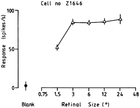
Figure 5. Typical response of an inferior temporal cortex face-selective neuron to faces of different sizes. The size subtended at the retina in degrees is shown. (From Rolls and Baylis, 1986.)

Another transform over which recognition is relatively invariant is spatial-frequency. For example, a face can be identified when it is blurred (when it contains only low-spatial frequencies), and when it is high-pass spatial-frequency filtered (when it looks like a line drawing). If the face images to which these neurons respond are low-pass filtered in the spatial-frequency domain (so that they are blurred), then many of the neurons still respond when the images contain frequencies only up to 8 cycles per face. Similarly, the neurons still respond to high-pass filtered images (with only high-spatial-frequency edge information) when frequencies down to only 8 cycles per face are included (Rolls et al., 1985). Face recognition shows similar invariance with respect to spatial-frequency (see Rolls et al., 1985). Further analysis of these neurons with narrow (octave) bandpass spatial-frequency filtered face stimuli shows that the responses of these neurons to an unfiltered face can not be predicted from a linear combination of their responses to the narrow bandstimuli (Rolls et al., 1987). This lack of linearity of these neurons, and their responsiveness to a wide range of spatial frequencies (see also their broad critical bandmasking Rolls, 2008a), indicate that in at least this part of the primate visual system recognition does not occur using Fourier analysis of the spatial-frequency components of images.

The utility of this representation for memory systems in the brain is that the output of the visual system will represent an object invariantly with respect to position on the retina, size, etc. and this simplifies the functionality required of the (multiple) memory systems, which need then simply associate the object representation with reward (orbitofrontal cortex and amygdala), associate it with position in the environment (hippocampus), recognize it as familiar (perirhinal cortex), associate it with a motor response in a habit memory (basal ganglia), etc. (Rolls, 2008b). The associations can be relatively simple, involving, for example, Hebbian associativity (Rolls, 2008b).

Some neurons in the temporal cortical visual areas actually represent the absolute size of objects such as faces independently of viewing distance (Rolls and Baylis, 1986). This could be called neurophysiological size constancy. The utility of this representation by a small population of neurons is that the absolute size of an object is a useful feature to use as an input to neurons that perform object recognition. Faces only come in certain sizes.

2.5. Combinations of Features in the Correct Spatial Configuration

Many neurons in this ventral processing stream respond to combinations of features (including objects), but not to single features presented alone, and the features must have the correct spatial arrangement. This has been shown, for example, with faces, for which it has been shown by masking out or presenting parts of the face (for example, eyes, mouth, or hair) in isolation, or by jumbling the features in faces, that some cells in the cortex in IT/STS respond only if two or more features are present, and are in the correct spatial arrangement (Perrett et al., 1982; Rolls et al., 1994; Freiwald et al., 2009; Rolls, 2011b). Figure 6 shows examples of four neurons, the top one of which responds only if all the features are present, and the others of which respond not only to the full-face, but also to one or more features. Corresponding evidence has been found for non-face cells. For example Tanaka et al. (1990) showed that some posterior inferior temporal cortex neurons might only respond to the combination of an edge and a small circle if they were in the correct spatial relationship to each other. Consistent evidence for face part configuration sensitivity has been found in human fMRI studies (Liu et al., 2010).

FIGURE 6

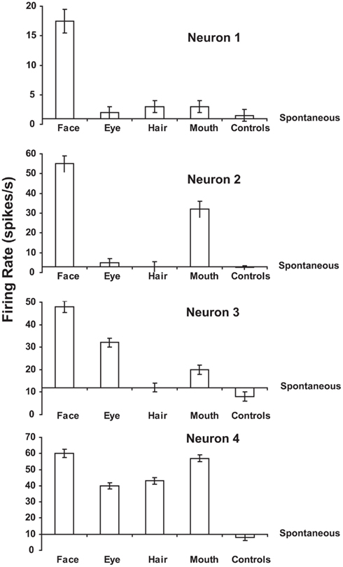
Figure 6. Responses of four temporal cortex neurons to whole faces and to parts of faces. The mean firing rate ± sem are shown. The responses are shown as changes from the spontaneous firing rate of each neuron. Some neurons respond to one or several parts of faces presented alone. Other neurons (of which the top one is an example) respond only to the combination of the parts (and only if they are in the correct spatial configuration with respect to each other as shown by Rolls et al., 1994). The control stimuli were non-face objects. (After Perrett et al., 1982.)

These findings are important for the computational theory, for they show that neurons selective to feature combinations are part of the process by which the cortical hierarchy operates, and this is incorporated into VisNet (Elliffe et al., 2002).

Evidence consistent with the suggestion that neurons are responding to combinations of a few variables represented at the preceding stage of cortical processing is that some neurons in V2 and V4 respond to end-stopped lines, to tongues flanked by inhibitory subregions, to combinations of lines, to combinations of colors, or to surfaces (Hegde and Van Essen, 2000, 2003, 2007; Ito and Komatsu, 2004; Brincat and Connor, 2006; Anzai et al., 2007; Orban, 2011). In the inferior temporal visual cortex, some neurons respond to spatial configurations of surface fragments to help specify the three-dimensional structure of objects (Yamane et al., 2008).

2.6. A View-Invariant Representation

For recognizing and learning about objects (including faces), it is important that an output of the visual system should be not only translation and size invariant, but also relatively view-invariant. In an investigation of whether there are such neurons, we found that some temporal cortical neurons reliably responded differently to the faces of two different individuals independently of viewing angle (Hasselmo et al., 1989b), although in most cases (16/18 neurons) the response was not perfectly view-independent. Mixed together in the same cortical regions there are neurons with view-dependent responses (for example, Hasselmo et al., 1989b; Rolls and Tovee, 1995b). Such neurons might respond, for example, to a view of a profile of a monkey but not to a full-face view of the same monkey (Perrett et al., 1985; Hasselmo et al., 1989b).

These findings of view-dependent, partially view-independent, and view-independent representations in the same cortical regions are consistent with the hypothesis discussed below that view-independent representations are being built in these regions by associating together the outputs of neurons that have different view-dependent responses to the same individual. These findings also provide evidence that one output of the visual system includes representations of what is being seen, in a view-independent way that would be useful for object recognition and for learning associations about objects; and that another output is a view-based representation that would be useful in social interactions to determine whether another individual is looking at one, and for selecting details of motor responses, for which the orientation of the object with respect to the viewer is required (Rolls, 2008b).

Further evidence that some neurons in the temporal cortical visual areas have object-based rather than view-based responses comes from a study of a population of neurons that responds to moving faces (Hasselmo et al., 1989b). For example, four neurons responded vigorously to a head undergoing ventral flexion, irrespective of whether the view of the head was full-face, of either profile, or even of the back of the head. These different views could only be specified as equivalent in object-based coordinates. Further, the movement specificity was maintained across inversion, with neurons responding, for example, to ventral flexion of the head irrespective of whether the head was upright or inverted. In this procedure, retinally encoded or viewer-centered movement vectors are reversed, but the object-based description remains the same.

Also consistent with object-based encoding is the finding of a small number of neurons that respond to images of faces of a given absolute size, irrespective of the retinal image size, or distance (Rolls and Baylis, 1986).

Neurons with view-invariant responses to objects seen naturally by macaques have also been described (Booth and Rolls, 1998). The stimuli were presented for 0.5 s on a color video monitor while the monkey performed a visual fixation task. The stimuli were images of 10 real plastic objects that had been in the monkey’s cage for several weeks, to enable him to build view-invariant representations of the objects. Control stimuli were views of objects that had never been seen as real objects. The neurons analyzed were in the TE cortex in and close to the ventral lip of the anterior part of the superior temporal sulcus. Many neurons were found that responded to some views of some objects. However, for a smaller number of neurons, the responses occurred only to a subset of the objects (using ensemble encoding), irrespective of the viewing angle. Moreover, the firing of a neuron on any one trial, taken at random and irrespective of the particular view of any one object, provided information about which object had been seen, and this information increased approximately linearly with the number of neurons in the sample. This is strong quantitative evidence that some neurons in the inferior temporal cortex provide an invariant representation of objects. Moreover, the results of Booth and Rolls (1998) show that the information is available in the firing rates, and has all the desirable properties of distributed representations, including exponentially high-coding capacity, and rapid speed of read-out of the information (Rolls, 2008b; Rolls and Treves, 2011).

Further evidence consistent with these findings is that some studies have shown that the responses of some visual neurons in the inferior temporal cortex do not depend on the presence or absence of critical features for maximal activation (Perrett et al., 1982; Tanaka, 1993, 1996). For example, neuron 4 in Figure 6 responded to several of the features in a face when these features were presented alone (Perrett et al., 1982). In another example, Mikami et al. (1994) showed that some TE cells respond to partial views of the same laboratory instrument(s), even when these partial views contain different features. Such functionality is important for object recognition when part of an object is occluded, by, for example, another object. In a different approach, Logothetis et al. (1994) have reported that in monkeys extensively trained (over thousands of trials) to treat different views of computer generated wire-frame “objects” as the same, a small population of neurons in the inferior temporal cortex did respond to different views of the same wire-frame object (see also Logothetis and Sheinberg, 1996). However, extensive training is not necessary for invariant representations to be formed, and indeed no explicit training in invariant object recognition was given in the experiment by Booth and Rolls (1998), as Rolls’ hypothesis (Rolls, 1992) is that view-invariant representations can be learned by associating together the different views of objects as they are moved and inspected naturally in a period that may be in the order of a few seconds. Evidence for this is described in Section 2.7.

2.7. Learning of New Representations in the Temporal Cortical Visual Areas

To investigate the idea that visual experience might guide the formation of the responsiveness of neurons so that they provide an economical and ensemble-encoded representation of items actually present in the environment (and indeed any rapid learning found might help in the formation of invariant representations), the responses of inferior temporal cortex face-selective neurons have been analyzed while a set of new faces were shown. Some of the neurons studied in this way altered the relative degree to which they responded to the different members of the set of novel faces over the first few (1–2) presentations of the set (Rolls et al., 1989). If in a different experiment a single novel face was introduced when the responses of a neuron to a set of familiar faces were being recorded, the responses to the set of familiar faces were not disrupted, while the responses to the novel face became stable within a few presentations. Alteration of the tuning of individual neurons in this way may result in a good discrimination over the population as a whole of the faces known to the monkey. This evidence is consistent with the categorization being performed by self-organizing competitive neuronal networks, as described elsewhere (Rolls and Treves, 1998; Rolls, 2008b). Further evidence has been found to support the hypothesis (Rolls, 1992, 2008b) that unsupervised natural experience rapidly alters invariant object representation in the visual cortex (Li and DiCarlo, 2008; Li et al., 2011; cf. Folstein et al., 2010).

Further evidence that these neurons can learn new representations very rapidly comes from an experiment in which binarized black and white (two-tone) images of faces that blended with the background were used. These did not activate face-selective neurons. Full gray-scale images of the same photographs were then shown for ten 0.5 s presentations. In a number of cases, if the neuron happened to be responsive to that face, when the binarized version of the same face was shown next, the neurons responded to it (Tovee et al., 1996). This is a direct parallel to the same phenomenon that is observed psychophysically, and provides dramatic evidence that these neurons are influenced by only a very few seconds (in this case 5 s) of experience with a visual stimulus. We have shown a neural correlate of this effect using similar stimuli and a similar paradigm in a PET (positron emission tomography) neuroimaging study in humans, with a region showing an effect of the learning found for faces in the right temporal lobe, and for objects in the left temporal lobe (Dolan et al., 1997).

Once invariant representations of objects have been learned in the inferior temporal visual cortex based on the statistics of the spatio-temporal continuity of objects in the visual world (Rolls, 1992, 2008b; Yi et al., 2008), later processes may be required to categorize objects based on other properties than their properties as objects. One such property is that certain objects may need to be treated as similar for the correct performance of a task, and others as different, and that demand can influence the representations of objects in a number of brain areas (Fenske et al., 2006; Freedman and Miller, 2008; Kourtzi and Connor, 2011). That process may in turn influence representations in the inferior temporal visual cortex, for example, by top-down bias (Rolls and Deco, 2002; Rolls, 2008b,c).

2.8. Distributed Encoding

An important question for understanding brain function is whether a particular object (or face) is represented in the brain by the firing of one or a few gnostic (or “grandmother”) cells (Barlow, 1972), or whether instead the firing of a group or ensemble of cells each with somewhat different responsiveness provides the representation. Advantages of distributed codes include generalization and graceful degradation (fault tolerance), and a potentially very high capacity in the number of stimuli that can be represented (that is exponential growth of capacity with the number of neurons in the representation; Rolls and Treves, 1998, 2011; Rolls, 2008b). If the ensemble encoding is sparse, this provides a good input to an associative memory, for then large numbers of stimuli can be stored (Rolls, 2008b; Rolls and Treves, 2011). We have shown that in the inferior temporal visual cortex and cortex in the anterior part of the superior temporal sulcus (IT/STS), there is a sparse distributed representation in the firing rates of neurons about faces and objects (Rolls, 2008b; Rolls and Treves, 2011). The information from a single cell is informative about a set of stimuli, but the information increases approximately linearly with the number of neurons in the ensemble, and can be read moderately efficiently by dot product decoding. This is what neurons can do: produce in their depolarization or firing rate a synaptically weighted sum of the firing rate inputs that they receive from other neurons (Rolls, 2008b). This property is fundamental to the mechanisms implemented in VisNet. There is little information in whether IT neurons fire synchronously or not (Aggelopoulos et al., 2005; Rolls and Treves, 2011), so that temporal syntactic binding (Singer, 1999) may not be part of the mechanism. Each neuron has an approximately exponential probability distribution of firing rates in a sparse distributed representation (Franco et al., 2007; Rolls and Treves, 2011).

These generic properties are described in detail elsewhere (Rolls, 2008b; Rolls and Treves, 2011), as are their implications for understanding brain function (Rolls, 2012), and so are not further described here. They are incorporated into the design of VisNet, as will become evident.

It is consistent with this general conceptual background that Krieman et al. (2000) have described some neurons in the human temporal lobe that seem to respond selectively to an object. This is consistent with the principles just described, though the brain areas in which these recordings were made may be beyond the inferior temporal visual cortex and the tuning appears to be more specific, perhaps reflecting backprojections from language or other cognitive areas concerned, for example, with tool use that might influence the categories represented in high-order cortical areas (Farah et al., 1996; Farah, 2000; Rolls, 2008b).

3. Approaches to Invariant Object Recognition

A goal of my approach is to provide a biologically based and biologically plausible approach to how the brain computes invariant representations for use by other brain systems (Rolls, 2008b). This leads me to propose a hierarchical feed-forward series of competitive networks using convergence from stage to stage; and the use of a modified Hebb synaptic learning rule that incorporates a short-term memory trace of previous neuronal activity to help learn the invariant properties of objects from the temporo-spatial statistics produced by the normal viewing of objects (Wallis and Rolls, 1997; Rolls and Milward, 2000; Stringer and Rolls, 2000, 2002; Rolls and Stringer, 2001, 2006; Elliffe et al., 2002; Rolls and Deco, 2002; Deco and Rolls, 2004; Rolls, 2008b). In Sections 3.1–3.5, I summarize some other approaches to invariant object recognition, and in Section 3.6. I introduce feature hierarchies as part of the background to VisNet, which is described starting in Section 4.

I start by emphasizing that generalization to different positions, sizes, views, etc. of an object is not a simple property of one-layer neural networks. Although neural networks do generalize well, the type of generalization they show naturally is to vectors which have a high-dot product or correlation with what they have already learned. To make this clear, Figure 7 is a reminder that the activation h_i of each neuron is computed as

FIGURE 7

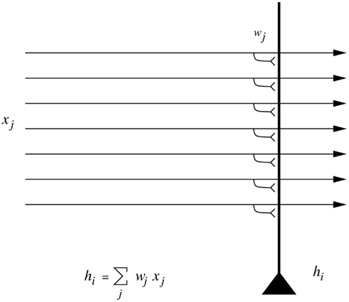
Figure 7. A neuron that computes a dot product of the input pattern with its synaptic weight vector generalizes well to other patterns based on their similarity measured in terms of dot product or correlation, but shows no translation (or size, etc.) invariance.

$h_i=\sum _j{x}_j{w}_{ij}$ (1)

where the sum is over the C input axons, indexed by j.

Now consider translation (or shift) of the input (random binary) pattern vector by one position. The dot product will now drop to a low-level, and the neuron will not respond, even though it is the same pattern, just shifted by one location. This makes the point that special processes are needed to compute invariant representations. Network approaches to such invariant pattern recognition are described in this paper. Once an invariant representation has been computed by a sensory system, it is in a form that is suitable for presentation to a pattern association or autoassociation neural network (Rolls, 2008b).

3.1. Feature Spaces

One very simple possibility for performing object classification is based on feature spaces, which amount to lists of (the extent to which) different features are present in a particular object. The features might consist of textures, colors, areas, ratios of length to width, etc. The spatial arrangement of the features is not taken into account. If n different properties are used to characterize an object, each viewed object is represented by a set of n real numbers. It then becomes possible to represent an object by a point Rⁿ in an n-dimensional space (where R is the resolution of the real numbers used). Such schemes have been investigated (Gibson, 1950, 1979; Selfridge, 1959; Tou and Gonzalez, 1974; Bolles and Cain, 1982; Mundy and Zisserman, 1992; Mel, 1997), but, because the relative positions of the different parts are not implemented in the object recognition scheme, are not sensitive to spatial jumbling of the features. For example, if the features consisted of nose, mouth, and eyes, such a system would respond to faces with jumbled arrangements of the eyes, nose, and mouth, which does not match human vision, nor the responses of macaque inferior temporal cortex neurons, which are sensitive to the spatial arrangement of the features in a face (Rolls et al., 1994). Similarly, such an object recognition system might not distinguish a normal car from a car with the back wheels removed and placed on the roof. Such systems do not therefore perform shape recognition (where shape implies something about the spatial arrangement of features within an object, see further Ullman, 1996), and something more is needed, and is implemented in the primate visual system. However, I note that the features that are present in objects, e.g., a furry texture, are useful to incorporate in object recognition systems, and the brain may well use, and the model VisNet in principle can use, evidence from which features are present in an object as part of the evidence for identification of a particular object. I note that the features might consist also of, for example, the pattern of movement that is characteristic of a particular object (such as a buzzing fly), and might use this as part of the input to final object identification.

The capacity to use shape in invariant object recognition is fundamental to primate vision, but may not be used or fully implemented in the visual systems of some other animals with less developed visual systems. For example, pigeons may correctly identify pictures containing people, a particular person, trees, pigeons, etc. but may fail to distinguish a figure from a scrambled version of a figure (Herrnstein, 1984; Cerella, 1986). Thus their object recognition may be based more on a collection of parts than on a direct comparison of complete figures in which the relative positions of the parts are important. Even if the details of the conclusions reached from this research are revised (Wasserman et al., 1998), it nevertheless does appear that at least some birds may use computationally simpler methods than those needed for invariant shape recognition. For example, it may be that when some birds are trained to discriminate between images in a large set of pictures, they tend to rely on some chance detail of each picture (such as a spot appearing by mistake on the picture), rather than on recognition of the shapes of the object in the picture (Watanabe et al., 1993).

3.2. Structural Descriptions and Syntactic Pattern Recognition

A second approach to object recognition is to decompose the object or image into parts, and to then produce a structural description of the relations between the parts. The underlying assumption is that it is easier to capture object invariances at a level where parts have been identified. This is the type of scheme for which Marr and Nishihara (1978) and Marr (1982) opted (Rolls, 2011a). The particular scheme (Binford, 1981) they adopted consists of generalized cones, series of which can be linked together to form structural descriptions of some, especially animate, stimuli (see Figure 8).

FIGURE 8

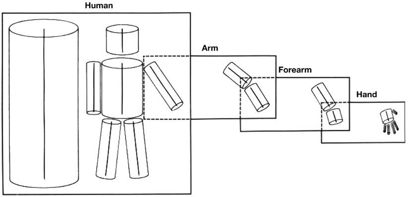
Figure 8. A 3D structural description of an object-based on generalized cone parts. Each box corresponds to a 3D model, with its model axis on the left side of the box and the arrangement of its component axes on the right. In addition, some component axes have 3D models associated with them, as indicated by the way the boxes overlap. (After Marr and Nishihara, 1978.)

Such schemes assume that there is a 3D internal model (structural description) of each object. Perception of the object consists of parsing or segmenting the scene into objects, and then into parts, then producing a structural description of the object, and then testing whether this structural description matches that of any known object stored in the system. Other examples of structural description schemes include those of Sutherland (1968), Winston (1975), and Milner (1974). The relations in the structural description may need to be quite complicated, for example, “connected together,” “inside of,” “larger than,” etc.

Perhaps the most developed model of this type is the recognition by components (RBC) model of Biederman (1987), implemented in a computational model by Hummel and Biederman (1992). His small set (less than 50) of primitive parts named “geons” includes simple 3D shapes such as boxes, cylinders, and wedges. Objects are described by a syntactically linked list of the relations between each of the geons of which they are composed. Describing a table in this way (as a flat top supported by three or four legs) seems quite economical. Other schemes use 2D surface patches as their primitives (Dane and Bajcsy, 1982; Brady et al., 1985; Faugeras and Hebert, 1986; Faugeras, 1993). When 3D objects are being recognized, the implication is that the structural description is a 3D description. This is in contrast to feature hierarchical systems, in which recognition of a 3D object from any view might be accomplished by storing a set of associated 2D views (see below, Section 3.6).

There are a number of difficulties with schemes based on structural descriptions, some general, and some with particular reference to the potential difficulty of their implementation in the brain. First, it is not always easy to decompose the object into its separate parts, which must be performed before the structural description can be produced. For example, it may be difficult to produce a structural description of a cat curled up asleep from separately identifiable parts. Identification of each of the parts is also frequently very difficult when 3D objects are seen from different viewing angles, as key parts may be invisible or highly distorted. This is particularly likely to be difficult in 3D shape perception. It appears that being committed to producing a correct description of the parts before other processes can operate is making too strong a commitment early on in the recognition process.

A second difficulty is that many objects or animals that can be correctly recognized have rather similar structural descriptions. For example, the structural description of many four-legged animals is rather similar. Rather more than a structural description seems necessary to identify many objects and animals.

A third difficulty, which applies especially to biological systems, is the difficulty of implementing the syntax needed to hold the structural description as a 3D model of the object, of producing a syntactic structural description on the fly (in real time, and with potentially great flexibility of the possible arrangement of the parts), and of matching the syntactic description of the object in the image to all the stored representations in order to find a match. An example of a structural description for a limb might be body > thigh > shin > foot > toes. In this description > means “is linked to,” and this link must be between the correct pair of descriptors. If we had just a set of parts, without the syntactic or relational linking, then there would be no way of knowing whether the toes are attached to the foot or to the body. In fact, worse than this, there would be no evidence about what was related to what, just a set of parts. Such syntactical relations are difficult to implement in any biologically plausible neuronal networks used in vision, because if the representations of all the features or parts just mentioned were active simultaneously, how would the spatial relations between the features also be encoded? (How would it be apparent just from the firing of neurons that the toes were linked to the rest of the foot but not to the body?) It would be extremely difficult to implement this “on the fly” syntactic binding in a biologically plausible network (though cf. Hummel and Biederman, 1992), and the only suggested mechanism for flexible syntactic binding, temporal synchronization of the firing of different neurons, is not well supported as a quantitatively important mechanism for information encoding in the ventral visual system, and would have major difficulties in implementing correct, relational, syntactic binding (Section 5.4.1; Rolls, 2008b; Rolls and Treves, 2011).

A fourth difficulty of the structural description approach is that segmentation into objects must occur effectively before object recognition, so that the linked structural description list can be of one object. Given the difficulty of segmenting objects in typical natural cluttered scenes (Ullman, 1996), and the compounding problem of overlap of parts of objects by other objects, segmentation as a first necessary stage of object recognition adds another major difficulty for structural description approaches.

A fifth difficulty is that metric information, such as the relative size of the parts that are linked syntactically, needs to be specified in the structural description (Stan-Kiewicz and Hummel, 1994), which complicates the parts that have to be syntactically linked.

It is because of these difficulties that even in artificial vision systems implemented on computers, where almost unlimited syntactic binding can easily be implemented, the structural description approach to object recognition has not yet succeeded in producing a scheme which actually works in more than an environment in which the types of objects are limited, and the world is far from the natural world, consisting, for example, of 2D scenes (Mundy and Zisserman, 1992).

Although object recognition in the brain is unlikely to be based on the structural description approach, for the reasons given above, and the fact that the evidence described in this paper supports a feature hierarchy rather than the structural description implementation in the brain, it is certainly the case that humans can provide verbal, syntactic, descriptions of objects in terms of the relations of their parts, and that this is often a useful type of description. Humans may therefore, it is suggested, supplement a feature hierarchical object recognition system built into their ventral visual system with the additional ability to use the type of syntax that is necessary for language to provide another level of description of objects. This ability is useful in, for example, engineering applications.

3.3. Template Matching and the Alignment Approach

Another approach is template matching, comparing the image on the retina with a stored image or picture of an object. This is conceptually simple, but there are in practice major problems. One major problem is how to align the image on the retina with the stored images, so that all possible images on the retina can be compared with the stored template or templates of each object.

The basic idea of the alignment approach (Ullman, 1996) is to compensate for the transformations separating the viewed object and the corresponding stored model, and then compare them. For example, the image and the stored model may be similar, except for a difference in size. Scaling one of them will remove this discrepancy and improve the match between them. For a 2D world, the possible transforms are translation (shift), scaling, and rotation. Given, for example, an input letter of the alphabet to recognize, the system might, after segmentation (itself a very difficult process if performed independently of (prior to) object recognition), compensate for translation by computing the center of mass of the object, and shifting the character to a “canonical location.” Scale might be compensated for by calculating the convex hull (the smallest envelope surrounding the object), and then scaling the image. Of course how the shift and scaling would be accomplished is itself a difficult point – easy to perform on a computer using matrix multiplication as in simple computer graphics, but not the sort of computation that could be performed easily or accurately by any biologically plausible network. Compensating for rotation is even more difficult (Ullman, 1996). All this has to happen before the segmented canonical representation of the object is compared to the stored object templates with the same canonical representation. The system of course becomes vastly more complicated when the recognition must be performed of 3D objects seen in a 3D world, for now the particular view of an object after segmentation must be placed into a canonical form, regardless of which view, or how much of any view, may be seen in a natural scene with occluding contours. However, this process is helped, at least in computers that can perform high-precision matrix multiplication, by the fact that (for many continuous transforms such as 3D rotation, translation, and scaling) all the possible views of an object transforming in 3D space can be expressed as the linear combination of other views of the same object (see Chapter 5 of Ullman, 1996; Koenderink and van Doorn, 1991; Koenderink, 1990).

This alignment approach is the main theme of the book by Ullman (1996), and there are a number of computer implementations (Lowe, 1985; Grimson, 1990; Huttenlocher and Ullman, 1990; Shashua, 1995). However, as noted above, it seems unlikely that the brain is able to perform the high-precision calculations needed to perform the transforms required to align any view of a 3D object with some canonical template representation. For this reason, and because the approach also relies on segmentation of the object in the scene before the template alignment algorithms can start, and because key features may need to be correctly identified to be used in the alignment (Edelman, 1999), this approach is not considered further here.

We may note here in passing that some animals with a less computationally developed visual system appear to attempt to solve the alignment problem by actively moving their heads or eyes to see what template fits, rather than starting with an image on the eye and attempting to transform it into canonical coordinates. This “active vision” approach used, for example, by some invertebrates has been described by Land (1999) and Land and Collett (1997).

3.4. Some Further Machine Learning Approaches

Learning the transformations and invariances of the signal is another approach to invariant object recognition at the interface of machine learning and theoretical neuroscience. For example, rather than focusing on the templates, “map-seeking circuit theory” focuses on the transforms (Arathorn, 2002, 2005). The theory provides a general computational mechanism for discovery of correspondences in massive transformation spaces by exploiting an ordering property of superpositions. The latter allows a set of transformations of an input image to be formed into a sequence of superpositions which are then “culled” to a composition of single mappings by a competitive process which matches each superposition against a superposition of inverse transformations of memory patterns. Earlier work considered how to minimize the variance in the output when the image transformed (Leen, 1995). Another approach is to add transformation invariance to mixture models, by approximating the non-linear transformation manifold by a discrete set of points (Frey and Jojic, 2003). They showed how the expectation maximization algorithm can be used to jointly learn clusters, while at the same time inferring the transformation associated with each input. In another approach, an unsupervised algorithm for learning Lie group operators for in-plane transforms from input data was described (Rao and Ruderman, 1999).

3.5. Networks that Can Reconstruct Their Inputs

Hinton et al. (1995) and Hinton and Ghahramani (1997) have argued that cortical computation is invertible, so that, for example, the forward transform of visual information from V1 to higher areas loses no information, and there can be a backward transform from the higher areas to V1. A comparison of the reconstructed representation in V1 with the actual image from the world might in principle be used to correct all the synaptic weights between the two (in both the forward and the reverse directions), in such a way that there are no errors in the transform (Hinton, 2010). This suggested reconstruction scheme would seem to involve non-local synaptic weight correction (though see Hinton and Sejnowski, 1986; O’Reilly and Munakata, 2000) for a suggested, although still biologically implausible, neural implementation, contrastive Hebbian learning), or other biologically implausible operations. The scheme also does not seem to provide an account for why or how the responses of inferior temporal cortex neurons become the way they are (providing information about which object is seen relatively independently of position on the retina, size, or view). The whole forward transform performed in the brain seems to lose much of the information about the size, position, and view of the object, as it is evidence about which object is present invariant of its size, view, etc. that is useful to the stages of processing about objects that follow (Rolls, 2008b). Because of these difficulties, and because the backprojections are needed for processes such as recall (Rolls, 2008b), this approach is not considered further here.

In the context of recall, if the visual system were to perform a reconstruction in V1 of a visual scene from what is represented in the inferior temporal visual cortex, then it might be supposed that remembered visual scenes might be as information-rich (and subjectively as full of rich detail) as seeing the real thing. This is not the case for most humans, and indeed this point suggests that at least what reaches consciousness from the inferior temporal visual cortex (which is activated during the recall of visual memories) is the identity of the object (as made explicit in the firing rate of the neurons), and not the low-level details of the exact place, size, and view of the object in the recalled scene, even though, according to the reconstruction argument, that information should be present in the inferior temporal visual cortex.

3.6. Feature Hierarchies and 2D View-Based Object Recognition

Another approach, and one that is much closer to what appears to be present in the primate ventral visual system (Wurtz and Kandel, 2000a; Rolls and Deco, 2002; Rolls, 2008b), is a feature hierarchy system (see Figure 9).

FIGURE 9

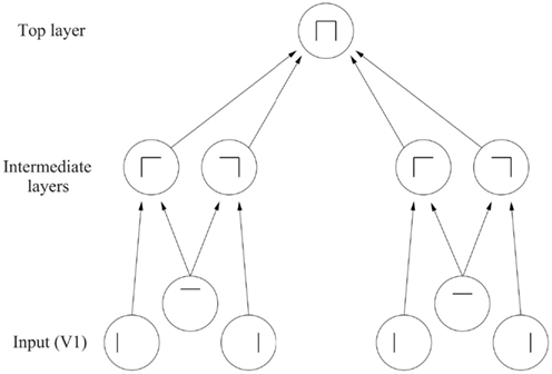
Figure 9. The feature hierarchy approach to object recognition. The inputs may be neurons tuned to oriented straight line segments. In early intermediate-layers neurons respond to a combination of these inputs in the correct spatial position with respect to each other. In further intermediate layers, of which there may be several, neurons respond with some invariance to the feature combinations represented early, and form higher order feature combinations. Finally, in the top layer, neurons respond to combinations of what is represented in the preceding intermediate layer, and thus provide evidence about objects in a position (and scale and even view) invariant way. Convergence through the network is designed to provide top layer neurons with information from across the entire input retina, as part of the solution to translation invariance, and other types of invariance are treated similarly.

In this approach, the system starts with some low-level description of the visual scene, in terms, for example, of oriented straight line segments of the type that are represented in the responses of primary visual cortex (V1) neurons, and then builds in repeated hierarchical layers features based on what is represented in previous layers. A feature may thus be defined as a combination of what is represented in the previous layer. For example, after V1, features might consist of combinations of straight lines, which might represent longer curved lines (Zucker et al., 1989), or terminated lines (in fact represented in V1 as end-stopped cells), corners, “T” junctions which are characteristic of obscuring edges, and (at least in humans) the arrow and “Y” vertices which are characteristic properties of man-made environments. Evidence that such feature combination neurons are present in V2 is that some neurons respond to combinations of line elements that join at different angles (Hegde and Van Essen, 2000, 2003, 2007; Ito and Komatsu, 2004; Anzai et al., 2007). (An example of this might be a neuron responding to a “V” shape at a particular orientation.) As one ascends the hierarchy, neurons might respond to more complex trigger features. For example, two parts of a complex figure may need to be in the correct spatial arrangement with respect to each other, as shown by Tanaka (1996) for V4 and posterior inferior temporal cortex neurons. In another example, V4 neurons may respond to the curvature of the elements of a stimulus (Carlson et al., 2011). Further on, neurons might respond to combinations of several such intermediate-level feature combination neurons, and thus come to respond systematically differently to different objects, and thus to convey information about which object is present. This approach received neurophysiological support early on from the results of Hubel and Wiesel (1962) and Hubel and Wiesel (1968) in the cat and monkey, and many of the data described in Chapter 5 of Rolls and Deco (2002) are consistent with this scheme.

A number of problems need to be solved for such feature hierarchy visual systems to provide a useful model of object recognition in the primate visual system.

First, some way needs to be found to keep the number of feature combination neurons realistic at each stage, without undergoing a combinatorial explosion. If a separate feature combination neuron was needed to code for every possible combination of n types of feature each with a resolution of 2 levels (binary encoding) in the preceding stage, then 2ⁿ neurons would be needed. The suggestion that is made in Section 4 is that by forming neurons that respond to low-order combinations of features (neurons that respond to just say 2–4 features from the preceding stage), the number of actual feature analyzing neurons can be kept within reasonable numbers. By reasonable we mean the number of neurons actually found at any one stage of the visual system, which, for V4 might be in the order of 60 × 10⁶ neurons (assuming a volume for macaque V4 of approximately 2,000 mm³, and a cell density of 20,000–40,000 neurons per mm³, Rolls, 2008b). This is certainly a large number; but the fact that a large number of neurons is present at each stage of the primate visual system is in fact consistent with the hypothesis that feature combination neurons are part of the way in which the brain solves object recognition. A factor which also helps to keep the number of neurons under control is the statistics of the visual world, which contain great redundancies. The world is not random, and indeed the statistics of natural images are such that many regularities are present (Field, 1994), and not every possible combination of pixels on the retina needs to be separately encoded. A third factor which helps to keep the number of connections required onto each neuron under control is that in a multilayer hierarchy each neuron can be set up to receive connections from only a small region of the preceding layer. Thus an individual neuron does not need to have connections from all the neurons in the preceding layer. Over multiple-layers, the required convergence can be produced so that the same neurons in the top layer can be activated by an image of an effective object anywhere on the retina (see Figure 1).

A second problem of feature hierarchy approaches is how to map all the different possible images of an individual object through to the same set of neurons in the top layer by modifying the synaptic connections (see Figure 1). The solution discussed in Sections 4, 5.1.1, and 5.3 is the use of a synaptic modification rule with a short-term memory trace of the previous activity of the neuron, to enable it to learn to respond to the now transformed version of what was seen very recently, which, given the statistics of looking at the visual world, will probably be an input from the same object.

A third problem of feature hierarchy approaches is how they can learn in just a few seconds of inspection of an object to recognize it in different transforms, for example, in different positions on the retina in which it may never have been presented during training. A solution to this problem is provided in Section 5.4, in which it is shown that this can be a natural property of feature hierarchy object recognition systems, if they are trained first for all locations on the intermediate-level feature combinations of which new objects will simply be a new combination, and therefore requiring learning only in the upper layers of the hierarchy.

A fourth potential problem of feature hierarchy systems is that when solving translation invariance they need to respond to the same local spatial arrangement of features (which are needed to specify the object), but to ignore the global position of the whole object. It is shown in Section 5.4 that feature hierarchy systems can solve this problem by forming feature combination neurons at an early stage of processing (e.g., V1 or V2 in the brain) that respond with high-spatial precision to the local arrangement of features. Such neurons would respond differently, for example, to L, +, and T if they receive inputs from two line-responding neurons. It is shown in Section 5.4 that at later layers of the hierarchy, where some of the intermediate-level feature combination neurons are starting to show translation invariance, then correct object recognition may still occur because only one object contains just those sets of intermediate-level neurons in which the spatial representation of the features is inherent in the encoding.

The type of representation developed in a hierarchical object recognition system, in the brain, and by VisNet as described in the rest of this paper would be suitable for recognition of an object, and for linking associative memories to objects, but would be less good for making actions in 3D space to particular parts of, or inside, objects, as the 3D coordinates of each part of the object would not be explicitly available. It is therefore proposed that visual fixation is used to locate in foveal vision part of an object to which movements must be made, and that local disparity and other measurements of depth (made explicit in the dorsal visual system) then provide sufficient information for the motor system to make actions relative to the small part of space in which a local, view-dependent, representation of depth would be provided (cf. Ballard, 1990).

One advantage of feature hierarchy systems is that they can operate fast (Rolls, 2008b).

A second advantage is that the feature analyzers can be built out of the rather simple competitive networks (Rolls, 2008b) which use a local learning rule, and have no external teacher, so that they are rather biologically plausible. Another advantage is that, once trained on subset features common to most objects, the system can then learn new objects quickly.

A related third advantage is that, if implemented with competitive nets as in the case of VisNet (see Section 5), then neurons are allocated by self-organization to represent just the features present in the natural statistics of real images (cf. Field, 1994), and not every possible feature that could be constructed by random combinations of pixels on the retina.

A related fourth advantage of feature hierarchy networks is that because they can utilize competitive networks, they can still produce the best guess at what is in the image under non-ideal conditions, when only parts of objects are visible because, for example, of occlusion by other objects, etc. The reasons for this are that competitive networks assess the evidence for the presence of certain “features” to which they are tuned using a dot product operation on their inputs, so that they are inherently tolerant of missing input evidence; and reach a state that reflects the best hypothesis or hypotheses (with soft competition) given the whole set of inputs, because there are competitive interactions between the different neurons (Rolls, 2008b).

A fifth advantage of a feature hierarchy system is that, as shown in Section 5.5, the system does not need to perform segmentation into objects as part of pre-processing, nor does it need to be able to identify parts of an object, and can also operate in cluttered scenes in which the object may be partially obscured. The reason for this is that once trained on objects, the system then operates somewhat like an associative memory, mapping the image properties forward onto whatever it has learned about before, and then by competition selecting just the most likely output to be activated. Indeed, the feature hierarchy approach provides a mechanism by which processing at the object recognition level could feed back using backprojections to early cortical areas to provide top-down guidance to assist segmentation. Although backprojections are not built into VisNet2 (Rolls and Milward, 2000), they have been added when attentional top-down processing must be incorporated (Deco and Rolls, 2004), are present in the brain, and are incorporated into the models described elsewhere (Rolls, 2008b). Although the operation of the ventral visual system can proceed as a feed-forward hierarchy, as shown by backward masking experiments (Rolls and Tovee, 1994; Rolls et al., 1999; Rolls, 2003, 2006), top-down influences can of course be implemented by the backprojections, and may be useful in further shaping the activity of neurons at lower levels in the hierarchy based on the neurons firing at a higher level as a result of dynamical interactions of neurons at different layers of the hierarchy (Rolls, 2008b; Jiang et al., 2011).

A sixth advantage of feature hierarchy systems is that they can naturally utilize features in the images of objects which are not strictly part of a shape description scheme, such as the fact that different objects have different textures, colors, etc. Feature hierarchy systems, because they utilize whatever is represented at earlier stages in forming feature combination neurons at the next stage, naturally incorporate such “feature list” evidence into their analysis, and have the advantages of that approach (see Section 3.1 and also Mel, 1997). Indeed, the feature space approach can utilize a hybrid representation, some of whose dimensions may be discrete and defined in structural terms, while other dimensions may be continuous and defined in terms of metric details, and others may be concerned with non-shape properties such as texture and color (cf. Edelman, 1999).

A seventh advantage of feature hierarchy systems is that they do not need to utilize “on the fly” or run-time arbitrary binding of features. Instead, the spatial syntax is effectively hard-wired into the system when it is trained, in that the feature combination neurons have learned to respond to their set of features when they are in a given spatial arrangement on the retina.

An eighth advantage of feature hierarchy systems is that they can self-organize (given the right functional architecture, trace synaptic learning rule, and the temporal statistics of the normal visual input from the world), with no need for an external teacher to specify that the neurons must learn to respond to objects. The correct, object, representation self-organizes itself given rather economically specified genetic rules for building the network (cf. Rolls and Stringer, 2000).

Ninth, it is also noted that hierarchical visual systems may recognize 3D objects based on a limited set of 2D views of objects, and that the same architectural rules just stated and implemented in VisNet will correctly associate together the different views of an object. It is part of the concept (see below), and consistent with neurophysiological data (Tanaka, 1996), that the neurons in the upper layers will generalize correctly within a view (see Section 5.6).

After the immediately following description of early models of a feature hierarchy approach implemented in the Cognitron and Neocognitron, we turn for the remainder of this paper to analyses of how a feature hierarchy approach to invariant visual object recognition might be implemented in the brain, and how key computational issues could be solved by such a system. The analyses are developed and tested with a model, VisNet, which will shortly be described. Much of the data we have on the operation of the high-order visual cortical areas (Section 2; Rolls and Deco, 2002; Anzai et al., 2007; Rolls, 2008b) suggest that they implement a feature hierarchy approach to visual object recognition, as is made evident in the remainder of this paper.

3.6.1. The cognitron and neocognitron

An early computational model of a hierarchical feature-based approach to object recognition, joining other early discussions of this approach (Selfridge, 1959; Sutherland, 1968; Barlow, 1972; Milner, 1974), was proposed by Fukushima (1975, 1980, 1989, 1991). His model used two types of cell within each layer to approach the problem of invariant representations. In each layer, a set of “simple cells,” with defined position, orientation, etc. sensitivity for the stimuli to which they responded, was followed by a set of “complex cells,” which generalized a little over position, orientation, etc. This simple cell – complex cell pairing within each layer provided some invariance. When a neuron in the network using competitive learning with its stimulus set, which was typically letters on a 16 × 16 pixel array, learned that a particular feature combination had occurred, that type of feature analyzer was replicated in a non-local manner throughout the layer, to provide further translation invariance. Invariant representations were thus learned in a different way from VisNet. Up to eight layers were used. The network could learn to differentiate letters, even with some translation, scaling, or distortion. Although internally it is organized and learns very differently to VisNet, it is an independent example of the fact that useful invariant pattern recognition can be performed by multilayer hierarchical networks. A major biological implausibility of the system is that once one neuron within a layer learned, other similar neurons were set up throughout the layer by a non-local process. A second biological limitation was that no learning rule or self-organizing process was specified as to how the complex cells can provide translation-invariant representations of simple cell responses – this was simply handwired. Solutions to both these issues are provided by VisNet.

4. Hypotheses about the Computational Mechanisms in the Visual Cortex for Object Recognition

The neurophysiological findings described in Section 2, and wider considerations on the possible computational properties of the cerebral cortex (Rolls, 1992, 2000, 2008b; Rolls and Treves, 1998; Rolls and Deco, 2002), lead to the following outline working hypotheses on object recognition by visual cortical mechanisms (see Rolls, 1992). The principles underlying the processing of faces and other objects may be similar, but more neurons may become allocated to represent different aspects of faces because of the need to recognize the faces of many different individuals, that is to identify many individuals within the category faces.

Cortical visual processing for object recognition is considered to be organized as a set of hierarchically connected cortical regions consisting at least of V1, V2, V4, posterior inferior temporal cortex (TEO), inferior temporal cortex (e.g., TE3, TEa, and TEm), and anterior temporal cortical areas (e.g., TE2 and TE1). (This stream of processing has many connections with a set of cortical areas in the anterior part of the superior temporal sulcus, including area TPO.) There is convergence from each small part of a region to the succeeding region (or layer in the hierarchy) in such a way that the receptive field sizes of neurons (e.g., 1° near the fovea in V1) become larger by a factor of approximately 2.5 with each succeeding stage (and the typical parafoveal receptive field sizes found would not be inconsistent with the calculated approximations of, e.g., 8° in V4, 20° in TEO, and 50° in the inferior temporal cortex Boussaoud et al., 1991; see Figure 1). Such zones of convergence would overlap continuously with each other (see Figure 1). This connectivity would be part of the architecture by which translation-invariant representations are computed.

Each layer is considered to act partly as a set of local self-organizing competitive neuronal networks with overlapping inputs. (The region within which competition would be implemented would depend on the spatial properties of inhibitory interneurons, and might operate over distances of 1–2 mm in the cortex.) These competitive nets operate by a single set of forward inputs leading to (typically non-linear, e.g., sigmoid) activation of output neurons; of competition between the output neurons mediated by a set of feedback inhibitory interneurons which receive from many of the principal (in the cortex, pyramidal) cells in the net and project back (via inhibitory interneurons) to many of the principal cells and serve to decrease the firing rates of the less active neurons relative to the rates of the more active neurons; and then of synaptic modification by a modified Hebb rule, such that synapses to strongly activated output neurons from active input axons strengthen, and from inactive input axons weaken (Rolls, 2008b). A biologically plausible form of this learning rule that operates well in such networks is

$\delta w_{ij}=\alpha y_i\left(x_j-w_{ij}\right)$ (2)

where $\delta w_{ij}$ is the change of the synaptic weight, α is a learning rate constant, $y_i$ is the firing rate of the ith postsynaptic neuron, and $x_j$ and $w_{ij}$ are in appropriate units (Rolls, 2008b). Such competitive networks operate to detect correlations between the activity of the input neurons, and to allocate output neurons to respond to each cluster of such correlated inputs. These networks thus act as categorizers. In relation to visual information processing, they would remove redundancy from the input representation, and would develop low-entropy representations of the information (cf. Barlow, 1985; Barlow et al., 1989). Such competitive nets are biologically plausible, in that they utilize Hebb-modifiable forward excitatory connections, with competitive inhibition mediated by cortical inhibitory neurons. The competitive scheme I suggest would not result in the formation of “winner-take-all” or “grandmother” cells, but would instead result in a small ensemble of active neurons representing each input (Rolls and Treves, 1998; Rolls, 2008b). The scheme has the advantages that the output neurons learn better to distribute themselves between the input patterns (cf. Bennett, 1990), and that the sparse representations formed have utility in maximizing the number of memories that can be stored when, toward the end of the visual system, the visual representation of objects is interfaced to associative memory (Rolls and Treves, 1998; Rolls, 2008b).

Translation invariance would be computed in such a system by utilizing competitive learning to detect regularities in inputs when real objects are translated in the physical world. The hypothesis is that because objects have continuous properties in space and time in the world, an object at one place on the retina might activate feature analyzers at the next stage of cortical processing, and when the object was translated to a nearby position, because this would occur in a short period (e.g., 0.5 s), the membrane of the post-synaptic neuron would still be in its “Hebb-modifiable” state (caused, for example, by calcium entry as a result of the voltage-dependent activation of NMDA receptors), and the presynaptic afferents activated with the object in its new position would thus become strengthened on the still-activated post-synaptic neuron. It is suggested that the short temporal window (e.g., 0.5 s) of Hebb-modifiability helps neurons to learn the statistics of objects moving in the physical world, and at the same time to form different representations of different feature combinations or objects, as these are physically discontinuous and present less regular correlations to the visual system. Földiák (1991) has proposed computing an average activation of the post-synaptic neuron to assist with the same problem. One idea here is that the temporal properties of the biologically implemented learning mechanism are such that it is well suited to detecting the relevant continuities in the world of real objects. Another suggestion is that a memory trace for what has been seen in the last 300 ms appears to be implemented by a mechanism as simple as continued firing of inferior temporal neurons after the stimulus has disappeared, as has been found in masking experiments (Rolls and Tovee, 1994; Rolls et al., 1994, 1999; Rolls, 2003).

I also suggested (Rolls, 1992) that other invariances, for example, size, spatial-frequency, and rotation invariance, could be learned by a comparable process. (Early processing in V1 which enables different neurons to represent inputs at different spatial scales would allow combinations of the outputs of such neurons to be formed at later stages. Scale invariance would then result from detecting at a later stage which neurons are almost conjunctively active as the size of an object alters.) It is suggested that this process takes place at each stage of the multiple-layer cortical processing hierarchy, so that invariances are learned first over small regions of space, and then over successively larger regions. This limits the size of the connection space within which correlations must be sought.

Increasing complexity of representations could also be built in such a multiple-layer hierarchy by similar mechanisms. At each stage or layer the self-organizing competitive nets would result in combinations of inputs becoming the effective stimuli for neurons. In order to avoid the combinatorial explosion, it is proposed, following Feldman (1985), that low-order combinations of inputs would be what is learned by each neuron. (Each input would not be represented by activity in a single input axon, but instead by activity in a set of active input axons.) Evidence consistent with this suggestion that neurons are responding to combinations of a few variables represented at the preceding stage of cortical processing is that some neurons in V1 respond to combinations of bars or edges (Shevelev et al., 1995; Sillito et al., 1995); V2 and V4 respond to end-stopped lines, to angles formed by a combination of lines, to tongues flanked by inhibitory subregions, or to combinations of colors (Hegde and Van Essen, 2000, 2003, 2007; Ito and Komatsu, 2004; Anzai et al., 2007; Orban, 2011); in posterior inferior temporal cortex to stimuli which may require two or more simple features to be present (Tanaka et al., 1990); and in the temporal cortical face processing areas to images that require the presence of several features in a face (such as eyes, hair, and mouth) in order to respond (Perrett et al., 1982; Yamane et al., 1988; Rolls, 2011b; see Figure 6). (Precursor cells to face-responsive neurons might, it is suggested, respond to combinations of the outputs of the neurons in V1 that are activated by faces, and might be found in areas such as V4.) It is an important part of this suggestion that some local spatial information would be inherent in the features which were being combined. For example, cells might not respond to the combination of an edge and a small circle unless they were in the correct spatial relation to each other. (This is in fact consistent with the data of Tanaka et al. (1990), and with our data on face neurons, in that some face neurons require the face features to be in the correct spatial configuration, and not jumbled, Rolls et al. (1994).) The local spatial information in the features being combined would ensure that the representation at the next level would contain some information about the (local) arrangement of features. Further low-order combinations of such neurons at the next stage would include sufficient local spatial information so that an arbitrary spatial arrangement of the same features would not activate the same neuron, and this is the proposed, and limited, solution which this mechanism would provide for the feature binding problem (Elliffe et al., 2002; cf. von der Malsburg, 1990). By this stage of processing a view-dependent representation of objects suitable for view-dependent processes such as behavioral responses to face expression and gesture would be available.

It is suggested that view-independent representations could be formed by the same type of computation, operating to combine a limited set of views of objects. The plausibility of providing view-independent recognition of objects by combining a set of different views of objects has been proposed by a number of investigators (Koenderink and Van Doorn, 1979; Poggio and Edelman, 1990; Logothetis et al., 1994; Ullman, 1996). Consistent with the suggestion that the view-independent representations are formed by combining view-dependent representations in the primate visual system, is the fact that in the temporal cortical areas, neurons with view-independent representations of faces are present in the same cortical areas as neurons with view-dependent representations (from which the view-independent neurons could receive inputs; Perrett et al., 1985; Hasselmo et al., 1989b; Booth and Rolls, 1998). This solution to “object-based” representations is very different from that traditionally proposed for artificial vision systems, in which the coordinates in 3D space of objects are stored in a database, and general-purpose algorithms operate on these to perform transforms such as translation, rotation, and scale change in 3D space (e.g., Marr, 1982). In the present, much more limited but more biologically plausible scheme, the representation would be suitable for recognition of an object, and for linking associative memories to objects, but would be less good for making actions in 3D space to particular parts of, or inside, objects, as the 3D coordinates of each part of the object would not be explicitly available. It is therefore proposed that visual fixation is used to locate in foveal vision part of an object to which movements must be made, and that local disparity and other measurements of depth then provide sufficient information for the motor system to make actions relative to the small part of space in which a local, view-dependent, representation of depth would be provided (cf. Ballard, 1990).

The computational processes proposed above operate by an unsupervised learning mechanism, which utilizes statistical regularities in the physical environment to enable representations to be built. In some cases it may be advantageous to utilize some form of mild teaching input to the visual system, to enable it to learn, for example, that rather similar visual inputs have very different consequences in the world, so that different representations of them should be built. In other cases, it might be helpful to bring representations together, if they have identical consequences, in order to use storage capacity efficiently. It is proposed elsewhere (Rolls, 1989a,b, 2008b; Rolls and Treves, 1998) that the backprojections from each adjacent cortical region in the hierarchy (and from the amygdala and hippocampus to higher regions of the visual system) play such a role by providing guidance to the competitive networks suggested above to be important in each cortical area. This guidance, and also the capability for recall, are it is suggested implemented by Hebb-modifiable connections from the backprojecting neurons to the principal (pyramidal) neurons of the competitive networks in the preceding stages (Rolls, 1989a,b, 2008b; Rolls and Treves, 1998).

The computational processes outlined above use sparse distributed coding with relatively finely tuned neurons with a graded response region centered about an optimal response achieved when the input stimulus matches the synaptic weight vector on a neuron. The distributed nature of the coding but with fine tuning would help to limit the combinatorial explosion, to keep the number of neurons within the biological range. The graded response region would be crucial in enabling the system to generalize correctly to solve, for example, the invariances. However, such a system would need many neurons, each with considerable learning capacity, to solve visual perception in this way. This is fully consistent with the large number of neurons in the visual system, and with the large number of, probably modifiable, synapses on each neuron (e.g., 10,000). Further, the fact that many neurons are tuned in different ways to faces is consistent with the fact that in such a computational system, many neurons would need to be sensitive (in different ways) to faces, in order to allow recognition of many individual faces when all share a number of common properties.

5. The Feature Hierarchy Approach to Invariant Object Recognition: Computational Issues

The feature hierarchy approach to invariant object recognition was introduced in Section 3.6, and advantages and disadvantages of it were discussed. Hypotheses about how object recognition could be implemented in the brain which are consistent with much of the neurophysiology discussed in Section 2 and by Rolls and Deco (2002) and Rolls (2008b) were set out in Section 4. These hypotheses effectively incorporate a feature hierarchy system while encompassing much of the neurophysiological evidence. In this Section (5), we consider the computational issues that arise in such feature hierarchy systems, and in the brain systems that implement visual object recognition. The issues are considered with the help of a particular model, VisNet, which requires precise specification of the hypotheses, and at the same time enables them to be explored and tested numerically and quantitatively. However, I emphasize that the issues to be covered in Section 5 are key and major computational issues for architectures of this feature hierarchical type (Rolls, 2008b), and are very relevant to understanding how invariant object recognition is implemented in the brain.

VisNet is a model of invariant object recognition based on Rolls’ (Rolls, 1992) hypotheses. It is a computer simulation that allows hypotheses to be tested and developed about how multilayer hierarchical networks of the type believed to be implemented in the visual cortical pathways operate. The architecture captures a number of aspects of the architecture of the visual cortical pathways, and is described next. The model of course, as with all models, requires precise specification of what is to be implemented, and at the same time involves specified simplifications of the real architecture, as investigations of the fundamental aspects of the information processing being performed are more tractable in a simplified and at the same time quantitatively specified model. First the architecture of the model is described, and this is followed by descriptions of key issues in such multilayer feature hierarchical models, such as the issue of feature binding, the optimal form of training rule for the whole system to self-organize, the operation of the network in natural environments and when objects are partly occluded, how outputs about individual objects can be read out from the network, and the capacity of the system.

5.1. The Architecture of VisNet

Fundamental elements of Rolls’ (1992) theory for how cortical networks might implement invariant object recognition are described in Section 4. They provide the basis for the design of VisNet, and can be summarized as:

• A series of competitive networks, organized in hierarchical layers, exhibiting mutual inhibition over a short range within each layer. These networks allow combinations of features or inputs occurring in a given spatial arrangement to be learned by neurons, ensuring that higher order spatial properties of the input stimuli are represented in the network.

• A convergent series of connections from a localized population of cells in preceding layers to each cell of the following layer, thus allowing the receptive field size of cells to increase through the visual processing areas or layers.

• A modified Hebb-like learning rule incorporating a temporal trace of each cell’s previous activity, which, it is suggested, will enable the neurons to learn transform invariances.

The first two elements of Rolls’ theory are used to constrain the general architecture of a network model, VisNet, of the processes just described that is intended to learn invariant representations of objects. The simulation results described in this paper using VisNet show that invariant representations can be learned by the architecture. It is moreover shown that successful learning depends crucially on the use of the modified Hebb rule. The general architecture simulated in VisNet, and the way in which it allows natural images to be used as stimuli, has been chosen to enable some comparisons of neuronal responses in the network and in the brain to similar stimuli to be made.

5.1.1. The trace rule

The learning rule implemented in the VisNet simulations utilizes the spatio-temporal constraints placed upon the behavior of “real-world” objects to learn about natural object transformations. By presenting consistent sequences of transforming objects the cells in the network can learn to respond to the same object through all of its naturally transformed states, as described by Földiák (1991), Rolls (1992), Wallis et al. (1993), and Wallis and Rolls (1997). The learning rule incorporates a decaying trace of previous cell activity and is henceforth referred to simply as the “trace” learning rule. The learning paradigm we describe here is intended in principle to enable learning of any of the transforms tolerated by inferior temporal cortex neurons, including position, size, view, lighting, and spatial-frequency (Rolls, 1992, 2000, 2008b; Rolls and Deco, 2002).

To clarify the reasoning behind this point, consider the situation in which a single neuron is strongly activated by a stimulus forming part of a real-world object. The trace of this neuron’s activation will then gradually decay over a time period in the order of 0.5 s. If, during this limited time window, the net is presented with a transformed version of the original stimulus then not only will the initially active afferent synapses modify onto the neuron, but so also will the synapses activated by the transformed version of this stimulus. In this way the cell will learn to respond to either appearance of the original stimulus. Making such associations works in practice because it is very likely that within short-time periods different aspects of the same object will be being inspected. The cell will not, however, tend to make spurious links across stimuli that are part of different objects because of the unlikelihood in the real-world of one object consistently following another.

Various biological bases for this temporal trace have been advanced as follows: [The precise mechanisms involved may alter the precise form of the trace rule which should be used. Földiák (1992) describes an alternative trace rule which models individual NMDA channels. Equally, a trace implemented by extended cell firing should be reflected in representing the trace as an external firing rate, rather than an internal signal.]

• The persistent firing of neurons for as long as 100–400 ms observed after presentations of stimuli for 16 ms (Rolls and Tovee, 1994) could provide a time window within which to associate subsequent images. Maintained activity may potentially be implemented by recurrent connections between as well as within cortical areas (Rolls and Treves, 1998; Rolls and Deco, 2002; Rolls, 2008b). [The prolonged firing of inferior temporal cortex neurons during memory delay periods of several seconds, and associative links reported to develop between stimuli presented several seconds apart (Miyashita, 1988) are on too long a time scale to be immediately relevant to the present theory. In fact, associations between visual events occurring several seconds apart would, under normal environmental conditions, be detrimental to the operation of a network of the type described here, because they would probably arise from different objects. In contrast, the system described benefits from associations between visual events which occur close in time (typically within 1 s), as they are likely to be from the same object.]

• The binding period of glutamate in the NMDA channels, which may last for 100 ms or more, may implement a trace rule by producing a narrow time window over which the average activity at each presynaptic site affects learning (Hestrin et al., 1990; Földiák, 1992; Rhodes, 1992; Rolls, 1992; Spruston et al., 1995).

• Chemicals such as nitric oxide may be released during high neural activity and gradually decay in concentration over a short-time window during which learning could be enhanced (Montague et al., 1991; Földiák, 1992; Garthwaite, 2008).

The trace update rule used in the baseline simulations of VisNet (Wallis and Rolls, 1997) is equivalent to both Földiák’s used in the context of translation invariance (Wallis et al., 1993) and to the earlier rule of Sutton and Barto (1981) explored in the context of modeling the temporal properties of classical conditioning, and can be summarized as follows:

$\delta w_j=\alpha {\overline{y}}^{\tau }{x}_j$ (3)

where

${\overline{y}}^{\tau }=\left(1-\eta \right)y^{\tau }+\eta {\overline{y}}^{\tau -1}$ (4)

and

To bound the growth of each neuron’s synaptic weight vector, w _i for the ith neuron, its length is explicitly normalized (a method similarly employed by von der Malsburg (1973) which is commonly used in competitive networks (Rolls, 2008b). An alternative, more biologically relevant implementation, using a local weight bounding operation which utilizes a form of heterosynaptic long-term depression (Rolls, 2008b), has in part been explored using a version of the Oja (1982) rule (see Wallis and Rolls, 1997).

5.1.2. The network implemented in VisNet

The network itself is designed as a series of hierarchical, convergent, competitive networks, in accordance with the hypotheses advanced above. The actual network consists of a series of four layers, constructed such that the convergence of information from the most disparate parts of the network’s input layer can potentially influence firing in a single neuron in the final layer – see Figure 1. This corresponds to the scheme described by many researchers (Rolls, 1992, 2008b; Van Essen et al., 1992) as present in the primate visual system – see Figure 1. The forward connections to a cell in one-layer are derived from a topologically related and confined region of the preceding layer. The choice of whether a connection between neurons in adjacent layers exists or not is based upon a Gaussian distribution of connection probabilities which roll off radially from the focal point of connections for each neuron. (A minor extra constraint precludes the repeated connection of any pair of cells.) In particular, the forward connections to a cell in one layer come from a small region of the preceding layer defined by the radius in Table 1 which will contain approximately 67% of the connections from the preceding layer. Table 1 shows the dimensions for VisNetL, the system we are currently using (Perry et al., 2010), which is a (16×) larger version of the version of VisNet than used in most of our previous investigations, which utilized 32 × 32 neurons per layer. Figure 1 shows the general convergent network architecture used. Localization and limitation of connectivity in the network is intended to mimic cortical connectivity, partially because of the clear retention of retinal topology through regions of visual cortex. This architecture also encourages the gradual combination of features from layer to layer which has relevance to the binding problem, as described in Section 5.4.

TABLE 1

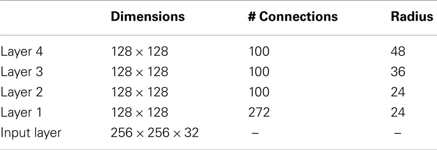
Table 1. VisNet dimensions.

Modeling topological constraints in connectivity leads to an issue concerning neurons at the edges of the network layers. In principle these neurons may either receive no input from beyond the edge of the preceding layer, or have heir connections repeatedly sample neurons at the edge of the previous layer. In practice either solution is liable to introduce artificial weighting on the few active inputs at the edge and hence cause the edge to have unwanted influence over the development of the network as a whole. In the real brain such edge-effects would be naturally smoothed by the transition of the locus of cellular input from the fovea to the lower acuity periphery of the visual field. However, it poses a problem here because we are in effect only simulating the small high-acuity foveal portion of the visual field in our simulations. As an alternative to the former solutions Wallis and Rolls (1997) elected to form the connections into a toroid, such that connections wrap back onto the network from opposite sides. This wrapping happens at all four layers of the network, and in the way an image on the “retina” is mapped to the input filters. This solution has the advantage of making all of the boundaries effectively invisible to the network. Further, this procedure does not itself introduce problems into evaluation of the network for the problems set, as many of the critical comparisons in VisNet involve comparisons between a network with the same architecture trained with the trace rule, or with the Hebb rule, or not trained at all. In practice, it is shown below that only the network trained with the trace rule solves the problem of forming invariant representations.

5.1.3. Competition and lateral inhibition

In order to act as a competitive network some form of mutual inhibition is required within each layer, which should help to ensure that all stimuli presented are evenly represented by the neurons in each layer. This is implemented in VisNet by a form of lateral inhibition. The idea behind the lateral inhibition, apart from this being a property of cortical architecture in the brain, was to prevent too many neurons that received inputs from a similar part of the preceding layer responding to the same activity patterns. The purpose of the lateral inhibition was to ensure that different receiving neurons coded for different inputs. This is important in reducing redundancy (Rolls, 2008b). The lateral inhibition is conceived as operating within a radius that was similar to that of the region within which a neuron received converging inputs from the preceding layer (because activity in one zone of topologically organized processing within a layer should not inhibit processing in another zone in the same layer, concerned perhaps with another part of the image). [Although the extent of the lateral inhibition actually investigated by Wallis and Rolls (1997) in VisNet operated over adjacent pixels, the lateral inhibition introduced by Rolls and Milward (2000) in what they named VisNet2 and which has been used in subsequent simulations operates over a larger region, set within a layer to approximately half of the radius of convergence from the preceding layer. Indeed, Rolls and Milward (2000) showed in a problem in which invariant representations over 49 locations were being used with a 17 face test set, that the best performance was with intermediate-range lateral inhibition, using the parameters for σ shown in Table 3. These values of σ set the lateral inhibition radius within a layer to be approximately half that of the spread of the excitatory connections from the preceding layer.]

The lateral inhibition and contrast enhancement just described are actually implemented in VisNet2 (Rolls and Milward, 2000) and VisNetL (Perry et al., 2010) in two stages, to produce filtering of the type illustrated in Figure 10. This lateral inhibition is implemented by convolving the activation of the neurons in a layer with a spatial filter, I, where δ controls the contrast and σ controls the width, and a and b index the distance away from the center of the filter

FIGURE 10

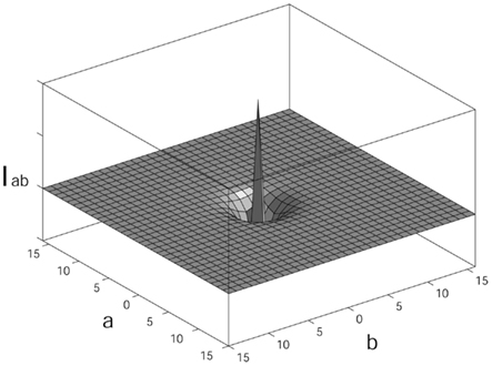
Figure 10. Contrast-enhancing filter, which has the effect of local lateral inhibition. The parameters δ and σ are variables used in equation (5) to modify the amount and extent of inhibition, respectively.

$I_{a,b}=\left\{\begin{array}{cc}-\delta e^{-\frac{a^2+b^2}{{\sigma }^2}}\hfill & \text{if}a\ne 0\text{or}b\ne 0,\hfill \\ 1-\sum _{a\ne 0,b\ne 0}{I}_{a,b}\hfill & \text{if}a=0\text{and}b=0.\hfill \\ \hfill \end{array}\right.$ (5)

This is a filter that leaves the average activity unchanged. A modified version of this filter designed as a difference of Gaussians with the same inhibition but shorter range local excitation is being tested to investigate whether the self-organizing maps that this promotes (Rolls, 2008b) helps the system to provide some continuity in the representations formed. The concept is that this may help the system to code efficiently for large numbers of untrained stimuli that fall between trained stimuli in similarity space.

The second stage involves contrast enhancement. In VisNet (Wallis and Rolls, 1997), this was implemented by raising the neuronal activations to a fixed power and normalizing the resulting firing within a layer to have an average firing rate equal to 1.0. In VisNet2 (Rolls and Milward, 2000) and in subsequent simulations a more biologically plausible form of the activation function, a sigmoid, was used:

$y={\text{f}}^{\text{sigmoid}}\left(r\right)=\frac{1}{1+e^{-2\beta \left(r-\alpha \right)}}$ (6)

where r is the activation (or firing rate) of the neuron after the lateral inhibition, y is the firing rate after the contrast enhancement produced by the activation function, and β is the slope or gain and α is the threshold or bias of the activation function. The sigmoid bounds the firing rate between 0 and 1 so global normalization is not required. The slope and threshold are held constant within each layer. The slope is constant throughout training, whereas the threshold is used to control the sparseness of firing rates within each layer. The (population) sparseness of the firing within a layer is defined (Rolls and Treves, 1998, 2011; Franco et al., 2007; Rolls, 2008b) as:

$a=\frac{{\left({\displaystyle {\sum }_i{y}_i}/n\right)}^2}{{\displaystyle {\sum }_i{y}_i^2}/n}$ (7)

where n is the number of neurons in the layer. To set the sparseness to a given value, e.g., 5%, the threshold is set to the value of the 95th percentile point of the activations within the layer. (Unless otherwise stated here, the neurons used the sigmoid activation function as just described.)

In most simulations with VisNet2 and later, the sigmoid activation function was used with parameters (selected after a number of optimization runs) as shown in Table 2.

TABLE 2

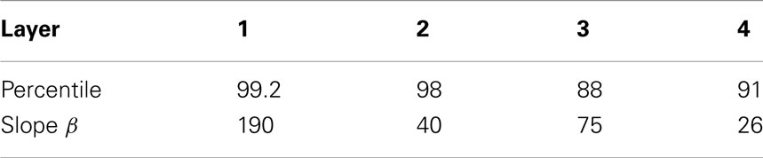
Table 2. Sigmoid parameters for the runs with 25 locations by Rolls and Milward, 2000).

In addition, the lateral inhibition parameters normally used in VisNet2 simulations are as shown in Table 3. (Where a power activation function was used in the simulations of Wallis and Rolls (1997), the power for layer 1 was 6, and for the other layers was 2.)

TABLE 3

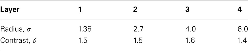
Table 3. Lateral inhibition parameters for the 25-location runs.

5.1.4. The input to VisNet

VisNet is provided with a set of input filters which can be applied to an image to produce inputs to the network which correspond to those provided by simple cells in visual cortical area 1 (V1). The purpose of this is to enable within VisNet the more complicated response properties of cells between V1 and the inferior temporal cortex (IT) to be investigated, using as inputs natural stimuli such as those that could be applied to the retina of the real visual system. This is to facilitate comparisons between the activity of neurons in VisNet and those in the real visual system, to the same stimuli. In VisNet no attempt is made to train the response properties of simple cells, but instead we start with a defined series of filters to perform fixed feature extraction to a level equivalent to that of simple cells in V1, as have other researchers in the field (Fukushima, 1980; Buhmann et al., 1991; Hummel and Biederman, 1992), because we wish to simulate the more complicated response properties of cells between V1 and the inferior temporal cortex (IT). The elongated orientation-tuned input filters used accord with the general tuning profiles of simple cells in V1 (Hawken and Parker, 1987) and in earlier versions of VisNet were computed by weighting the difference of two Gaussians by a third orthogonal Gaussian as described in detail elsewhere (Wallis and Rolls, 1997; Rolls and Milward, 2000; Perry et al., 2010). Each individual filter is tuned to spatial-frequency (0.0039–0.5 cycles/pixel over eight octaves); orientation (0–135° in steps of 45°); and sign (±1). Of the 272 layer 1 connections, the number to each group in VisNetL is as shown in Table 4. In VisNet2 (Rolls and Milward, 2000; used for most VisNet simulations) only even symmetric – “bar detecting” – filter shapes are used, which take the form of a Gaussian shape along the axis of orientation tuning for the filter, and a difference of Gaussians along the perpendicular axis.

TABLE 4

Table 4. VisNet layer 1 connectivity.

This filter is referred to as an oriented difference of Gaussians, or DOG filter. Any zero D.C. filter can of course produce a negative as well as positive output, which would mean that this simulation of a simple cell would permit negative as well as positive firing. In contrast to some other models the response of each filter is zero thresholded and the negative results used to form a separate anti-phase input to the network. The filter outputs are also normalized across scales to compensate for the low-frequency bias in the images of natural objects.

However, Gabor filters have also been tested, also produce good results with VisNet (Deco and Rolls, 2004), and are what we implement at present in VisNetL. Following Daugman (1988) the receptive fields of the simple cell-like input neurons are modeled by 2D-Gabor functions. The Gabor receptive fields have five degrees of freedom given essentially by the product of an elliptical Gaussian and a complex plane wave. The first two degrees of freedom are the 2D-locations of the receptive field’s center; the third is the size of the receptive field; the fourth is the orientation of the boundaries separating excitatory and inhibitory regions; and the fifth is the symmetry. This fifth degree of freedom is given in the standard Gabor transform by the real and imaginary part, i.e., by the phase of the complex function representing it, whereas in a biological context this can be done by combining pairs of neurons with even and odd receptive fields. This design is supported by the experimental work of Pollen and Ronner (1981), who found simple cells in quadrature-phase pairs. Even more, Daugman (1988) proposed that an ensemble of simple cells is best modeled as a family of 2D-Gabor wavelets sampling the frequency domain in a log-polar manner as a function of eccentricity. Experimental neurophysiological evidence constrains the relation between the free parameters that define a 2D-Gabor receptive field (De Valois and De Valois, 1988). There are three constraints fixing the relation between the width, height, orientation, and spatial-frequency (Lee, 1996). The first constraint posits that the aspect ratio of the elliptical Gaussian envelope is 2:1. The second constraint postulates that the plane wave tends to have its propagating direction along the short axis of the elliptical Gaussian. The third constraint assumes that the half-amplitude bandwidth of the frequency response is about 1–1.5 octaves along the optimal orientation. Further, we assume that the mean is zero in order to have an admissible wavelet basis (Lee, 1996).

In more detail, the Gabor filters are constructed as follows (Deco and Rolls, 2004). We consider a pixelized gray-scale image given by a N × N matrix ${\Gamma }_{ij}^{\text{orig}}.$ The subindices ij denote the spatial position of the pixel. Each pixel value is given a gray-level brightness value coded in a scale between 0 (black) and 255 (white). The first step in the pre-processing consists of removing the DC component of the image (i.e., the mean value of the gray-scale intensity of the pixels). (The equivalent in the brain is the low-pass filtering performed by the retinal ganglion cells and lateral geniculate cells. The visual representation in the LGN is essentially a contrast-invariant pixel representation of the image, i.e., each neuron encodes the relative brightness value at one location in visual space referred to the mean value of the image brightness.) We denote this contrast-invariant LGN representation by the N × N matrix ${\Gamma }_{ij}$ defined by the equation

${\Gamma }_{ij}={\Gamma }_{ij}^{\text{orig}}-\frac{1}{N^2}\sum _{i=1}^N\sum _{j=1}^N{\Gamma }_{ij}^{\text{orig}}.$ (8)

Feed-forward connections to a layer of V1 neurons perform the extraction of simple features like bars at different locations, orientations and sizes. Realistic receptive fields for V1 neurons that extract these simple features can be represented by 2D-Gabor wavelets. Lee (1996) derived a family of discretized 2D-Gabor wavelets that satisfy the wavelet theory and the neurophysiological constraints for simple cells mentioned above. They are given by an expression of the form

$G_{pqkl}\left(x,y\right)=a^{-k}{\Psi }_{{\Theta }_l}\left(a^{-k}\left(x-2p\right),a^{-k}\left(y-2q\right)\right)$ (9)

where

${\Psi }_{{\Theta }_l}=\Psi \left(xcos\left(l{\Theta }_0\right)+ysin\left(l{\Theta }_0\right),-xsin\left(l{\Theta }_0\right)+ycos\left(l{\Theta }_0\right)\right),$ (10)

and the mother wavelet is given by

$\Psi \left(x,y\right)=\frac{1}{\sqrt{2\pi }}{e}^{-\frac{1}{8}\left(4x^2+y^2\right)}\left[e^{i\kappa x}-e^{-\frac{{\kappa }^2}{2}}\right].$ (11)

In the above equations Θ₀ = π/L denotes the step size of each angular rotation; l the index of rotation corresponding to the preferred orientation Θ_l = lπ/L; k denotes the octave; and the indices pq the position of the receptive field center at c_x = p and c_y = q. In this form, the receptive fields at all levels cover the spatial domain in the same way, i.e., by always overlapping the receptive fields in the same fashion. In the model we use a = 2, b = 1, and κ = π corresponding to a spatial-frequency bandwidth of one octave. We now use in VisNetL both symmetric and asymmetric filters (as both are present in V1 Ringach, 2002); with the angular spacing between the different orientations set to 45°; and with 8 filter frequencies spaced one octave apart starting with 0.5 cycles per pixel, and with the sampling from the spatial frequencies set as shown in Table 4.

Cells of layer 1 receive a topologically consistent, localized, random selection of the filter responses in the input layer, under the constraint that each cell samples every filter spatial-frequency and receives a constant number of inputs. Figure 11 shows pictorially the general filter sampling paradigm.

FIGURE 11

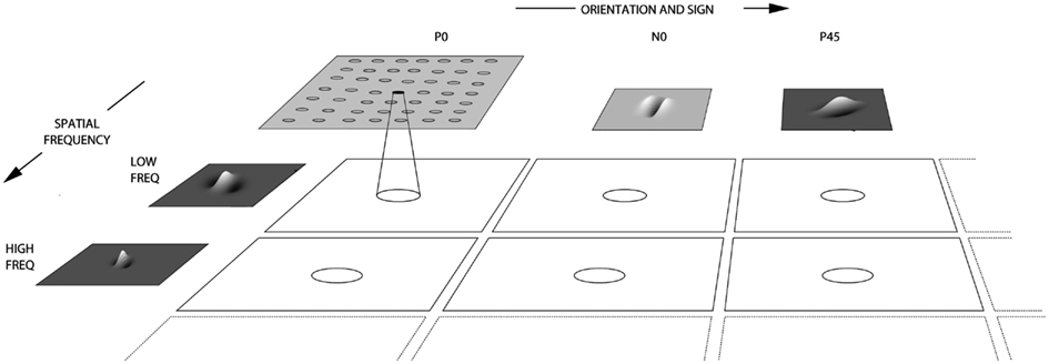
Figure 11. The filter sampling paradigm. Here each square represents the retinal image presented to the network after being filtered by a Gabor filter of the appropriate orientation sign and frequency. The circles represent the consistent retinotopic coordinates used to provide input to a layer 1 cell. The filters double in spatial-frequency toward the reader. Left to right the orientation tuning increases from 0° in steps of 45°, with segregated pairs of positive (P) and negative (N) filter responses.

5.1.5. Measures for network performance

A neuron can be said to have learnt an invariant representation if it discriminates one set of stimuli from another set, across all transformations. For example, a neuron’s response is translation-invariant if its response to one set of stimuli irrespective of presentation is consistently higher than for all other stimuli irrespective of presentation location. Note that we state “set of stimuli” since neurons in the inferior temporal cortex are not generally selective for a single stimulus but rather a subpopulation of stimuli (Baylis et al., 1985; Abbott et al., 1996; Rolls et al., 1997b; Rolls and Treves, 1998, 2011; Rolls and Deco, 2002; Franco et al., 2007; Rolls, 2007b, 2008b). The measure of network performance used in VisNet1 (Wallis and Rolls, 1997), the “Fisher metric” (referred to in some figure labels as the Discrimination Factor), reflects how well a neuron discriminates between stimuli, compared to how well it discriminates between different locations (or more generally the images used rather than the objects, each of which is represented by a set of images, over which invariant stimulus or object representations must be learned). The Fisher measure is very similar to taking the ratio of the two F values in a two-way ANOVA, where one factor is the stimulus shown, and the other factor is the position in which a stimulus is shown. The measure takes a value greater than 1.0 if a neuron has more different responses to the stimuli than to the locations. That is, values greater than 1 indicate invariant representations when this measure is used in the following figures. Further details of how the measure is calculated are given by Wallis and Rolls (1997).

Measures of network performance based on information theory and similar to those used in the analysis of the firing of real neurons in the brain (Rolls, 2008b; Rolls and Treves, 2011) were introduced by Rolls and Milward (2000) for VisNet2, and are used in later papers. A single cell information measure was introduced which is the maximum amount of information the cell has about any one stimulus/object independently of which transform (e.g., position on the retina) is shown. Because the competitive algorithm used in VisNet tends to produce local representations (in which single cells become tuned to one stimulus or object), this information measure can approach log₂ N_s bits, where N_s is the number of different stimuli. Indeed, it is an advantage of this measure that it has a defined maximal value, which enables how well the network is performing to be quantified. Rolls and Milward (2000) showed that the Fisher and single cell information measures were highly correlated, and given the advantage just noted of the information measure, it was adopted in Rolls and Milward (2000) and subsequent papers. Rolls and Milward (2000) also introduced a multiple cell information measure, which has the advantage that it provides a measure of whether all stimuli are encoded by different neurons in the network. Again, a high value of this measure indicates good performance.

For completeness, we provide further specification of the two information theoretic measures, which are described in detail by Rolls and Milward (2000), (see Rolls, 2008b) Rolls and Treves (2011) for an introduction to the concepts). The measures assess the extent to which either a single cell, or a population of cells, responds to the same stimulus invariantly with respect to its location, yet responds differently to different stimuli. The measures effectively show what one learns about which stimulus was presented from a single presentation of the stimulus at any randomly chosen location. Results for top (4th) layer cells are shown. High information measures thus show that cells fire similarly to the different transforms of a given stimulus (object), and differently to the other stimuli. The single cell stimulus-specific information, I(s, R), is the amount of information the set of responses, R, has about a specific stimulus, s (see Rolls et al., 1997c; Rolls and Milward, 2000). I(s, R) is given by

$I\left(s,R\right)=\sum _{r\in R}P\left(r|s\right){log}_2\frac{P\left(r|s\right)}{P\left(r\right)}$ (12)

where r is an individual response from the set of responses R of the neuron. For each cell the performance measure used was the maximum amount of information a cell conveyed about any one stimulus. This (rather than the mutual information, I(S, R) where S is the whole set of stimuli s), is appropriate for a competitive network in which the cells tend to become tuned to one stimulus. (I(s, R) has more recently been called the stimulus-specific surprise (DeWeese and Meister, 1999; Rolls and Treves, 2011). Its average across stimuli is the mutual information I(S, R).)

If all the output cells of VisNet learned to respond to the same stimulus, then the information about the set of stimuli S would be very poor, and would not reach its maximal value of log₂ of the number of stimuli (in bits). The second measure that is used here is the information provided by a set of cells about the stimulus set, using the procedures described by Rolls et al. (1997b) and Rolls and Milward (2000). The multiple cell information is the mutual information between the whole set of stimuli S and of responses R calculated using a decoding procedure in which the stimulus s′ that gave rise to the particular firing rate response vector on each trial is estimated. (The decoding step is needed because the high dimensionality of the response space would lead to an inaccurate estimate of the information if the responses were used directly, as described by Rolls et al. (1997b) and Rolls and Treves (1998).) A probability table is then constructed of the real stimuli s and the decoded stimuli s′. From this probability table, the mutual information between the set of actual stimuli S and the decoded estimates S′ is calculated as

$I\left(S,S^{\prime }\right)=\sum _{s,s^{\prime }}P\left(s,s^{\prime }\right){log}_2\frac{P\left(s,s^{\prime }\right)}{P\left(s\right)P\left(s^{\prime }\right)}$ (13)

This was calculated for the subset of cells which had as single cells the most information about which stimulus was shown. In particular, in Rolls and Milward (2000) and subsequent papers, the multiple cell information was calculated from the first five cells for each stimulus that had maximal single cell information about that stimulus, that is from a population of 35 cells if there were seven stimuli (each of which might have been shown in, for example, 9 or 25 positions on the retina).

5.2. Initial Experiments with VisNet

Having established a network model, Wallis and Rolls (1997) following a first report by Wallis et al. (1993) described four experiments in which the theory of how invariant representations could be formed was tested using a variety of stimuli undergoing a number of natural transformations. In each case the network produced neurons in the final layer whose responses were largely invariant across a transformation and highly discriminating between stimuli or sets of stimuli. A summary showing how the network performed is presented here, with much more evidence of the factors that influence the network’s performance described elsewhere (Wallis and Rolls, 1997; Rolls, 2008b).

5.2.1. “T,” “L,” and “+” as stimuli: learning translation invariance

One of the classical properties of inferior temporal cortex face cells is their invariant response to face stimuli translated across the visual field (Tovee et al., 1994). In this first experiment, the learning of translation-invariant representations by VisNet was investigated.

In order to test the network a set of three stimuli, based upon probable 3D edge cues – consisting of a “T,” “L,” and “+” shape – was constructed. Chakravarty (1979) describes the application of these shapes as cues for the 3D interpretation of edge junctions, and Tanaka et al. (1991) have demonstrated the existence of cells responsive to such stimuli in IT.) These stimuli were chosen partly because of their significance as form cues, but on a more practical note because they each contain the same fundamental features – namely a horizontal bar conjoined with a vertical bar. In practice this means that the oriented simple cell filters of the input layer cannot distinguish these stimuli on the basis of which features are present. As a consequence of this, the representation of the stimuli received by the network is non-orthogonal and hence considerably more difficult to classify than was the case in earlier experiments involving the trace rule described by Földiák (1991). The expectation is that layer 1 neurons would learn to respond to spatially selective combinations of the basic features thereby helping to distinguish these non-orthogonal stimuli. The trajectory followed by each stimulus consisted of sweeping left to right horizontally across three locations in the top row, and then sweeping back, right to left across the middle row, before returning to the right hand side across the bottom row – tracing out a “Z” shape path across the retina. Unless stated otherwise this pattern of nine presentation locations was adopted in all image translation experiments described by Wallis and Rolls (1997).

Training was carried out by permutatively presenting all stimuli in each location a total of 800 times. The sequence described above was followed for each stimulus, with the sequence start point and direction of sweep being chosen at random for each of the 800 training trials.

Figures 12 and 13 shows the response after training of a first layer neuron selective for the “T” stimulus. The weighted sum of all filter inputs reveals the combination of horizontally and vertically tuned filters in identifying the stimulus. In this case many connections to the lower frequency filters have been reduced to zero by the learning process, except at the relevant orientations. This contrasts strongly with the random wiring present before training (Wallis and Rolls, 1997; Rolls, 2008b). It is important that neurons at early stages of feature hierarchy networks respond to combinations of features in defined relative spatial positions, before invariance is built into the system, as this is part of the way that the binding problem is solved, as described in more detail in Section 5.4 and by Elliffe et al. (2002). The feature combination tuning is illustrated by the VisNet layer 1 neuron shown in Figures 12 and 13.

FIGURE 12

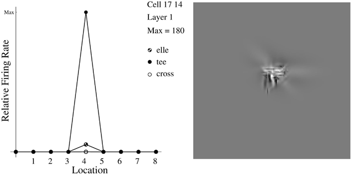
Figure 12. The left graph shows the response of a layer 1 neuron to the three training stimuli for the nine training locations. Alongside this are the results of summating all the filter inputs to the neuron. The discrimination factor for this cell was 1.04.

FIGURE 13

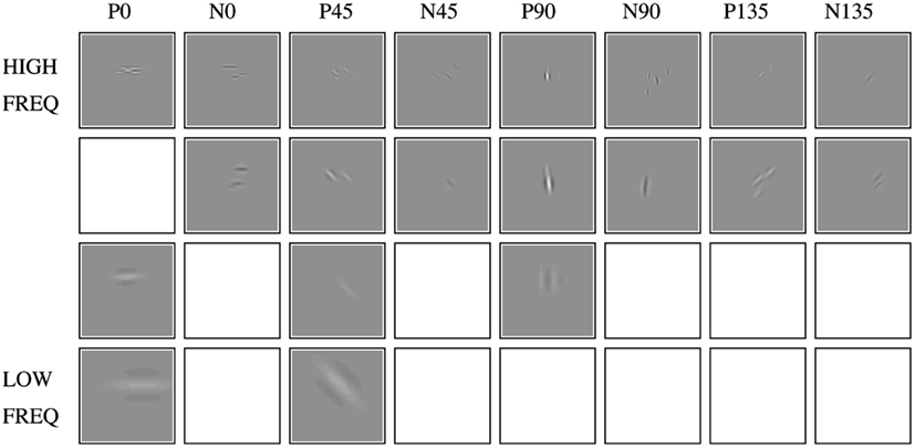
Figure 13. The connections to a single cell in layer 1 of VisNet from the filters after training in the T, L, and + stimulus set, represented by plotting the receptive fields of every input layer cell connected to the particular layer 1 cell. Separate input layer cells have activity that represents a positive (P) or negative (N) output from the bank of filters which have different orientations in degrees (the columns) and different spatial frequencies (the rows). Here the overall receptive field of the layer 1 cell is centered just below the center-point of the retina. The connection scheme allows for relatively fewer connections to lower frequency cells than to high-frequency cells in order to cover a similar region of the input at each frequency. The blank squares indicate that no connection exists between the layer 1 cell chosen and the filters of that particular orientation, sign, and spatial-frequency.

The results for layer 4 neurons are illustrated in Figure 14. By this stage translation-invariant, stimulus-identifying, cells have emerged. The response profiles confirm the high level of neural selectivity for a particular stimulus irrespective of location. Neurons in layers 2 and 3 of VisNet had intermediate-levels of translation invariance to those illustrated for layer 1 and layer 4. The gradual increase in the invariance that the tolerance to shifts of the preferred stimulus gradually builds up through the layers.

FIGURE 14

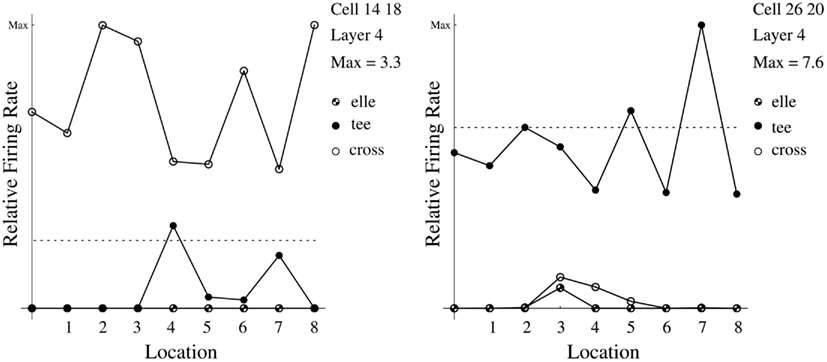
Figure 14. Response profiles for two fourth layer neurons – discrimination factors 4.07 and 3.62 – in the L, T, and + experiment.

The trace used in VisNet enables successive features that, based on the natural statistics of the visual input, are likely to be from the same object or feature complex to be associated together. For good performance, the temporal trace needs to be sufficiently long that it covers the period in which features seen by a particular neuron in the hierarchy are likely to come from the same object. On the other hand, the trace should not be so long that it produces associations between features that are parts of different objects, seen when, for example, the eyes move to another object. One possibility is to reset the trace during saccades between different objects. If explicit trace resetting is not implemented, then the trace should, to optimize the compromise implied by the above, lead to strong associations between temporally close stimuli, and increasingly weaker associations between temporally more distant stimuli. In fact, the trace implemented in VisNet has an exponential decay, and it has been shown that this form is optimal in the situation where the exact duration over which the same object is being viewed varies, and where the natural statistics of the visual input happen also to show a decreasing probability that the same object is being viewed as the time period in question increases (Wallis and Baddeley, 1997). Moreover, performance can be enhanced if the duration of the trace does at the same time approximately match the period over which the input stimuli are likely to come from the same object or feature complex (Wallis and Rolls, 1997; Rolls, 2008b). Nevertheless, good performance can be obtained in conditions under which the trace rule allows associations to be formed only between successive items in the visual stream (Rolls and Milward, 2000; Rolls and Stringer, 2001).

It is also the case that the optimal value of η in the trace rule is likely to be different for different layers of VisNet, and for cortical processing in the “what” visual stream. For early layers of the system, small movements of the eyes might lead to different feature combinations providing the input to cells (which at early stages have small receptive fields), and a short duration of the trace would be optimal. However, these small eye movements might be around the same object, and later layers of the architecture would benefit from being able to associate together their inputs over longer times, in order to learn about the larger scale properties that characterize individual objects, including, for example, different views of objects observed as an object turns or is turned. Thus the suggestion is made that the temporal trace could be effectively longer at later stages (e.g., inferior temporal visual cortex) compared to early stages (e.g., V2 and V4) of processing in the visual system. In addition, as will be shown in Section 5.4, it is important to form feature combinations with high-spatial precision before invariance learning supported by a temporal trace starts, in order that the feature combinations and not the individual features have invariant representations. This leads to the suggestion that the trace rule should either not operate, or be short, at early stages of cortical visual processing such as V1. This is reflected in the operation of VisNet2, which does not use a temporal trace in layer 1 (Rolls and Milward, 2000).

5.2.2. Faces as stimuli: translation invariance

The aim of the next set of experiments described by Wallis and Rolls (1997) was to start to address the issues of how the network operates when invariant representations must be learned for a larger number of stimuli, and whether the network can learn when much more complicated, real biological stimuli, faces, are used.

Figure 15 contrasts the measure of invariance, or discrimination factor, achieved by cells in the four layers, averaged over five separate runs of the network (Wallis and Rolls, 1997; Rolls, 2008b). Translation invariance clearly increases through the layers, as expected.

FIGURE 15

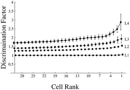
Figure 15. Variation in network performance for the top 30 most highly discriminating cells through the four layers of the network, averaged over five runs of the network. The net was trained on 7 faces each in 9 locations.

Having established that invariant cells have emerged in the final layer, we now consider the role of the trace rule, by assessing the network tested under two new conditions. Firstly, the performance of the network was measured before learning occurs, that is with its initially random connection weights. Secondly, the network was trained with η in the trace rule set to 0, which causes learning to proceed in a traceless, standard Hebbian, fashion. (Hebbian learning is purely associative Rolls, 2008b.) Figure 16 shows the results under the three training conditions. The results show that the trace rule is the decisive factor in establishing the invariant responses in the layer 4 neurons. It is interesting to note that the Hebbian learning results are actually worse than those achieved by chance in the untrained net. In general, with Hebbian learning, the most highly discriminating cells barely rate higher than 1. This value of discrimination corresponds to the case in which a cell responds to only one stimulus and in only one location. The poor performance with the Hebb rule comes as a direct consequence of the presentation paradigm being employed. If we consider an image as representing a vector in multidimensional space, a particular image in the top left-hand corner of the input retina will tend to look more like any other image in that same location than the same image presented elsewhere. A simple competitive network using just Hebbian learning will thus tend to categorize images by where they are rather than what they are – the exact opposite of what the net was intended to learn. This comparison thus indicates that a small memory trace acting in the standard Hebbian learning paradigm can radically alter the normal vector averaging, image classification, performed by a Hebbian-based competitive network.

FIGURE 16

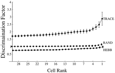
Figure 16. Variation in network performance for the top 30 most highly discriminating cells in the fourth layer for the three training regimes, averaged over five runs of the network. The net was trained on 7 faces each in 9 locations.

In order to check that there was an invariant representation in layer 4 of VisNet that could be read by a receiving population of neurons, a fifth layer was added to the net which fully sampled the fourth layer cells. This layer was in turn trained in a supervised manner using gradient descent or with a Hebbian associative learning rule. (Wallis and Rolls, 1997) showed that the object classification performed by the layer 5 network was better if the network had been trained with the trace rule than when it was untrained or was trained with a Hebb rule.

5.2.3. Faces as stimuli: view-invariance

Given that the network had been shown to be able to operate usefully with a more difficult translation invariance problem, we next addressed the question of whether the network can solve other types of transform invariance, as we had intended. The next experiment addressed this question, by training the network on the problem of 3D stimulus rotation, which produces non-isomorphic transforms, to determine whether the network can build a view-invariant categorization of the stimuli (Wallis and Rolls, 1997). The trace rule learning paradigm should, in conjunction with the architecture described here, prove capable of learning any of the transforms tolerated by IT neurons, so long as each stimulus is presented in short sequences during which the transformation occurs and can be learned. This experiment continued with the use of faces but now presented them centrally in the retina in a sequence of different views of a face (Wallis and Rolls, 1997; Rolls, 2008b). The faces were again smoothed at the edges to erase the harsh image boundaries, and the D.C. term was removed. During the 800 epochs of learning, each stimulus was chosen at random, and a sequence of preset views of it was shown, rotating the face either to the left or to the right.

Although the actual number of images being presented is smaller, some 21 views in all, there is good reason to think that this problem may be harder to solve than the previous translation experiments. This is simply due to the fact that all 21 views exactly overlap with one another. The net was indeed able to solve the invariance problem, with examples of invariant layer 4 neuron response profiles appearing in Figure 17.

FIGURE 17

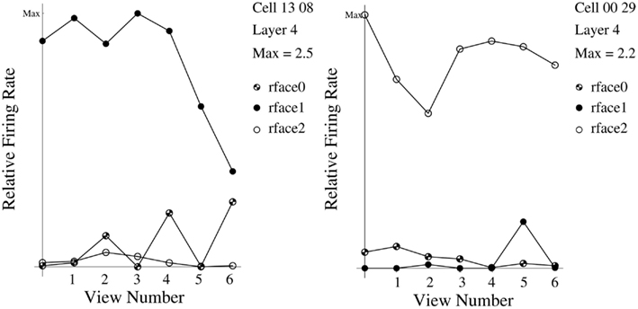
Figure 17. Response profiles for cells in the last two layers of the network – discrimination factors 11.12 and 12.40 – in the experiment with seven different views of each of three faces.

Further analyses confirmed the good performance on view-invariance learning (Wallis and Rolls, 1997; Rolls, 2008b).

5.3. Different Forms of the Trace-Learning Rule, and Their Relation to Error Correction and Temporal Difference Learning

The original trace-learning rule used in the simulations of Wallis and Rolls (1997) took the form

$\delta w_j=\alpha {ȳ}^{\tau }{x}_j^{\tau }$ (14)

where the trace ${ȳ}^{\tau }$ is updated according to

${\overline{y}}^{\tau }=\left(1-\eta \right)y^{\tau }+\eta {\overline{y}}^{\tau -1}.$ (15)

The parameter η ∈ [0, 1] controls the relative contributions to the trace ${ȳ}^{\tau }$ from the instantaneous firing rate y^τ and the trace at the previous time step ${ȳ}^{\tau -1},$ where for η = 0 we have ${ȳ}^{\tau }=y^{\tau }$ and equation (14) becomes the standard Hebb rule

$\delta w_j=\alpha y^{\tau }{x}_j^{\tau }.$ (16)

At the start of a series of investigations of different forms of the trace-learning rule (Rolls and Milward, 2000) demonstrated that VisNet’s performance could be greatly enhanced (see Figure 18) with a modified Hebbian trace-learning rule (equation (17)) that incorporated a trace of activity from the preceding time steps, with no contribution from the activity being produced by the stimulus at the current time step. This rule took the form

FIGURE 18

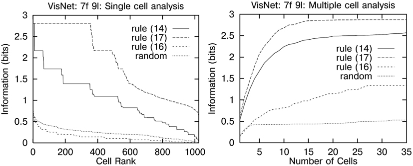
Figure 18. Numerical results with the standard trace rule (14), the modified trace-learning rule (17), the Hebb rule (16), and random weights, trained on 7 faces in 9 locations: single cell information measure (left), multiple cell information measure (right). (After Rolls and Stringer, 2001a.)

$\delta w_j=\alpha {\overline{y}}^{\tau -1}{x}_j^x.$ (17)

The trace shown in equation (17) is in the post-synaptic term, and similar effects were found if the trace was in the presynaptic term, or in both the pre- and the post-synaptic terms. The crucial difference from the earlier rule (see equation (14)) was that the trace should be calculated up to only the preceding timestep, with no contribution to the trace from the firing on the current trial to the current stimulus. How might this be understood?

One way to understand this is to note that the trace rule is trying to set up the synaptic weight on trial τ based on whether the neuron, based on its previous history, is responding to that stimulus (in other transforms, e.g., position). Use of the trace rule at τ − 1 does this that is it takes into account the firing of the neuron on previous trials, with no contribution from the firing being produced by the stimulus on the current trial. On the other hand, use of the trace at time τ in the update takes into account the current firing of the neuron to the stimulus in that particular position, which is not a good estimate of whether that neuron should be allocated to invariantly represent that stimulus. Effectively, using the trace at time τ introduces a Hebbian element into the update, which tends to build position-encoded analyzers, rather than stimulus-encoded analyzers. (The argument has been phrased for a system learning translation invariance, but applies to the learning of all types of invariance.) A particular advantage of using the trace at τ − 1 is that the trace will then on different occasions (due to the randomness in the location sequences used) reflect previous histories with different sets of positions, enabling the learning of the neuron to be based on evidence from the stimulus present in many different positions. Using a term from the current firing in the trace (i.e., the trace calculated at time τ) results in this desirable effect always having an undesirable element from the current firing of the neuron to the stimulus in its current position.

5.3.1. The modified Hebbian trace rule and its relation to error correction

The rule of equation (17) corrects the weights using a post-synaptic trace obtained from the previous firing (produced by other transforms of the same stimulus), with no contribution to the trace from the current post-synaptic firing (produced by the current transform of the stimulus). Indeed, insofar as the current firing y^τ is not the same as ${ȳ}^{\tau -1},$ this difference can be thought of as an error. This leads to a conceptualization of using the difference between the current firing and the preceding trace as an error correction term, as noted in the context of modeling the temporal properties of classical conditioning by Sutton and Barto (1981), and developed next in the context of invariance learning (see Rolls and Stringer, 2001).

First, we re-express the rule of equation (17) in an alternative form as follows. Suppose we are at timestep τ and have just calculated a neuronal firing rate y^τ and the corresponding trace ${ȳ}^{\tau }$ from the trace update equation (15). If we assume η ∈ (0, 1), then rearranging equation (15) gives

${\overline{y}}^{\tau -1}=\frac{1}{\eta }\left({\overline{y}}^{\tau }-\left(1-\eta \right)y^{\tau }\right),$ (18)

and substituting equation (18) into equation (17) gives

$\begin{array}{l}\delta w_j=\alpha \frac{1}{\eta }\left({\overline{y}}^{\tau }-\left(1-\eta \right)y^{\tau }\right)x_j^{\tau }\\ =\alpha \frac{1-\eta }{\eta }\left(\frac{1}{1-\eta }{\overline{y}}^{\tau }-y^{\tau }\right)x_j^{\tau }\\ =\widehat{\alpha }\left(\widehat{\beta }{\overline{y}}^{\tau }-y^{\tau }\right)x_j^{\tau }\end{array}$ (19)

where $\widehat{\alpha }=\alpha \frac{1-\eta }{\eta }$ and $\widehat{\beta }=\frac{1}{1-\eta }.$ The modified Hebbian trace-learning rule (17) is thus equivalent to equation (19) which is in the general form of an error correction rule (Hertz et al., 1991). That is, rule (19) involves the subtraction of the current firing rate y^τ from a target value, in this case $\widehat{\beta }{ȳ}^{\tau }.$

Although above we have referred to rule (17) as a modified Hebbian rule, we note that it is only associative in the sense of associating previous cell firing with the current cell inputs. In the next section we continue to explore the error correction paradigm, examining five alternative examples of this sort of learning rule.

5.3.2. Five forms of error correction learning rule

Error correction learning rules are derived from gradient descent minimization (Hertz et al., 1991), and continually compare the current neuronal output to a target value t and adjust the synaptic weights according to the following equation at a particular timestep τ

$\delta w_j=\alpha \left(t-y^{\tau }\right)x_j^{\tau }.$ (20)

In this usual form of gradient descent by error correction, the target t is fixed. However, in keeping with our aim of encouraging neurons to respond similarly to images that occur close together in time it seems reasonable to set the target at a particular timestep, t^τ, to be some function of cell activity occurring close in time, because encouraging neurons to respond to temporal classes will tend to make them respond to the different variants of a given stimulus (Földiák, 1991; Rolls, 1992; Wallis and Rolls, 1997). For this reason, Rolls and Stringer (2001) explored a range of error correction rules where the targets t^τ are based on the trace of neuronal activity calculated according to equation (15). We note that although the target is not a fixed value as in standard error correction learning, nevertheless the new learning rules perform gradient descent on each timestep, as elaborated below. Although the target may be varying early on in learning, as learning proceeds the target is expected to become more and more constant, as neurons settle to respond invariantly to particular stimuli. The first set of five error correction rules we discuss are as follows.

$\begin{array}{rcll}\delta w_j& =\alpha \left(\beta {ȳ}^{\tau -1}-y^{\tau }\right)x_j^{\tau },& & \text{(21)}\\ \delta w_j& =\alpha \left(\beta y^{\tau -1}-y^{\tau }\right)x_j^{\tau },& & \text{(22)}\\ \delta w_j& =\alpha \left(\beta {ȳ}^{\tau }-y^{\tau }\right)x_j^{\tau },& & \text{(23)}\\ \delta w_j& =\alpha \left(\beta {ȳ}^{\tau +1}-y^{\tau }\right)x_j^{\tau },& & \text{(24)}\\ \delta w_j& =\alpha \left(\beta y^{\tau +1}-y^{\tau }\right)x_j^{\tau },& & \text{(25)}\end{array}$

where updates (21–23) are performed at timestep τ, and updates (24) and (25) are performed at timestep τ + 1. (The reason for adopting this convention is that the basic form of the error correction rule (20) is kept, with the five different rules simply replacing the term t.) It may be readily seen that equations (22) and (25) are special cases of equations (21) and (24), respectively, with η = 0.

These rules are all similar except for their targets t^τ, which are all functions of a temporally nearby value of cell activity. In particular, rule (23) is directly related to rule (19), but is more general in that the parameter $\widehat{\beta }=\frac{1}{1-\eta }$ is replaced by an unconstrained parameter β. In addition, we also note that rule (21) is closely related to a rule developed in Peng et al. (1998) for view-invariance learning. The above five error correction rules are biologically plausible in that the targets t^τ are all local cell variables (see Rolls and Treves, 1998 and Rolls, 2008b). In particular, rule (23) uses the trace ${ȳ}^{\tau }$ from the current time level τ, and rules (22) and (25) do not need exponential trace values $\overline{y}$ instead relying only on the instantaneous firing rates at the current and immediately preceding timesteps. However, all five error correction rules involve decrementing of synaptic weights according to an error which is calculated by subtracting the current activity from a target.

Numerical results with the error correction rules trained on 7 faces in 9 locations are presented by Rolls and Stringer (2001). For all the results the synaptic weights were clipped to be positive during the simulation, because it is important to test that decrementing synaptic weights purely within the positive interval w ∈ [0,∞] will provide significantly enhanced performance. That is, it is important to show that error correction rules do not necessarily require possibly biologically implausible modifiable negative weights. For each of the rules (21–25), the parameter β has been individually optimized to the following respective values: 4.9, 2.2, 2.2, 3.8, 2.2. All five error correction rules offer considerably improved performance over both the standard trace rule (14) and rule (17). Networks trained with rule (21) performed best, and this is probably due to two reasons. Firstly, rule (21) incorporates an exponential trace ${ȳ}^{\tau -1}$ in its target t^τ, and we would expect this to help neurons to learn more quickly to respond invariantly to a class of inputs that occur close together in time. Hence, setting η = 0 as in rule (22) results in reduced performance. Secondly, unlike rules (23) and (24), rule (21) does not contain any component of y^τ in its target. If we examine rules (23), (24), we see that their respective targets $\beta {ȳ}^{\tau },$$\beta {ȳ}^{\tau +1}$ contain significant components of y^τ.

5.3.3. Relationship to temporal difference learning

Rolls and Stringer (2001) not only considered the relationship of rule (17) to error correction, but also considered how the error correction rules shown in equations (21–25) are related to temporal difference learning (Sutton, 1988; Sutton and Barto, 1998). Sutton (1988) described temporal difference methods in the context of prediction learning. These methods are a class of incremental learning techniques that can learn to predict final outcomes through comparison of successive predictions from the preceding time steps. This is in contrast to traditional supervised learning, which involves the comparison of predictions only with the final outcome. Consider a series of multistep prediction problems in which for each problem there is a sequence of observation vectors, x¹, x², …, x ^m, at successive timesteps, followed by a final scalar outcome z. For each sequence of observations temporal difference methods form a sequence of predictions y¹, y², …, y^m, each of which is a prediction of z. These predictions are based on the observation vectors x^τ and a vector of modifiable weights w; i.e., the prediction at time step τ is given by y^τ(x^τ, w), and for a linear dependency the prediction is given by y^τ = w ^T x^τ. (Note here that w ^T is the transpose of the weight vector w.) The problem of prediction is to calculate the weight vector w such that the predictions y^τ are good estimates of the outcome z.

The supervised learning approach to the prediction problem is to form pairs of observation vectors x^τ and outcome z for all time steps, and compute an update to the weights according to the gradient descent equation

$\delta \mathbf{\text{w}}=\alpha \left(z-y^{\tau }\right){\nabla }_{\mathbf{\text{w}}}{y}^{\tau }$ (26)

where α is a learning rate parameter and ∇_w indicates the gradient with respect to the weight vector w. However, this learning procedure requires all calculation to be done at the end of the sequence, once z is known. To remedy this, it is possible to replace method (26) with a temporal difference algorithm that is mathematically equivalent but allows the computational workload to be spread out over the entire sequence of observations. Temporal difference methods are a particular approach to updating the weights based on the values of successive predictions, y^τ, y^τ+1. Sutton (1988) showed that the following temporal difference algorithm is equivalent to method (26)

$\delta w=\alpha \left(y^{\tau +1}-y^{\tau }\right)\sum _{k=1}^{\tau }{\nabla }_{\mathbf{\text{w}}}{y}^k,$ (27)

where y^m+1 ≡ z. However, unlike method (26) this can be computed incrementally at each successive time step since each update depends only on y^τ+1, y^τ and the sum of ∇_w y^k over previous time steps k. The next step taken in Sutton (1988) is to generalize equation (27) to the following final form of temporal difference algorithm, known as “TD(λ)”

$\delta \mathbf{\text{w}}=\alpha \left(y^{\tau +1}-y^{\tau }\right)\sum _{k=1}^{\tau }{\lambda }^{\tau -k}{\nabla }_{\mathbf{\text{w}}}{y}^k$ (28)

where λ ∈ [0, 1] is an adjustable parameter that controls the weighting on the vectors ∇_w y^k. Equation (28) represents a much broader class of learning rules than the more usual gradient descent-based rule (27), which is in fact the special case TD(1).

A further special case of equation (28) is for λ = 0, i.e., TD(0), as follows

$\delta \mathbf{\text{w}}=\alpha \left(y^{\tau +1}-y^{\tau }\right){\nabla }_{\mathbf{\text{w}}}{y}^{\tau }.$ (29)

But for problems where y^τ is a linear function of x^τ and w, we have ∇_w y^τ = x^τ, and so equation (29) becomes

$\delta \mathbf{\text{w}}=\alpha \left(y^{\tau +1}-y^{\tau }\right){\mathbf{\text{x}}}^{\tau }.$ (30)

If we assume the prediction process is being performed by a neuron with a vector of inputs x^τ, synaptic weight vector w, and output y^τ = w ^Tx^τ, then we see that the TD(0) algorithm (30) is identical to the error correction rule (25) with β = 1. In understanding this comparison with temporal difference learning, it may be useful to note that the firing at the end of a sequence of the transformed exemplars of a stimulus is effectively the temporal difference target z. This establishes a link to temporal difference learning (Rolls, 2008b). Further, we note that from learning epoch to learning epoch, the target z for a given neuron will gradually settle down to be more and more fixed as learning proceeds.

We now explore in more detail the relation between the error correction rules described above and temporal difference learning. For each sequence of observations with a single outcome the temporal difference method (30), when viewed as an error correction rule, is attempting to adapt the weights such that y^τ+1 = y^τ for all successive pairs of time steps – the same general idea underlying the error correction rules (21–25). Furthermore, in Sutton and Barto (1998), where temporal difference methods are applied to reinforcement learning, the TD(λ) approach is again further generalized by replacing the target y^τ+1 by any weighted average of predictions y from arbitrary future timesteps, e.g., $t^{\tau }=\frac{1}{2}{y}^{\tau +3}+\frac{1}{2}{y}^{\tau +7}$, including an exponentially weighted average extending forward in time. So a more general form of the temporal difference algorithm has the form

$\delta \mathbf{\text{w}}=\alpha \left(t^{\tau }-y^{\tau }\right){\mathbf{\text{x}}}^{\tau },$ (31)

where here the target t^τ is an arbitrary weighted average of the predictions y over future timesteps. Of course, with standard temporal difference methods the target t^τ is always an average over future timesteps k = τ + 1, τ + 2, etc. But in the five error correction rules this is only true for the last exemplar (25). This is because with the problem of prediction, for example, the ultimate target of the predictions y¹,…,y^m is a final outcome y^m+1≡z. However, this restriction does not apply to our particular application of neurons trained to respond to temporal classes of inputs within VisNet. Here we only wish to set the firing rates y¹,…,y^m to the same value, not some final given value z. However, the more general error correction rules clearly have a close relationship to standard temporal difference algorithms. For example, it can be seen that equation (22) with β = 1 is in some sense a temporal mirror image of equation (30), particularly if the updates δw_j are added to the weights w_j only at the end of a sequence. That is, rule (22) will attempt to set y¹,…,y^m to an initial value y⁰ ≡ 0. This relationship to temporal difference algorithms allows us to begin to exploit established temporal difference analyses to investigate the convergence properties of the error correction methods (Rolls and Stringer, 2001).

Although the main aim of Rolls and Stringer (2001) in relating error correction rules to temporal difference learning was to begin to exploit established temporal difference analyses, they observed that the most general form of temporal difference learning, TD(λ), in fact suggests an interesting generalization to the existing error correction learning rules for which we currently have λ = 0. Assuming y^τ = w ^Tx^τ and ∇_w y^τ = x^τ, the general equation (28) for TD(λ) becomes

$\delta w=\alpha \left(y^{\tau +1}-y^{\tau }\right)\sum _{k=1}^{\tau }{\lambda }^{\tau -k}{\mathbf{\text{x}}}^k$ (32)

where the term ${\sum }_{k=1}^{\tau }{\lambda }^{\tau -k}{\mathbf{\text{x}}}^k$ is a weighted sum of the vectors x ^k. This suggests generalizing the original five error correction rules (21–25) by replacing the term $x_j^{\tau }$ by a weighted sum ${\widehat{x}}_j^{\tau }={\displaystyle {\sum }_{k=1}^{\tau }{\lambda }^{\tau -k}{x}_j^k}$ with λ ∈ [0, 1]. In Sutton (1988) ${\widehat{x}}_j^{\tau }$ is calculated according to

${\widehat{x}}_j^{\tau }=x_j^{\tau }+\lambda {\widehat{x}}_j^{\tau -1}$ (33)

with ${\widehat{x}}_j^0\equiv 0.$. This gives the following five temporal difference-inspired error correction rules

$\delta w_j=\alpha \left(\beta {\overline{y}}^{\tau -1}-y^{\tau }\right){\widehat{x}}_j^{\tau },$ (34)

$\delta w_j=\alpha \left(\beta y^{\tau -1}-y^{\tau }\right){\widehat{x}}_j^{\tau },$ (35)

$\delta w_j=\alpha \left(\beta {\overline{y}}^{\tau }-y^{\tau }\right){\widehat{x}}_j^{\tau },$ (36)

$\delta w_j=\alpha \left(\beta {\overline{y}}^{\tau +1}-y^{\tau }\right){\widehat{x}}_j^{\tau },$ (37)

$\delta w_j=\alpha \left(\beta y^{\tau +1}-y^{\tau }\right){\widehat{x}}_j^{\tau },$ (38)

where it may be readily seen that equation (35) and (38) are special cases of equations (34) and (37), respectively, with η = 0. As with the trace ${ȳ}^{\tau },$ the term ${\widehat{x}}_j^{\tau }$ is reset to zero when a new stimulus is presented. These five rules can be related to the more general TD(λ) algorithm, but continue to be biologically plausible using only local cell variables. Setting λ = 0 in rules (34–38), gives us back the original error correction rules (21–25) which may now be related to TD(0).

Numerical results with error correction rules (34–38), and ${\widehat{x}}_j^{\tau }$ calculated according to equation (33) with λ = 1, with positive clipping of weights, trained on 7 faces in 9 locations are presented by Rolls and Stringer (2001). For each of the rules (34–38), the parameter β has been individually optimized to the following respective values: 1.7, 1.8, 1.5, 1.6, 1.8. Comparing these five temporal difference-inspired rules it was found that the best performance is obtained with rule (38) where many more cells reach the maximum level of performance possible with respect to the single cell information measure. In fact, this rule offered the best such results. This may well be due to the fact that this rule may be directly compared to the standard TD(1) learning rule, which itself may be related to classical supervised learning for which there are well known optimality results, as discussed further by Rolls and Stringer (2001).

From the simulations described by Rolls and Stringer (2001) it appears that the form of optimization described above associated with TD(1) rather than TD(0) leads to better performance within VisNet. The TD(1)-like rule (38) with λ = 1.0 and β = 1.8 gave considerably superior results to the TD(0)-like rule (25) with β = 2.2. In fact, the former of these two rules provided the best single cell information results in these studies. We hypothesize that these results are related to the fact that only a finite set of image sequences is presented to VisNet, and so the type of optimization performed by TD(1) for repeated presentations of a finite data set is more appropriate for this problem than the form of optimization performed by TD(0).

5.3.4. Discussion of the different training rules

In terms of biological plausibility, we note the following. First, all the learning rules investigated by Rolls and Stringer (2001) are local learning rules, and in this sense are biologically plausible (Rolls and Treves, 1998; Rolls, 2008b). (The rules are local in that the terms used to modify the synaptic weights are potentially available in the pre- and post-synaptic elements.)

Second we note that all the rules do require some evidence of the activity on one or more previous stimulus presentations to be available when the synaptic weights are updated. Some of the rules, e.g., learning rule (23), use the trace ${ȳ}^{\tau }$ from the current time level, while rules (22) and (25) do not need to use an exponential trace of the neuronal firing rate, but only the instantaneous firing rates y at two successive time steps. It is known that synaptic plasticity does involve a combination of separate processes each with potentially differing time courses (Koch, 1999), and these different processes could contribute to trace rule learning. Another mechanism suggested for implementing a trace of previous neuronal activity is the continuing firing for often 300 ms produced by a short (16 ms) presentation of a visual stimulus (Rolls and Tovee, 1994) which is suggested to be implemented by local cortical recurrent attractor networks (Rolls and Treves, 1998).

Third, we note that in utilizing the trace in the targets t^τ, the error correction (or temporal difference-inspired) rules perform a comparison of the instantaneous firing y^τ with a temporally nearby value of the activity, and this comparison involves a subtraction. The subtraction provides an error, which is then used to increase or decrease the synaptic weights. This is a somewhat different operation from long-term depression (LTD) as well as long-term potentiation (LTP), which are associative changes which depend on the pre- and post-synaptic activity. However, it is interesting to note that an error correction rule which appears to involve a subtraction of current firing from a target might be implemented by a combination of an associative process operating with the trace, and an anti-Hebbian process operating to remove the effects of the current firing. For example, the synaptic updates $\delta w_j=\alpha \left(t^{\tau }-y^{\tau }\right)x_j^{\tau }$ can be decomposed into two separate associative processes $\alpha t^{\tau }{x}_j^{\tau }$ and $-\alpha y^{\tau }{x}_j^{\tau },$ that may occur independently. (The target, t^τ, could in this case be just the trace of previous neural activity from the preceding trials, excluding any contribution from the current firing.) Another way to implement an error correction rule using associative synaptic modification would be to force the post-synaptic neuron to respond to the error term. Although this has been postulated to be an effect which could be implemented by the climbing fiber system in the cerebellum (Ito, 1984, 1989; Rolls and Treves, 1998), there is no similar system known for the neocortex, and it is not clear how this particular implementation of error correction might operate in the neocortex.

In Section 5.3.2 we describe five learning rules as error correction rules. We now discuss an interesting difference of these error correction rules from error correction rules as conventionally applied. It is usual to derive the general form of error correction learning rule from gradient descent minimization in the following way (Hertz et al., 1991). Consider the idealized situation of a single neuron with a number of inputs x_j and output $y={\sum }_j{w}_j{x}_j,$ where w_j are the synaptic weights. We assume that there are a number of input patterns and that for the kth input pattern, $x^k={\left[x_1^k,x_2^k,...\right]}^T,$ the output y^k has a target value t^k. Hence an error measure or cost function can be defined as

$e\left(w\right)=\frac{1}{2}\sum _k{\left(t^k-y^k\right)}^2=\frac{1}{2}\sum _k{\left(t^k-\sum _j{w}_j{x}_j^k\right)}^2.$ (39)

This cost function is a function of the input patterns x ^k and the synaptic weight vector w = [w₁, w₂, …]^T. With a fixed set of input patterns, we can reduce the error measure by employing a gradient descent algorithm to calculate an improved set of synaptic weights. Gradient descent achieves this by moving downhill on the error surface defined in w space using the update

$\delta w_j=-\alpha \frac{\partial e}{\partial w_j}=\alpha \sum _k\left(t^k-y^k\right)x_j^k.$ (40)

If we update the weights after each pattern k, then the update takes the form of an error correction rule

$\delta w_j=\alpha \left(t^k-y^k\right)x_j^k,$ (41)

which is also commonly referred to as the delta rule or Widrow–Hoff rule (see Widrow and Hoff, 1960; Widrow and Stearns, 1985). Error correction rules continually compare the neuronal output with its pre-specified target value and adjust the synaptic weights accordingly. In contrast, the way Rolls and Stringer (2001) introduced of utilizing error correction is to specify the target as the activity trace based on the firing rate at nearby timesteps. Now the actual firing at those nearby time steps is not a pre-determined fixed target, but instead depends on how the network has actually evolved. This effectively means the cost function e(w) that is being minimized changes from timestep to timestep. Nevertheless, the concept of calculating an error, and using the magnitude and direction of the error to update the synaptic weights, is the similarity Rolls and Stringer (2001) made to gradient descent learning.

To conclude this discussion, the error correction and temporal difference rules explored by Rolls and Stringer (2001) provide interesting approaches to help understand invariant pattern recognition learning. Although we do not know whether the full power of these rules is expressed in the brain, we provided suggestions about how they might be implemented. At the same time, we note that the original trace rule used by Földiák (1991), Rolls (1992), and Wallis and Rolls (1997) is a simple associative rule, is therefore biologically very plausible, and, while not as powerful as many of the other rules introduced by Rolls and Stringer (2001), can nevertheless solve the same class of problem. Rolls and Stringer (2001) also emphasized that although they demonstrated how a number of new error correction and temporal difference rules might play a role in the context of view-invariant object recognition, they may also operate elsewhere where it is important for neurons to learn to respond similarly to temporal classes of inputs that tend to occur close together in time.

5.4. The Issue of Feature Binding, and a Solution

In this section we investigate two key issues that arise in hierarchical layered network architectures, such as VisNet, other examples of which have been described and analyzed by Fukushima (1980), Ackley et al. (1985), Rosenblatt (1961), and Riesenhuber and Poggio (1999b). One issue is whether the network can discriminate between stimuli that are composed of the same basic alphabet of features. The second issue is whether such network architectures can find solutions to the spatial binding problem. These issues are addressed next and by Elliffe et al. (2002) and Rolls (2008b).

The first issue investigated is whether a hierarchical layered network architecture of the type exemplified by VisNet can discriminate stimuli that are composed of a limited set of features and where the different stimuli include cases where the feature sets are subsets and supersets of those in the other stimuli. An issue is that if the network has learned representations of both the parts and the wholes, will the network identify that the whole is present when it is shown, and not just that one or more parts is present. (In many investigations with VisNet, complex stimuli (such as faces) were used where each stimulus might contain unique features not present in the other stimuli.) To address this issue Elliffe et al. (2002) used stimuli that are composed from a set of four features which are designed so that each feature is spatially separate from the other features, and no unique combination of firing caused, for example, by overlap of horizontal and vertical filter outputs in the input representation distinguishes any one stimulus from the others. The results described in Section 5.4.4 show that VisNet can indeed learn correct invariant representations of stimuli which do consist of feature sets where individual features do not overlap spatially with each other and where the stimuli can be composed of sets of features which are supersets or subsets of those in other stimuli. Fukushima and Miyake (1982) did not address this crucial issue where different stimuli might be composed of subsets or supersets of the same set of features, although they did show that stimuli with partly overlapping features could be discriminated by the Neocognitron.

In Section 5.4.5 we address the spatial binding problem in architectures such as VisNet. This computational problem that needs to be addressed in hierarchical networks such as the primate visual system and VisNet is how representations of features can be (e.g., translation) invariant, yet can specify stimuli or objects in which the features must be specified in the correct spatial arrangement. This is the feature binding problem, discussed, for example, by von der Malsburg (1990), and arising in the context of hierarchical layered systems (Rosenblatt, 1961; Fukushima, 1980; Ackley et al., 1985). The issue is whether or not features are bound into the correct combinations in the correct relative spatial positions, or if alternative combinations of known features or the same features in different relative spatial positions would elicit the same responses. All this has to be achieved while at the same time producing position-invariant recognition of the whole combination of features, that is, the object. This is a major computational issue that needs to be solved for memory systems in the brain to operate correctly. This can be achieved by what is effectively a learning process that builds into the system a set of neurons in the hierarchical network that enables the recognition process to operate correctly with the appropriate position, size, view, etc. invariances.

5.4.1. Syntactic binding of separate neuronal ensembles by synchronization

The problem of syntactic binding of neuronal representations, in which some features must be bound together to form one object, and other simultaneously active features must be bound together to represent another object, has been addressed by von der Malsburg (1990). He has proposed that this could be performed by temporal synchronization of those neurons that were temporarily part of one representation in a different time slot from other neurons that were temporarily part of another representation. The idea is attractive in allowing arbitrary relinking of features in different combinations. Singer, Engel, Konig, and colleagues (Singer et al., 1990; Engel et al., 1992; Singer and Gray, 1995; Singer, 1999; Fries, 2005, 2009; Womelsdorf et al., 2007), and others (Abeles, 1991) have obtained some evidence that when features must be bound, synchronization of neuronal populations can occur (but see Shadlen and Movshon, 1999), and this has been modeled (Hummel and Biederman, 1992).

Synchronization to implement syntactic binding has a number of disadvantages and limitations (Rolls and Treves, 1998, 2011; Riesenhuber and Poggio, 1999a; Rolls, 2008b). The greatest computational problem is that synchronization does not by itself define the spatial relations between the features being bound, so is not just as a binding mechanism adequate for shape recognition. For example, temporal binding might enable features 1, 2, and 3, which might define one stimulus to be bound together and kept separate from, for example, another stimulus consisting of features 2, 3, and 4, but would require a further temporal binding (leading in the end potentially to a combinatorial explosion) to indicate the relative spatial positions of the 1, 2, and 3 in the 123 stimulus, so that it can be discriminated from, e.g., 312.

A second problem with the synchronization approach to the spatial binding of features is that, when stimulus-dependent temporal synchronization has been rigorously tested with information theoretic approaches, it has so far been found that most of the information available is in the number of spikes, with rather little, less than 5% of the total information, in stimulus-dependent synchronization (Franco et al., 2004; Rolls et al., 2004; Aggelopoulos et al., 2005; Rolls, 2008b; Rolls and Treves, 2011). For example, Aggelopoulos et al. (2005) showed that when macaques used object-based attention to search for one of two objects to touch in a complex natural scene, between 99 and 94% of the information was present in the firing rates of inferior temporal cortex neurons, and less that 5% in any stimulus-dependent synchrony that was present between the simultaneously recorded inferior temporal cortex neurons. The implication of these results is that any stimulus-dependent synchrony that is present is not quantitatively important as measured by information theoretic analyses under natural scene conditions when feature binding, segmentation of objects from the background, and attention are required. This has been found for the inferior temporal cortex, a brain region where features are put together to form representations of objects (Rolls and Deco, 2002; Rolls, 2008b), and where attention has strong effects, at least in scenes with blank backgrounds (Rolls et al., 2003). It would of course also be of interest to test the same hypothesis in earlier visual areas, such as V4, with quantitative, information theoretic, techniques (Rolls and Treves, 2011). In connection with rate codes, it should be noted that a rate code implies using the number of spikes that arrive in a given time, and that this time can be very short, as little as 20–50 ms, for very useful amounts of information to be made available from a population of neurons (Tovee et al., 1993; Rolls and Tovee, 1994; Rolls et al., 1994, 1999, 2006a; Tovee and Rolls, 1995; Rolls, 2003, 2008b; Rolls and Treves, 2011).

A third problem with the synchronization or “communication through coherence” approach (Fries, 2005, 2009) is that when information transmission between connected networks is analyzed, synchronization is not produced at the levels of synaptic strength necessary for information transmission between the networks, and indeed does not appear to affect the information transmission between a pair of weakly coupled networks that model weakly coupled cortical networks (Rolls et al., 2012).

In the context of VisNet, and how the real visual system may operate to implement object recognition, the use of synchronization does not appear to match the way in which the visual system is organized. For example, von der Malsburg’s argument would indicate that, using only a two-layer network, synchronization could provide the necessary feature linking to perform object recognition with relatively few neurons, because they can be reused again and again, linked differently for different objects. In contrast, the primate uses a considerable part of its cortex, perhaps 50% in monkeys, for visual processing, with therefore what could be in the order of 6 × 10⁸ neurons and 6 × 10¹² synapses involved (Rolls, 2008b), so that the solution adopted by the real visual system may be one which relies on many neurons with simpler processing than arbitrary syntax implemented by synchronous firing of separate assemblies suggests. On the other hand, a solution such as that investigated by VisNet, which forms low-order combinations of what is represented in previous layers, is very demanding in terms of the number of neurons required, and this matches what is found in the primate visual system.

5.4.2. Sigma-Pi neurons

Another approach to a binding mechanism is to group spatial features based on local mechanisms that might operate for closely adjacent synapses on a dendrite (in what is a Sigma-Pi type of neuron, see Section 7; Finkel and Edelman, 1987; Mel et al., 1998; Rolls, 2008b). A problem for such architectures is how to force one particular neuron to respond to the same feature combination invariantly with respect to all the ways in which that feature combination might occur in a scene.

5.4.3. Binding of features and their relative spatial position by feature combination neurons

The approach to the spatial binding problem that is proposed for VisNet is that individual neurons at an early stage of processing are set up (by learning) to respond to low-order combinations of input features occurring in a given relative spatial arrangement and position on the retina (Rolls, 1992, 1994, 1995; Wallis and Rolls, 1997; Rolls and Treves, 1998; Elliffe et al., 2002; Rolls and Deco, 2002; cf. Feldman, 1985). (By low-order combinations of input features we mean combinations of a few input features. By forming neurons that respond to combinations of a few features in the correct spatial arrangement the advantages of the scheme for syntactic binding are obtained, yet without the combinatorial explosion that would result if the feature combination neurons responded to combinations of many input features so producing potentially very specifically tuned neurons which very rarely responded.) Then invariant representations are developed in the next layer from these feature combination neurons which already contain evidence on the local spatial arrangement of features. Finally, in later layers, only one stimulus would be specified by the particular set of low-order feature combination neurons present, even though each feature combination neuron would itself be somewhat invariant. The overall design of the scheme is shown in Figure 9. Evidence that many neurons in V1 respond to combinations of spatial features with the correct spatial configuration is now starting to appear (see Section 4), and neurons that respond to feature combinations (such as two lines with a defined angle between them, and overall orientation) are found in V2 (Hegde and Van Essen, 2000; Ito and Komatsu, 2004). The tuning of a VisNet layer 1 neuron to a combination of features in the correct relative spatial position is illustrated in Figures 12 and 13.

5.4.4. Discrimination between stimuli with super- and sub-set feature combinations

Some investigations with VisNet (Wallis and Rolls, 1997) have involved groups of stimuli that might be identified by some unique feature common to all transformations of a particular stimulus. This might allow VisNet to solve the problem of transform invariance by simply learning to respond to a unique feature present in each stimulus. For example, even in the case where VisNet was trained on invariant discrimination of T, L, and +, the representation of the T stimulus at the spatial-filter level inputs to VisNet might contain unique patterns of filter outputs where the horizontal and vertical parts of the T join. The unique filter outputs thus formed might distinguish the T from, for example, the L.

Elliffe et al. (2002) tested whether VisNet is able to form transform invariant cells with stimuli that are specially composed from a common alphabet of features, with no stimulus containing any firing in the spatial-filter inputs to VisNet not present in at least one of the other stimuli. The limited alphabet enables the set of stimuli to consist of feature sets which are subsets or supersets of those in the other stimuli.

For these experiments the common pool of stimulus features chosen was a set of two horizontal and two vertical 8 × 1 bars, each aligned with the sides of a 32 × 32 square. The stimuli can be constructed by arbitrary combination of these base level features. We note that effectively the stimulus set consists of four features, a top bar (T), a bottom bar (B), a left bar (L), and a right bar (R). Figure 19 shows the complete set used, containing the possible image feature combination. Subsequent discussion will group these objects by the number of features each contains: single-; double-; triple-; and quadruple-feature objects correspond to the respective rows of Figure 19. Stimuli are referred to by the list of features they contain; e.g., “LBR” contains the left, bottom, and right features, while “TL” contains top and left only. Further details of how the stimuli were prepared are provided by Elliffe et al. (2002).

FIGURE 19

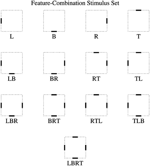
Figure 19. Merged feature objects. All members of the full object set are shown, using a dotted line to represent the central 32 × 32 square on which the individual features are positioned, with the features themselves shown as dark line segments. Nomenclature is by acronym of the features present, where T, top; B, bottom; L, left; and R, right. (After Elliffe et al., 2002.)

To train the network a stimulus was presented in a randomized sequence of nine locations in a square grid across the 128 × 128 input retina of VisNet2. The central location of the square grid was in the center of the “retina,” and the eight other locations were offset 8 pixels horizontally and/or vertically from this. Two different learning rules were used, “Hebbian” (16), and “trace” (17), and also an untrained condition with random weights. As in earlier work (Wallis and Rolls, 1997; Rolls and Milward, 2000) only the trace rule led to any cells with invariant responses, and the results shown are for networks trained with the trace rule.

The results with VisNet trained on the set of stimuli shown in Figure 19 with the trace rule are as follows. First, it was found that single neurons in the top layer learned to differentiate between the stimuli in that the responses of individual neurons were maximal for one of the stimuli and had no response to any of the other stimuli invariantly with respect to location. Moreover, the translation invariance was perfect for every stimulus (by different neurons) over every location (for all stimuli except “RTL” and “TLBR”).

The results presented show clearly that the VisNet paradigm can accommodate networks that can perform invariant discrimination of objects that have a subset–superset relationship. The result has important consequences for feature binding and for discriminating stimuli for other stimuli which may be supersets of the first stimulus. For example, a VisNet cell which responds invariantly to feature combination TL can genuinely signal the presence of exactly that combination, and will not necessarily be activated by T alone, or by TLB. The basis for this separation by competitive networks of stimuli which are subsets and supersets of each other is described by Rolls and Treves, 1998, Section 4.3.6) and by Rolls (2008b).

5.4.5. Feature binding in a hierarchical network with invariant representations of local feature combinations

In this section we consider the ability of output layer neurons to learn new stimuli if the lower layers are trained solely through exposure to simpler feature combinations from which the new stimuli are composed. A key question we address is how invariant representations of low-order feature combinations in the early layers of the visual system are able to uniquely specify the correct spatial arrangement of features in the overall stimulus and contribute to preventing false recognition errors in the output layer.

The problem, and its proposed solution, can be treated as follows. Consider an object 1234 made from the features 1, 2, 3, and 4. The invariant low-order feature combinations might represent 12, 23, and 34. Then if neurons at the next layer respond to combinations of the activity of these neurons, the only neurons in the next layer that would respond would be those tuned to 1234, not to, for example, 3412, which is distinguished from 1234 by the input of a pair neuron responding to 41 rather than to 23. The argument (Rolls, 1992) is that low-order spatial-feature combination neurons in the early stage contain sufficient spatial information so that a particular combination of those low-order feature combination neurons specifies a unique object, even if the relative positions of the low-order feature combination neurons are not known, because they are somewhat invariant.

The architecture of VisNet is intended to solve this problem partly by allowing high-spatial precision combinations of input features to be formed in layer 1. The actual input features in VisNet are, as described above, the output of oriented spatial-frequency tuned filters, and the combinations of these formed in layer 1 might thus be thought of in a simple way as, for example, a T or an L or for that matter a Y. Then in layer 2, application of the trace rule might enable neurons to respond to a T with limited spatial invariance (limited to the size of the region of layer 1 from which layer 2 cells receive their input). Then an “object” such as H might be formed at a higher layer because of a conjunction of two Ts in the same small region.

To show that VisNet can actually solve this problem, Elliffe et al. (2002) performed the experiments described next. They trained the first two layers of VisNet with feature pair combinations, forming representations of feature pairs with some translation invariance in layer 2. Then they used feature triples as input stimuli, allowed no more learning in layers 1 and 2, and then investigated whether layers 3 and 4 could be trained to produce invariant representations of the triples where the triples could only be distinguished if the local spatial arrangement of the features within the triple had effectively to be encoded in order to distinguish the different triples. For this experiment, they needed stimuli that could be specified in terms of a set of different features (they chose vertical (1), diagonal (2), and horizontal (3) bars) each capable of being shown at a set of different relative spatial positions (designated A, B, and C), as shown in Figure 20.

FIGURE 20

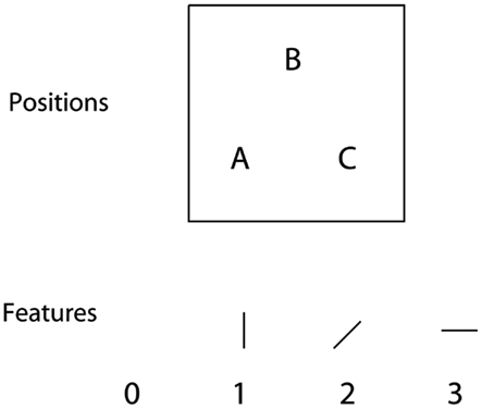
Figure 20. Feature combinations for experiments of Section 5.4.5: there are 3 features denoted by 1, 2, and 3 (including a blank space 0) that can be placed in any of 3 positions A, B, and C. Individual stimuli are denoted by three consecutive numbers which refer to the individual features present in positions A, B, and C, respectively. In the experiments in Section 5.4.5, layers 1 and 2 were trained on stimuli consisting of pairs of the features, and layers 3 and 4 were trained on stimuli consisting of triples. Then the network was tested to show whether layer 4 neurons would distinguish between triples, even though the first two layers had only been trained on pairs. In addition, the network was tested to show whether individual cells in layer 4 could distinguish between triples even in locations where the triples were not presented during training. (After Elliffe et al., 2002.)

The stimuli are thus defined in terms of what features are present and their precise spatial arrangement with respect to each other. The length of the horizontal and vertical feature bars shown in Figure 20 is 8 pixels. To train the network a stimulus (that is a pair or triple feature combination) is presented in a randomized sequence of nine locations in a square grid across the 128 × 128 input retina. The central location of the square grid is in the center of the “retina,” and the eight other locations are offset 8 pixels horizontally and/or vertically from this. We refer to the two and three feature stimuli as “pairs” and “triples,” respectively. Individual stimuli are denoted by three numbers which refer to the individual features present in positions A, B and C, respectively. For example, a stimulus with positions A and C containing a vertical and diagonal bar, respectively, would be referred to as stimulus 102, where the 0 denotes no feature present in position B. In total there are 18 pairs (120, 130, 210, 230, 310, 320, 012, 013, 021, 023, 031, 032, 102, 103, 201, 203, 301, 302) and 6 triples (123, 132, 213, 231, 312, 321). This nomenclature not only defines which features are present within objects, but also the spatial relationships of their component features. Then the computational problem can be illustrated by considering the triple 123. If invariant representations are formed of single features, then there would be no way that neurons higher in the hierarchy could distinguish the object 123 from 213 or any other arrangement of the three features. An approach to this problem (see, e.g., Rolls, 1992) is to form early on in the processing neurons that respond to overlapping combinations of features in the correct spatial arrangement, and then to develop invariant representations in the next layer from these neurons which already contain evidence on the local spatial arrangement of features. An example might be that with the object 123, the invariant feature pairs would represent 120, 023, and 103. Then if neurons at the next layer correspond to combinations of these neurons, the only next layer neurons that would respond would be those tuned to 123, not to, for example, 213. The argument is that the low-order spatial-feature combination neurons in the early stage contain sufficient spatial information so that a particular combination of those low-order feature combination neurons specifies a unique object, even if the relative positions of the low-order feature combination neurons are not known because these neurons are somewhat translation-invariant (cf. also Fukushima, 1988).

The stimuli used in the experiments of Elliffe et al. (2002) were constructed from pre-processed component features as discussed in Section 5.4.4. That is, base stimuli containing a single feature were constructed and filtered, and then the pairs and triples were constructed by merging these pre-processed single feature images. In the first experiment layers 1 and 2 of VisNet were trained with the 18 feature pairs, each stimulus being presented in sequences of 9 locations across the input. This led to the formation of neurons that responded to the feature pairs with some translation invariance in layer 2. Then they trained layers 3 and 4 on the 6 feature triples in the same 9 locations, while allowing no more learning in layers 1 and 2, and examined whether the output layer of VisNet had developed transform invariant neurons to the 6 triples. The idea was to test whether layers 3 and 4 could be trained to produce invariant representations of the triples where the triples could only be distinguished if the local spatial arrangement of the features within the triple had effectively to be encoded in order to distinguish the different triples. The results from this experiment were compared and contrasted with results from three other experiments which involved different training regimes for layers 1, 2 and layers 3, 4. All four experiments are summarized in Table 5. Experiment 2 involved no training in layers 1, 2 and 3, 4, with the synaptic weights left unchanged from their initial random values. These results are included as a baseline performance with which to compare results from the other experiments 1, 3, and 4. The model parameters used in these experiments were as described by Rolls and Milward (2000) and Rolls and Stringer (2001).

TABLE 5

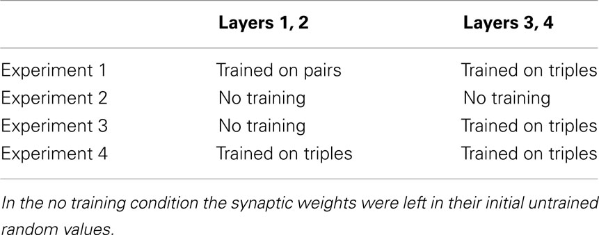
Table 5. The different training regimes used in VisNet experiments 1–4 of Section 5.4.5.

In Figure 21 we present numerical results for the four experiments listed in Table 5. On the left are the single cell information measures for all top (4th) layer neurons ranked in order of their invariance to the triples, while on the right are multiple cell information measures. To help to interpret these results we can compute the maximum single cell information measure according to

FIGURE 21

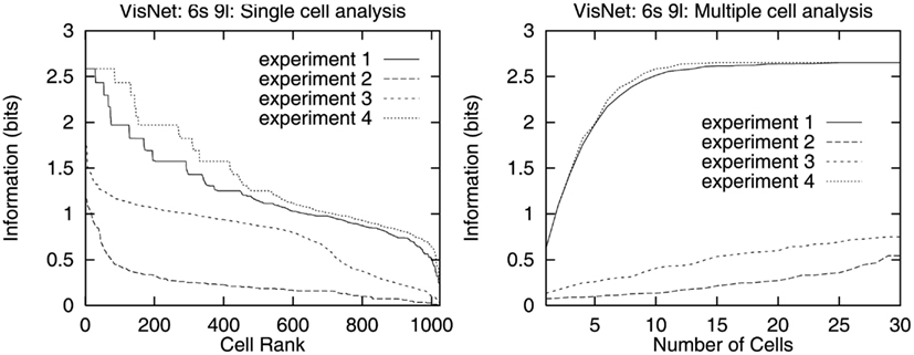
Figure 21. Numerical results for experiments 1–4 as described in Table 5, with the trace-learning rule (17). On the left are single cell information measures, and on the right are multiple cell information measures. (After Elliffe et al., 2002.)

$\text{Maximum single cell information}={log}_2\left(\text{Number of triples}\right),$ (42)

where the number of triples is 6. This gives a maximum single cell information measure of 2.6 bits for these test cases. First, comparing the results for experiment 1 with the baseline performance of experiment 2 (no training) demonstrates that even with the first two layers trained to form invariant responses to the pairs, and then only layers 3 and 4 trained on feature triples, layer 4 is indeed capable of developing translation-invariant neurons that can discriminate effectively between the 6 different feature triples. Indeed, from the single cell information measures it can be seen that a number of cells have reached the maximum level of performance in experiment 1. In addition, the multiple cell information analysis presented in Figure 21 shows that all the stimuli could be discriminated from each other by the firing of a number of cells. Analysis of the response profiles of individual cells showed that a fourth layer cell could respond to one of the triple feature stimuli and have no response to any other of the triple feature stimuli invariantly with respect to location.

A comparison of the results from experiment 1 with those from experiment 3 (see Table 5 and Figure 21) reveals that training the first two layers to develop neurons that respond invariantly to the pairs (performed in experiment 1) actually leads to improved invariance of 4th layer neurons to the triples, as compared with when the first two layers are left untrained (experiment 3).

Two conclusions follow from these results (Elliffe et al., 2002). First, a hierarchical network that seeks to produce invariant representations in the way used by VisNet can solve the feature binding problem. In particular, when feature pairs in layer 2 with some translation invariance are used as the input to later layers, these later layers can nevertheless build invariant representations of objects where all the individual features in the stimulus must occur in the correct spatial position relative to each other. This is possible because the feature combination neurons formed in the first layer (which could be trained just with a Hebb rule) do respond to combinations of input features in the correct spatial configuration, partly because of the limited size of their receptive fields. The second conclusion is that even though early layers can in this case only respond to small feature subsets, these provide, with no further training of layers 1 and 2, an adequate basis for learning to discriminate in layers 3 and 4 stimuli consisting of combinations of larger numbers of features. Indeed, comparing results from experiment 1 with experiment 4 (in which all layers were trained on triples, see Table 5) demonstrates that training the lower layer neurons to develop invariant responses to the pairs offers almost as good performance as training all layers on the triples (see Figure 21).

5.4.6. Stimulus generalization to untrained transforms of new objects

Another important aspect of the architecture of VisNet is that it need not be trained with every stimulus in every possible location. Indeed, part of the hypothesis (Rolls, 1992) is that training early layers (e.g., 1–3) with a wide range of visual stimuli will set up feature analyzers in these early layers which are appropriate later on with no further training of early layers for new objects. For example, presentation of a new object might result in large numbers of low-order feature combination neurons in early layers of VisNet being active, but the particular set of feature combination neurons active would be different for the new object. The later layers of the network (in VisNet, layer 4) would then learn this new set of active layer 3 neurons as encoding the new object. However, if the new object was then shown in a new location, the same set of layer 3 neurons would be active because they respond with spatial invariance to feature combinations, and given that the layer 3–4 connections had already been set up by the new object, the correct layer 4 neurons would be activated by the new object in its new untrained location, and without any further training.

To test this hypothesis Elliffe et al. (2002) repeated the general procedure of experiment 1 of Section 5.4.5, training layers 1 and 2 with feature pairs, but then instead trained layers 3 and 4 on the triples in only 7 of the original 9 locations. The crucial test was to determine whether VisNet could form top layer neurons that responded invariantly to the 6 triples when presented over all nine locations, not just the seven locations at which the triples had been presented during training.

It was found that VisNet is still able to develop some fourth layer neurons with perfect invariance, that is which have invariant responses over all nine locations, as shown by the single cell information analysis. The response profiles of individual fourth layer cells showed that they can continue to discriminate between the triples even in the two locations where the triples were not presented during training. In addition, the multiple cell analysis showed that a small population of cells was able to discriminate between all of the stimuli irrespective of location, even though for two of the test locations the triples had not been trained at those particular locations during the training of layers 3 and 4.

The use of transformation rules learned by early stages of the hierarchy to enable later stages to perform correctly on transformed views never seen before of objects is now being investigated by others (Leibo et al., 2010).

5.4.7. Discussion of feature binding in hierarchical layered networks

Elliffe et al. (2002) thus first showed (see Section 5.4.4) that hierarchical feature-detecting neural networks can learn to respond differently to stimuli that consist of unique combinations of non-unique input features, and that this extends to stimuli that are direct subsets or supersets of the features present in other stimuli.

Second Elliffe et al. (2002) investigated (see Section 5.4.5) the hypothesis that hierarchical layered networks can produce identification of unique stimuli even when the feature combination neurons used to define the stimuli are themselves partly translation-invariant. The stimulus identification should work correctly because feature combination neurons in which the spatial features are bound together with high-spatial precision are formed in the first layer. Then at later layers when neurons with some translation invariance are formed, the neurons nevertheless contain information about the relative spatial position of the original features. There is only then one object which will be consistent with the set of active neurons at earlier layers, which though somewhat translation-invariant as combination neurons, reflect in the activity of each neuron information about the original spatial position of the features. I note that the trace rule training used in early layers (1 and 2) in Experiments 1 and 4 would set up partly invariant feature combination neurons, and yet the late layers (3 and 4) were able to produce during training neurons in layer 4 that responded to stimuli that consisted of unique spatial arrangements of lower order feature combinations. Moreover, and very interestingly Elliffe et al. (2002) were able to demonstrate that VisNet layer 4 neurons would respond correctly to visual stimuli at untrained locations, provided that the feature subsets had been trained in early layers of the network at all locations, and that the whole stimulus had been trained at some locations in the later layers of the network.

The results described by Elliffe et al. (2002) thus provide one solution to the feature binding problem. The solution which has been shown to work in the model is that in a multilayer competitive network, feature combination neurons which encode the spatial arrangement of the bound features are formed at intermediate layers of the network. Then neurons at later layers of the network which respond to combinations of active intermediate-layer neurons do contain sufficient evidence about the local spatial arrangement of the features to identify stimuli because the local spatial arrangement is encoded by the intermediate-layer neurons. The information required to solve the visual feature binding problem thus becomes encoded by self-organization into what become hard-wired properties of the network. In this sense, feature binding is not solved at run-time by the necessity to instantaneously set up arbitrary syntactic links between sets of co-active neurons. The computational solution proposed to the superset/subset aspect of the binding problem will apply in principle to other multilayer competitive networks, although the issues considered here have not been explicitly addressed in architectures such as the Neocognitron (Fukushima and Miyake, 1982).

Consistent with these hypotheses about how VisNet operates to achieve, by layer 4, position-invariant responses to stimuli defined by combinations of features in the correct spatial arrangement, investigations of the effective stimuli for neurons in intermediate layers of VisNet showed as follows. In layer 1, cells responded to the presence of individual features, or to low-order combinations of features (e.g., a pair of features) in the correct spatial arrangement at a small number of nearby locations. In layers 2 and 3, neurons responded to single features or to higher order combinations of features (e.g., stimuli composed of feature triples) in more locations. These findings provide direct evidence that VisNet does operate as described above to solve the feature binding problem.

A further issue with hierarchical multilayer architectures such as VisNet is that false binding errors might occur in the following way (Mozer, 1991; Mel and Fiser, 2000). Consider the output of one-layer in such a network in which there is information only about which pairs are present. How then could a neuron in the next layer discriminate between the whole stimulus (such as the triple 123 in the above experiment) and what could be considered a more distributed stimulus or multiple different stimuli composed of the separated subparts of that stimulus (e.g., the pairs 120, 023, 103 occurring in 3 of the 9 training locations in the above experiment)? The problem here is to distinguish a single object from multiple other objects containing the same component combinations (e.g., pairs). We propose that part of the solution to this general problem in real visual systems is implemented through lateral inhibition between neurons in individual layers, and that this mechanism, implemented in VisNet, acts to reduce the possibility of false recognition errors in the following two ways.

First, consider the situation in which neurons in layer N have learned to represent low-order feature combinations with location invariance, and where a neuron n in layer N + 1 has learned to respond to a particular set Ω of these feature combinations. The problem is that neuron n receives the same input from layer N as long as the same set Ω of feature combinations is present, and cannot distinguish between different spatial arrangements of these feature combinations. The question is how can neuron n respond only to a particular favored spatial arrangement Ψ of the feature combinations contained within the set Ω. We suggest that as the favored spatial arrangement Ψ is altered by rearranging the spatial relationships of the component feature combinations, the new feature combinations that are formed in new locations will stimulate additional neurons nearby in layer N + 1, and these will tend to inhibit the firing of neuron n. Thus, lateral inhibition within a layer will have the effect of making neurons more selective, ensuring neuron n responds only to a single spatial arrangement Ψ from the set of feature combinations Ω, and hence reducing the possibility of false recognition.

The second way in which lateral inhibition may help to reduce binding errors is through limiting the sparseness of neuronal firing rates within layers. In our discussion above the spurious stimuli we suggested that might lead to false recognition of triples were obtained from splitting up the component feature combinations (pairs) so that they occurred in separate training locations. However, this would lead to an increase in the number of features present in the complete stimulus; triples contain 3 features while their spurious counterparts would contain 6 features (resulting from 3 separate pairs). For this trivial example, the increase in the number of features is not dramatic, but if we consider, say, stimuli composed of 4 features where the component feature combinations represented by lower layers might be triples, then to form spurious stimuli we need to use 12 features (resulting from 4 triples occurring in separate locations). But if the lower layers also represented all possible pairs then the number of features required in the spurious stimuli would increase further. In fact, as the size of the stimulus increases in terms of the number of features, and as the size of the component feature combinations represented by the lower layers increases, there is a combinatorial explosion in terms of the number of features required as we attempt to construct spurious stimuli to trigger false recognition. And the construction of such spurious stimuli will then be prevented through setting a limit on the sparseness of firing rates within layers, which will in turn set a limit on the number of features that can be represented. Lateral inhibition is likely to contribute in both these ways to the performance of VisNet when the stimuli consist of subsets and supersets of each other, as described in Section 5.4.4.

Another way is which the problem of multiple objects is addressed is by limiting the size of the receptive fields of inferior temporal cortex neurons so that neurons in IT respond primarily to the object being fixated, but with nevertheless some asymmetry in the receptive fields (see Section 5.9). Multiple objects are then “seen” by virtue of being added to a visuo-spatial scratchpad (Rolls, 2008b).

A related issue that arises in this class of network is whether forming neurons that respond to feature combinations in the way described here leads to a combinatorial explosion in the number of neurons required. The solution to this issue that is proposed is to form only low-order combinations of features at any one stage of the network (Rolls, 1992; cf. Feldman, 1985). Using low-order combinations limits the number of neurons required, yet enables the type of computation that relies on feature combination neurons that is analyzed here to still be performed. The actual number of neurons required depends also on the redundancies present in the statistics of real-world images. Even given these factors, it is likely that a large number of neurons would be required if the ventral visual system performs the computation of invariant representations in the manner captured by the hypotheses implemented in VisNet. Consistent with this, a considerable part of the non-human primate brain is devoted to visual information processing. The fact that large numbers of neurons and a multilayer organization are present in the primate ventral visual system is actually thus consistent with the type of model of visual information processing described here.

5.5. Operation in a Cluttered Environment

In this section we consider how hierarchical layered networks of the type exemplified by VisNet operate in cluttered environments. Although there has been much work involving object recognition in cluttered environments with artificial vision systems, many such systems typically rely on some form of explicit segmentation followed by search and template matching procedure (see Ullman, 1996 for a general review). In natural environments, objects may not only appear against cluttered (natural) backgrounds, but also the object may be partially occluded. Biological nervous systems operate in quite a different manner to those artificial vision systems that rely on search and template matching, and the way in which biological systems cope with cluttered environments and partial occlusion is likely to be quite different also.

One of the factors that will influence the performance of the type of architecture considered here, hierarchically organized series of competitive networks, which form one class of approaches to biologically relevant networks for invariant object recognition (Fukushima, 1980; Poggio and Edelman, 1990; Rolls, 1992, 2008b; Wallis and Rolls, 1997; Rolls and Treves, 1998), is how lateral inhibition and competition are managed within a layer. Even if an object is not obscured, the effect of a cluttered background will be to fire additional neurons, which will in turn to some extent compete with and inhibit those neurons that are specifically tuned to respond to the desired object. Moreover, where the clutter is adjacent to part of the object, the feature analyzing neurons activated against a blank background might be different from those activated against a cluttered background, if there is no explicit segmentation process. We consider these issues next, following investigations of Stringer and Rolls (2000).

5.5.1. VisNet simulations with stimuli in cluttered backgrounds

In this section we show that recognition of objects learned previously against a blank background is hardly affected by the presence of a natural cluttered background. We go on to consider what happens when VisNet is set the task of learning new stimuli presented against cluttered backgrounds.

The images used for training and testing VisNet in the simulations described next performed by Stringer and Rolls (2000) were specially constructed. There were 7 face stimuli approximately 64 pixels in height constructed without backgrounds. In addition there were 3 possible backgrounds: a blank background (gray-scale 127, where the range is 0–255), and two cluttered backgrounds as shown in Figure 22 which are 128 × 128 pixels in size. Each image presented to VisNet’s 128 × 128 input retina was composed of a single face stimulus positioned at one of 9 locations on either a blank or cluttered background. The cluttered background was intended to be like the background against which an object might be viewed in a natural scene. If a background is used in an experiment described here, the same background is always used, and it is always in the same position, with stimuli moved to different positions on it. The 9 stimulus locations are arranged in a square grid across the background, where the grid spacings are 32 pixels horizontally or vertically. Before images were presented to VisNet’s input layer they were pre-processed by the standard set of input filters which accord with the general tuning profiles of simple cells in V1 (Hawken and Parker, 1987); full details are given in Rolls and Milward (2000). To train the network a sequence of images is presented to VisNet’s retina that corresponds to a single stimulus occurring in a randomized sequence of the 9 locations across a background. At each presentation the activation of individual neurons is calculated, then their firing rates are calculated, and then the synaptic weights are updated. After a stimulus has been presented in all the training locations, a new stimulus is chosen at random and the process repeated. The presentation of all the stimuli across all locations constitutes 1 epoch of training. In this manner the network is trained one-layer at a time starting with layer 1 and finishing with layer 4. In the investigations described in this subsection, the numbers of training epochs for layers 1–4 were 50, 100, 100, and 75, respectively.

FIGURE 22

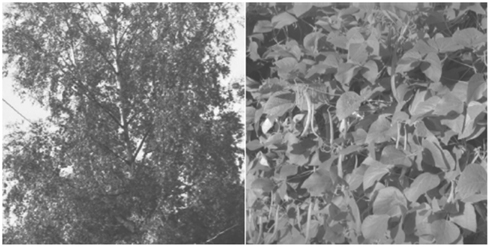
Figure 22. Cluttered backgrounds used in VisNet simulations: backgrounds 1 and 2 are on the left and right, respectively.

In this experiment (see Stringer and Rolls, 2000, experiment 2), VisNet was trained with the 7 face stimuli presented on a blank background, but tested with the faces presented on each of the 2 cluttered backgrounds.

The single and multiple cell information showed perfect performance. Compared to performance when shown against a blank background, there was very little deterioration in performance when testing with the faces presented on either of the two cluttered backgrounds.

This is an interesting result to compare with many artificial vision systems that would need to carry out computationally intensive serial searching and template matching procedures in order to achieve such results. In contrast, the VisNet neural network architecture is able to perform such recognition relatively quickly through a simple feed-forward computation.

Further results from this experiment showed that different neurons can achieve excellent invariant responses to each of the 7 faces even with the faces presented on a cluttered background. The response profiles are independent of location but differentiate between the faces in that the responses are maximal for only one of the faces and minimal for all other faces.

This is an interesting and important result, for it shows that after learning, special mechanisms for segmentation and for attention are not needed in order for neurons already tuned by previous learning to the stimuli to be activated correctly in the output layer. Although the experiments described here tested for position invariance, we predict and would expect that the same results would be demonstrable for size and view-invariant representations of objects.

In experiments 3 and 4 of Stringer and Rolls (2000), VisNet was trained with the 7 face stimuli presented on either one of the 2 cluttered backgrounds, but tested with the faces presented on a blank background. Results for this experiment showed poor performance. The results of experiments 3 and 4 suggest that in order for a cell to learn invariant responses to different transforms of a stimulus when it is presented during training in a cluttered background, some form of segmentation is required in order to separate the Figure (i.e., the stimulus or object) from the background. This segmentation might be performed using evidence in the visual scene about different depths, motions, colors, etc. of the object from its background. In the visual system, this might mean combining evidence represented in different cortical areas, and might be performed by cross-connections between cortical areas to enable such evidence to help separate the representations of objects from their backgrounds in the form-representing cortical areas.

Another mechanism that helps the operation of architectures such as VisNet and the primate visual system to learn about new objects in cluttered scenes is that the receptive fields of inferior temporal cortex neurons become much smaller when objects are seen against natural backgrounds (Sections 5.8.1 and 5.8). This will help greatly to learn about new objects that are being fixated, by reducing responsiveness to other features elsewhere in the scene.

Another mechanism that might help the learning of new objects in a natural scene is attention. An attentional mechanism might highlight the current stimulus being attended to and suppress the effects of background noise, providing a training representation of the object more like that which would be produced when it is presented against a blank background. The mechanisms that could implement such attentional processes are described elsewhere (Rolls, 2008b). If such attentional mechanisms do contribute to the development of view-invariance, then it follows that cells in the temporal cortex may only develop transform invariant responses to objects to which attention is directed.

Part of the reason for the poor performance in experiments 3 and 4 was probably that the stimuli were always presented against the same fixed background (for technical reasons), and thus the neurons learned about the background rather than the stimuli. Part of the difficulty that hierarchical multilayer competitive networks have with learning in cluttered environments may more generally be that without explicit segmentation of the stimulus from its background, at least some of the features that should be formed to encode the stimuli are not formed properly, because the neurons learn to respond to combinations of inputs which come partly from the stimulus, and partly from the background. To investigate this Stringer and Rolls (2000) performed experiment 5 in which layers 1–3 were pre-trained with stimuli to ensure that good feature combination neurons for stimuli were available, and then allowed learning in only layer 4 when stimuli were presented in the cluttered backgrounds. Layer 4 was then trained in the usual way with the 7 faces presented against a cluttered background. The results showed that prior random exposure to the face stimuli led to much improved performance.

These results demonstrated that the problem of developing position-invariant neurons to stimuli occurring against cluttered backgrounds may be ameliorated by the prior existence of stimulus-tuned feature-detecting neurons in the early layers of the visual system, and that these feature-detecting neurons may be set up through previous exposure to the relevant class of objects. When tested in cluttered environments, the background clutter may of course activate some other neurons in the output layer, but at least the neurons that have learned to respond to the trained stimuli are activated. The result of this activity is sufficient for the activity in the output layer to be useful, in the sense that it can be read-off correctly by a pattern associator connected to the output layer. Indeed, Stringer and Rolls (2000) tested this by connecting a pattern associator to layer 4 of VisNet. The pattern associator had seven neurons, one for each face, and 1,024 inputs, one from each neuron in layer 4 of VisNet. The pattern associator learned when trained with a simple associative Hebb rule (equation (16)) to activate the correct output neuron whenever one of the faces was shown in any position in the uncluttered environment. This ability was shown to be dependent on invariant neurons for each stimulus in the output layer of VisNet, for the pattern associator could not be taught the task if VisNet had not been previously trained with a trace-learning rule to produce invariant representations. Then it was shown that exactly the correct neuron was activated when any of the faces was shown in any position with the cluttered background. This read-off by a pattern associator is exactly what we hypothesize takes place in the brain, in that the inferior temporal visual cortex (where neurons with invariant responses are found) projects to structures such as the orbitofrontal cortex and amygdala, where associations between the invariant visual representations and stimuli such as taste and touch are learned (Rolls and Treves, 1998; Rolls, 1999, 2005, 2008b, 2013; Rolls and Grabenhorst, 2008; Grabenhorst and Rolls, 2011). Thus testing whether the output of an architecture such as VisNet can be used effectively by a pattern associator is a very biologically relevant way to evaluate the performance of this class of architecture.

5.5.2. Learning invariant representations of an object with multiple objects in the scene and with cluttered backgrounds

The results of the experiments just described suggest that in order for a neuron to learn invariant responses to different transforms of a stimulus when it is presented during training in a cluttered background, some form of segmentation is required in order to separate the figure (i.e., the stimulus or object) from the background. This segmentation might be performed using evidence in the visual scene about different depths, motions, colors, etc. of the object from its background. In the visual system, this might mean combining evidence represented in different cortical areas, and might be performed by cross-connections between cortical areas to enable such evidence to help separate the representations of objects from their backgrounds in the form-representing cortical areas.

A second way in which training a feature hierarchy network in a cluttered natural scene may be facilitated follows from the finding that the receptive fields of inferior temporal cortex neurons shrink from in the order of 70° in diameter when only one object is present in a blank scene to much smaller values of as little as 5–10° close to the fovea in complex natural scenes (Rolls et al., 2003). The proposed mechanism for this is that if there is an object at the fovea, this object, because of the high-cortical magnification factor at the fovea, dominates the activity of neurons in the inferior temporal cortex by competitive interactions (Trappenberg et al., 2002; Deco and Rolls, 2004; see Section 5.8). This allows primarily the object at the fovea to be represented in the inferior temporal cortex, and, it is proposed, for learning to be about this object, and not about the other objects in a whole scene.

Third, top-down spatial attention (Deco and Rolls, 2004, 2005a; Rolls, 2008b) could bias the competition toward a region of visual space where the object to be learned is located.

Fourth, if object 1 is presented during training with other different objects present on different trials, then the competitive networks that are part of VisNet will learn to represent each object separately, because the features that are part of each object will be much more strongly associated together, than are those features with the other features present in the different objects seen on some trials during training (Stringer et al., 2007; Stringer and Rolls, 2008). It is a natural property of competitive networks that input features that co-occur very frequently together are allocated output neurons to represent the pattern as a result of the learning. Input features that do not co-occur frequently, may not have output neurons allocated to them. This principle may help feature hierarchy systems to learn representations of individual objects, even when other objects with some of the same features are present in the visual scene, but with different other objects on different trials. With this fundamental and interesting property of competitive networks, it has now become possible for VisNet to self-organize invariant representations of individual objects, even though each object is always presented during training with at least one other object present in the scene (Stringer et al., 2007; Stringer and Rolls, 2008). This has been extended to learning separate representations of face expression and face identity from the same set of images, depending on the statistics with which the images are presented (Tromans et al., 2011); and learning separate representations of independently rotating objects (Tromans et al., 2012).

5.5.3. VisNet simulations with partially occluded stimuli

In this section we examine the recognition of partially occluded stimuli. Many artificial vision systems that perform object recognition typically search for specific markers in stimuli, and hence their performance may become fragile if key parts of a stimulus are occluded. However, in contrast we demonstrate that the model of invariance learning in the brain discussed here can continue to offer robust performance with this kind of problem, and that the model is able to correctly identify stimuli with considerable flexibility about what part of a stimulus is visible.

In these simulations (Stringer and Rolls, 2000), training and testing was performed with a blank background to avoid confounding the two separate problems of occlusion and background clutter. In object recognition tasks, artificial vision systems may typically rely on being able to locate a small number of key markers on a stimulus in order to be able to identify it. This approach can become fragile when a number of these markers become obscured. In contrast, biological vision systems may generalize or complete from a partial input as a result of the use of distributed representations in neural networks, and this could lead to greater robustness in situations of partial occlusion.

In this experiment (6 of Stringer and Rolls, 2000), the network was first trained with the 7 face stimuli without occlusion, but during testing there were two options: either (i) the top halves of all the faces were occluded or (ii) the bottom halves of all the faces were occluded. Since VisNet was tested with either the top or bottom half of the stimuli no stimulus features were common to the two test options. This ensures that if performance is good with both options, the performance cannot be based on the use of a single feature to identify a stimulus. Results for this experiment are shown in Figure 23, with single and multiple cell information measures on the left and right, respectively. When compared with the performance without occlusion (Stringer and Rolls, 2000), Figure 23 shows that there is only a modest drop in performance in the single cell information measures when the stimuli are partially occluded.

FIGURE 23

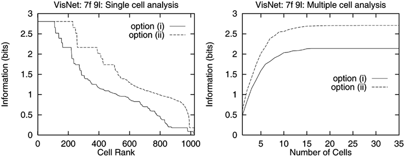
Figure 23. Effects of partial occlusion of a stimulus: numerical results for experiment 6 of Stringer and Rolls (2000), with the 7 faces presented on a blank background during both training and testing. Training was performed with the whole face. However, during testing there are two options: either (i) the top half of all the faces are occluded, or (ii) the bottom half of all the faces are occluded. On the left are single cell information measures, and on the right are multiple cell information measures.

For both options (i) and (ii), even with partially occluded stimuli, a number of cells continue to respond maximally to one preferred stimulus in all locations, while responding minimally to all other stimuli. However, comparing results from options (i) and (ii) shows that the network performance is better when the bottom half of the faces is occluded. This is consistent with psychological results showing that face recognition is performed more easily when the top halves of faces are visible rather than the bottom halves (see Bruce, 1988). The top half of a face will generally contain salient features, e.g., eyes and hair, that are particularly helpful for recognition of the individual, and it is interesting that these simulations appear to further demonstrate this point. Furthermore, the multiple cell information measures confirm that performance is better with the upper half of the face visible (option (ii)) than the lower half (option (i)). When the top halves of the faces are occluded the multiple cell information measure asymptotes to a suboptimal value reflecting the difficulty of discriminating between these more difficult images.

Thus this model of the ventral visual system offers robust performance with this kind of problem, and the model is able to correctly identify stimuli with considerable flexibility about what part of a stimulus is visible, because it is effectively using distributed representations and associative processing.

5.6. Learning 3D Transforms

In this section we describe investigations of Stringer and Rolls (2002) which show that trace-learning can in the VisNet architecture solve the problem of in-depth rotation invariant object recognition by developing representations of the transforms which features undergo when they are on the surfaces of 3D objects. Moreover, it is shown that having learned how features on 3D objects transform as the object is rotated in-depth, the network can correctly recognize novel 3D variations within a generic view of an object which is composed of previously learned feature combinations.

Rolls’ hypothesis of how object recognition could be implemented in the brain postulates that trace rule learning helps invariant representations to form in two ways (Rolls, 1992, 1994, 1995, 2000). The first process enables associations to be learned between different generic 3D views of an object where there are different qualitative shape descriptors. One example of this would be the front and back views of an object, which might have very different shape descriptors. Another example is provided by considering how the shape descriptors typical of 3D shapes, such as Y vertices, arrow vertices, cusps, and ellipse shapes, alter when most 3D objects are rotated in 3 dimensions. At some point in the 3D rotation, there is a catastrophic rearrangement of the shape descriptors as a new generic view can be seen (Koenderink, 1990). An example of a catastrophic change to a new generic view is when a cup being viewed from slightly below is rotated so that one can see inside the cup from slightly above. The bottom surface disappears, the top surface of the cup changes from a cusp to an ellipse, and the inside of the cup with a whole set of new features comes into view. The second process is that within a generic view, as the object is rotated in-depth, there will be no catastrophic changes in the qualitative 3D shape descriptors, but instead the quantitative values of the shape descriptors alter. For example, while the cup is being rotated within a generic view seen from somewhat below, the curvature of the cusp forming the top boundary will alter, but the qualitative shape descriptor will remain a cusp. Trace-learning could help with both processes. That is, trace-learning could help to associate together qualitatively different sets of shape descriptors that occur close together in time, and describe, for example, the generically different views of a cup. Trace-learning could also help with the second process, and learn to associate together the different quantitative values of shape descriptors that typically occur when objects are rotated within a generic view.

We note that there is evidence that some neurons in the inferior temporal cortex may show the two types of 3D invariance. First Booth and Rolls (1998) showed that some inferior temporal cortex neurons can respond to different generic views of familiar 3D objects. Second, some neurons do generalize across quantitative changes in the values of 3D shape descriptors while faces (Hasselmo et al., 1989b) and objects (Logothetis et al., 1995; Tanaka, 1996) are rotated within-generic views. Indeed, Logothetis et al. (1995) showed that a few inferior temporal cortex neurons can generalize to novel (untrained) values of the quantitative shape descriptors typical of within-generic view object rotation.

In addition to the qualitative shape descriptor changes that occur catastrophically between different generic views of an object, and the quantitative changes of 3D shape descriptors that occur within a generic view, there is a third type of transform that must be learned for correct invariant recognition of 3D objects as they rotate in-depth. This third type of transform is that which occurs to the surface features on a 3D object as it transforms in-depth. The main aim here is to consider mechanisms that could enable neurons to learn this third type of transform, that is how to generalize correctly over the changes in the surface markings on 3D objects that are typically encountered as 3D objects rotate within a generic view. Examples of the types of perspectival transforms investigated are shown in Figure 24. Surface markings on the sphere that consist of combinations of three features in different spatial arrangements undergo characteristic transforms as the sphere is rotated from 0° to −60° and +60°. We investigated whether the class of architecture exemplified by VisNet, and the trace-learning rule, can learn about the transforms that surface features of 3D objects typically undergo during 3D rotation in such a way that the network generalizes across the change of the quantitative values of the surface features produced by the rotation, and yet still discriminates between the different objects (in this case spheres). In the cases being considered, each object is identified by surface markings that consist of a different spatial arrangement of the same three features (a horizontal, vertical, and diagonal line, which become arcs on the surface of the object).

FIGURE 24

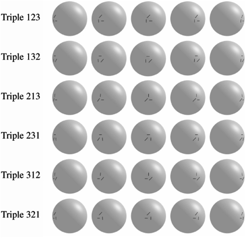
Figure 24. Learning 3D perspectival transforms of features. Representations of the 6 visual stimuli with 3 surface features (triples) presented to VisNet during the simulations described in Section 5.6. Each stimulus is a sphere that is uniquely identified by a unique combination of three surface features (a vertical, diagonal, and horizontal arc), which occur in 3 relative positions A, B, and C. Each row shows one of the stimuli rotated through the 5 different rotational views in which the stimulus is presented to VisNet. From left to right the rotational views shown are: (i) –60°, (ii) –30°, (iii) 0° (central position), (iv) +30°, and (v) +60°. (After Stringer and Rolls, 2002.)

We note that it has been suggested that the finding that neurons may offer some degree of 3D rotation invariance after training with a single view (or limited set of views) represents a challenge for existing trace-learning models, because these models assume that an initial exposure is required during learning to every transformation of the object to be recognized (Riesenhuber and Poggio, 1998). Stringer and Rolls (2002) showed as described here that this is not the case, and that such models can generalize to novel within-generic views of an object provided that the characteristic changes that the features show as objects are rotated have been learned previously for the sets of features when they are present in different objects.

Elliffe et al. (2002) demonstrated for a 2D system how the existence of translation-invariant representations of low-order feature combinations in the early layers of the visual system could allow correct stimulus identification in the output layer even when the stimulus was presented in a novel location where the stimulus had not previously occurred during learning. The proposal was that the low-order spatial-feature combination neurons in the early stages contain sufficient spatial information so that a particular combination of those low-order feature combination neurons specifies a unique object, even if the relative positions of the low-order feature combination neurons are not known because these neurons are somewhat translation-invariant (see Section 5.4.5). Stringer and Rolls (2002) extended this analysis to feature combinations on 3D objects, and indeed in their simulations described in this section therefore used surface markings for the 3D objects that consisted of triples of features.

The images used for training and testing VisNet were specially constructed for the purpose of demonstrating how the trace-learning paradigm might be further developed to give rise to neurons that are able to respond invariantly to novel within-generic view perspectives of an object, obtained by rotations in-depth up to 30° from any perspectives encountered during learning. The stimuli take the form of the surface feature combinations of 3-dimensional rotating spheres, with each image presented to VisNet’s retina being a 2-dimensional projection of the surface features of one of the spheres. Each stimulus is uniquely identified by two or three surface features, where the surface features are (1) vertical, (2) diagonal, and (3) horizontal arcs, and where each feature may be centered at three different spatial positions, designated A, B, and C, as shown in Figure 24. The stimuli are thus defined in terms of what features are present and their precise spatial arrangement with respect to each other. We refer to the two and three feature stimuli as “pairs” and “triples,” respectively. Individual stimuli are denoted by three numbers which refer to the individual features present in positions A, B and C, respectively. For example, a stimulus with positions A and C containing a vertical and diagonal bar, respectively, would be referred to as stimulus 102, where the 0 denotes no feature present in position B. In total there are 18 pairs (120, 130, 210, 230, 310, 320, 012, 013, 021, 023, 031, 032, 102, 103, 201, 203, 301, 302) and 6 triples (123, 132, 213, 231, 312, 321).

To train the network each stimulus was presented to VisNet in a randomized sequence of five orientations with respect to VisNet’s input retina, where the different orientations are obtained from successive in-depth rotations of the stimulus through 30°. That is, each stimulus was presented to VisNet’s retina from the following rotational views: (i) −60°, (ii) −30°, (iii) 0° (central position with surface features facing directly toward VisNet’s retina), (iv) 30°, and (v) 60°. Figure 24 shows representations of the 6 visual stimuli with 3 surface features (triples) presented to VisNet during the simulations. (For the actual simulations described here, the surface features and their deformations were what VisNet was trained and tested with, and the remaining blank surface of each sphere was set to the same gray-scale as the background.) Each row shows one of the stimuli rotated through the 5 different rotational views in which the stimulus is presented to VisNet. At each presentation the activation of individual neurons is calculated, then the neuronal firing rates are calculated, and then the synaptic weights are updated. Each time a stimulus has been presented in all the training orientations, a new stimulus is chosen at random and the process repeated. The presentation of all the stimuli through all 5 orientations constitutes 1 epoch of training. In this manner the network was trained one-layer at a time starting with layer 1 and finishing with layer 4. In the investigations described here, the numbers of training epochs for layers 1–4 were 50, 100, 100, and 75, respectively.

In experiment 1, VisNet was trained in two stages. In the first stage, the 18 feature pairs were used as input stimuli, with each stimulus being presented to VisNet’s retina in sequences of five orientations as described above. However, during this stage, learning was only allowed to take place in layers 1 and 2. This led to the formation of neurons which responded to the feature pairs with some rotation invariance in layer 2. In the second stage, we used the 6 feature triples as stimuli, with learning only allowed in layers 3 and 4. However, during this second training stage, the triples were only presented to VisNet’s input retina in the first 4 orientations (i–iv). After the two stages of training were completed Stringer and Rolls (2002) examined whether the output layer of VisNet had formed top layer neurons that responded invariantly to the 6 triples when presented in all 5 orientations, not just the 4 in which the triples had been presented during training. To provide baseline results for comparison, the results from experiment 1 were compared with results from experiment 2 which involved no training in layers 1, 2 and 3, 4, with the synaptic weights left unchanged from their initial random values.

In Figure 25 numerical results are given for the experiments described. On the left are the single cell information measures for all top (4th) layer neurons ranked in order of their invariance to the triples, while on the right are multiple cell information measures. To help to interpret these results we can compute the maximum single cell information measure according to

FIGURE 25

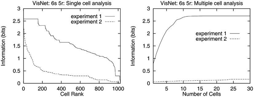
Figure 25. Learning 3D perspectival transforms of features. Numerical results for experiments 1 and 2: on the left are single cell information measures, and on the right are multiple cell information measures. (After Stringer and Rolls, 2002.)

$\text{Maximum\hspace{0.17em}single\hspace{0.17em}cell\hspace{0.17em}information\hspace{0.17em}}={\log }_2\left(\text{Number\hspace{0.17em}of\hspace{0.17em}triples}\right),$ (43)

where the number of triples is 6. This gives a maximum single cell information measure of 2.6 bits for these test cases. The information results from the experiment demonstrate that even with the triples presented to the network in only four of the five orientations during training, layer 4 is indeed capable of developing rotation invariant neurons that can discriminate effectively between the 6 different feature triples in all 5 orientations, that is with correct recognition from all five perspectives. In addition, the multiple cell information for the experiment reaches the maximal level of 2.6 bits, indicating that the network as a whole is capable of perfect discrimination between the 6 triples in any of the 5 orientations.

These results may be compared with the very poor baseline performance from the control experiment, where no learning was allowed before testing.

Stringer and Rolls (2002) also performed a control experiment to show that the network really had learned invariant representations specific to the kinds of 3D deformations undergone by the surface features as the objects rotated in-depth. In the control experiment the network was trained on “spheres” with non-deformed surface features; and then as predicted the network failed to operate correctly when it was tested with objects with the features present in the transformed way that they appear on the surface of a real 3D object.

Stringer and Rolls (2002) were thus able to show how trace-learning can form neurons that can respond invariantly to novel rotational within-generic view perspectives of an object, obtained by within-generic view 3D rotations up to 30° from any view encountered during learning. They were able to show in addition that this could occur for a novel view of an object which was not an interpolation from previously shown views. This was possible given that the low-order feature combination sets from which an object was composed had been learned about in early layers of VisNet previously. The within-generic view transform invariant object recognition described was achieved through the development of true 3-dimensional representations of objects based on 3-dimensional features and feature combinations, which, unlike 2-dimensional feature combinations, are invariant under moderate in-depth rotations of the object. Thus, in a sense, these rotation invariant representations encode a form of 3-dimensional knowledge with which to interpret the visual input from the real-world, that is able provide a basis for robust rotation invariant object recognition with novel perspectives. The particular finding in the work described here was that VisNet can learn how the surface features on 3D objects transform as the object is rotated in-depth, and can use knowledge of the characteristics of the transforms to perform 3D object recognition. The knowledge embodied in the network is knowledge of the 3D properties of objects, and in this sense assists the recognition of 3D objects seen from different views.

The process investigated by Stringer and Rolls (2002) will only allow invariant object recognition over moderate 3D object rotations, since rotating an object through a large angle may lead to a catastrophic change in the appearance of the object that requires the new qualitative 3D shape descriptors to be associated with those of the former view. In that case, invariant object recognition must rely on the first process referred to at the start of this Section (6) in order to associate together the different generic views of an object to produce view-invariant object identification. For that process, association of a few cardinal or generic views is likely to be sufficient (Koenderink, 1990). The process described in this section of learning how surface features transform is likely to make a major contribution to the within-generic view transform invariance of object identification and recognition.

5.7. Capacity of the Architecture, and Incorporation of a Trace Rule into a Recurrent Architecture with Object Attractors

One issue that has not been considered extensively so far is the capacity of hierarchical feed-forward networks of the type exemplified by VisNet that are used for invariant object recognition. One approach to this issue is to note that VisNet operates in the general mode of a competitive network, and that the number of different stimuli that can be categorized by a competitive network is in the order of the number of neurons in the output layer (Rolls, 2008b). Given that the successive layers of the real visual system (V1, V2, V4, posterior inferior temporal cortex, anterior inferior temporal cortex) are of the same order of magnitude, VisNet is designed to work with the same number of neurons in each successive layer. (Of course the details are worth understanding further. V1 is, for example, somewhat larger than earlier layers, but on the other hand serves the dorsal as well as the ventral stream of visual cortical processing.) The hypothesis is that because of redundancies in the visual world, each layer of the system by its convergence and competitive categorization can capture sufficient of the statistics of the visual input at each stage to enable correct specification of the properties of the world that specify objects. For example, V1 does not compute all possible combinations of a few lateral geniculate inputs, but instead represents linear series of geniculate inputs to form edge-like and bar-like feature analyzers, which are the dominant arrangement of pixels found at the small scale in natural visual scenes. Thus the properties of the visual world at this stage can be captured by a small proportion of the total number of combinations that would be needed if the visual world were random. Similarly, at a later stage of processing, just a subset of all possible combinations of line or edge analyzers would be needed, partly because some combinations are much more frequent in the visual world, and partly because the coding because of convergence means that what is represented is for a larger area of visual space (that is, the receptive fields of the neurons are larger), which also leads to economy and limits what otherwise would be a combinatorial need for feature analyzers at later layers. The hypothesis thus is that the effects of redundancies in the input space of stimuli that result from the statistical properties of natural images (Field, 1987), together with the convergent architecture with competitive learning at each stage, produces a system that can perform invariant object recognition for large numbers of objects. Large in this case could be within one or two orders of magnitude of the number of neurons in any one-layer of the network (or cortical area in the brain). The extent to which this can be realized can be explored with simulations of the type implemented in VisNet, in which the network can be trained with natural images which therefore reflect fully the natural statistics of the stimuli presented to the real brain.

We should note that a rich variety of information in perceptual space may be represented by subtle differences in the distributed representation provided by the output of the visual system. At the same time, the actual number of different patterns that may be stored in, for example, a pattern associator connected to the output of the visual system is limited by the number of input connections per neuron from the output neurons of the visual system (Rolls, 2008b). One essential function performed by the ventral visual system is to provide an invariant representation which can be read by a pattern associator in such a way that if the pattern associator learns about one view of the object, then the visual system allows generalization to another view of the same object, because the same output neurons are activated by the different view. In the sense that any view can and must activate the same output neurons of the visual system (the input to the associative network), then we can say the invariance is made explicit in the representation. Making some properties of an input representation explicit in an output representation has a major function of enabling associative networks that use visual inputs in, for example, recognition, episodic memory, emotion and motivation to generalize correctly, that is invariantly with respect to image transforms that are all consistent with the same object in the world (Rolls and Treves, 1998).

Another approach to the issue of the capacity of networks that use trace learning to associate together different instances (e.g., views) of the same object is to reformulate the issue in the context of autoassociation (attractor) networks, where analytic approaches to the storage capacity of the network are well developed (Amit, 1989; Rolls and Treves, 1998; Rolls, 2008b). This approach to the storage capacity of networks that associate together different instantiations of an object to form invariant representations has been developed by Parga and Rolls (1998) and Elliffe et al. (2000), and is described next.

In this approach, the storage capacity of a recurrent network which performs, for example, view-invariant recognition of objects by associating together different views of the same object which tend to occur close together in time, was studied (Parga and Rolls, 1998; Elliffe et al., 2000). The architecture with which the invariance is computed is a little different to that described earlier. In the model of Rolls (1992, 1994, 1995), Wallis and Rolls (1997), Rolls and Milward (2000) Rolls and Stringer (2006), the post-synaptic memory trace enabled different afferents from the preceding stage to modify onto the same post-synaptic neuron (see Figure 26). In that model there were no recurrent connections between the neurons, although such connections were one way in which it was postulated the memory trace might be implemented, by simply keeping the representation of one view or aspect active until the next view appeared. Then an association would occur between representations that were active close together in time (within, e.g., 100–300 ms).

FIGURE 26

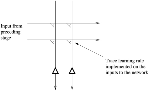
Figure 26. The learning scheme implemented in VisNet. A trace-learning rule is implemented in the feed-forward inputs to a competitive network.

In the model developed by Parga and Rolls (1998) and Elliffe et al. (2000), there is a set of inputs with fixed synaptic weights to a network. The network itself is a recurrent network, with a trace rule incorporated in the recurrent collaterals (see Figure 27). When different views of the same object are presented close together in time, the recurrent collaterals learn using the trace rule that the different views are of the same object. After learning, presentation of any of the views will cause the network to settle into an attractor that represents all the views of the object, that is which is a view-invariant representation of an object. (In this Section, the different exemplars of an object which need to be associated together are called views, for simplicity, but could at earlier stages of the hierarchy represent, for example, similar feature combinations (derived from the same object) in different positions in space.)

FIGURE 27

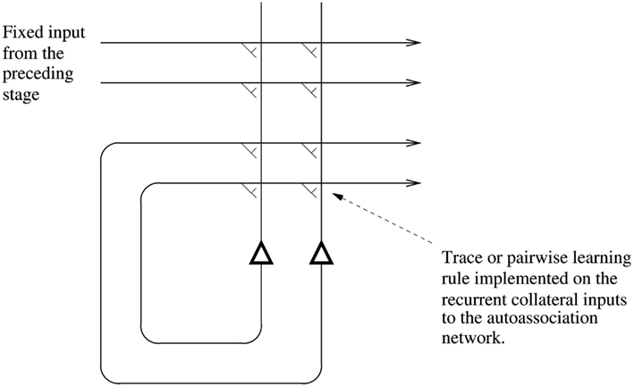
Figure 27. The learning scheme considered by Parga and Rolls (1998) and Elliffe et al. (2000). There are inputs to the network from the preceding stage via unmodifiable synapses, and a trace or pairwise associative learning rule is implemented in the recurrent collateral synapses of an autoassociative memory to associate together the different exemplars (e.g., views) of the same object.

We envisage a set of neuronal operations which set up a synaptic weight matrix in the recurrent collaterals by associating together because of their closeness in time the different views of the same object.

In more detail Parga and Rolls (1998) considered two main approaches. First, one could store in a synaptic weight matrix the s views of an object. This consists of equally associating all the views to each other, including the association of each view with itself. Choosing in Figure 28 an example such that objects are defined in terms of five different views, this might produce (if each view produced firing of one neuron at a rate of 1) a block of 5 × 5 pairs of views contributing to the synaptic efficacies each with value 1. Object 2 might produce another block of synapses of value 1 further along the diagonal, and symmetric about it. Each object or memory could then be thought of as a single attractor with a distributed representation involving five elements (each element representing a different view).

FIGURE 28

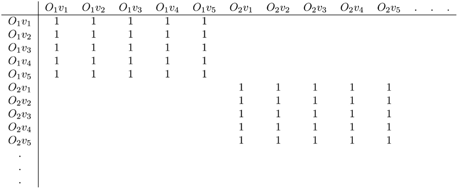
Figure 28. A schematic illustration of the first type of associations contributing to the synaptic matrix considered by Parga and Rolls (1998). Object 1 (O₁) has five views labeled v₁ to v₅, etc. The matrix is formed by associating the pattern presented in the columns with itself, that is with the same pattern presented as rows.

Then the capacity of the system in terms of the number P_o of objects that can be stored is just the number of separate attractors which can be stored in the network. For random fully distributed patterns this is as shown numerically by Hopfield (1982)

$P_o=0.14C$ (44)

where there are C inputs per neuron (and N = C neurons if the network is fully connected). Now the synaptic matrix envisaged here does not consist of random fully distributed binary elements, but instead we will assume has a sparseness a = s/N, where s is the number of views stored for each object, from any of which the whole representation of the object must be recognized. In this case, one can show (Gardner, 1988; Tsodyks and Feigel’man, 1988; Treves and Rolls, 1991) that the number of objects that can be stored and correctly retrieved is

$P_o=\frac{kC}{aln\left(1∕a\right)}$ (45)

where C is the number of synapses on each neuron devoted to the recurrent collaterals from other neurons in the network, and k is a factor that depends weakly on the detailed structure of the rate distribution, on the connectivity pattern, etc., but is approximately in the order of 0.2–0.3. A problem with this proposal is that as the number of views of each object increases to a large number (e.g., >20), the network will fail to retrieve correctly the internal representation of the object starting from any one view (which is only a fraction 1/s of the length of the stored pattern that represents an object).

The second approach, taken by Parga and Rolls (1998) and Elliffe et al. (2000), is to consider the operation of the network when the associations between pairs of views can be described by a matrix that has the general form shown in Figure 29. Such an association matrix might be produced by different views of an object appearing after a given view with equal probability, and synaptic modification occurring of the view with itself (giving rise to the diagonal term), and of any one view with that which immediately follows it.

FIGURE 29

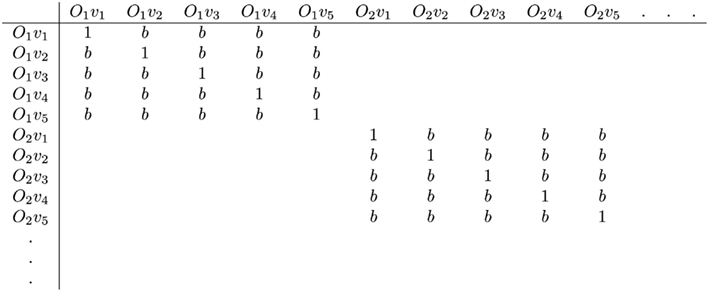
Figure 29. A schematic illustration of the second and main type of associations contributing to the synaptic matrix considered by Parga and Rolls (1998) and Elliffe et al. (2000). Object 1 (O₁) has five views labeled v₁ to v₅, etc. The association of any one view with itself has strength 1, and of any one with another view of the same object has strength b.

The same weight matrix might be produced not only by pairwise association of successive views because the association rule allows for associations over the short-time scale of, e.g., 100–200 ms, but might also be produced if the synaptic trace had an exponentially decaying form over several hundred milliseconds, allowing associations with decaying strength between views separated by one or more intervening views. The existence of a regime, for values of the coupling parameter between pairs of views in a finite interval, such that the presentation of any of the views of one object leads to the same attractor regardless of the particular view chosen as a cue, is one of the issues treated by Parga and Rolls (1998) and Elliffe et al. (2000). A related problem also dealt with was the capacity of this type of synaptic matrix: how many objects can be stored and retrieved correctly in a view-invariant way? Parga and Rolls (1998) and Elliffe et al. (2000) showed that the number grows linearly with the number of recurrent collateral connections received by each neuron. Some of the groundwork for this approach was laid by the work of Amit and collaborators (Amit, 1989; Griniasty et al., 1993).

A variant of the second approach is to consider that the remaining entries in the matrix shown in Figure 29 all have a small value. This would be produced by the fact that sometimes a view of one object would be followed by a view of a different object, when, for example, a large saccade was made, with no explicit resetting of the trace. On average, any one object would follow another rarely, and so the case is considered when all the remaining associations between pairs of views have a low value.

Parga and Rolls (1998) and Elliffe et al. (2000) were able to show that invariant object recognition is feasible in attractor neural networks in the way described. The system is able to store and retrieve in a view-invariant way an extensive number of objects, each defined by a finite set of views. What is implied by extensive is that the number of objects is proportional to the size of the network. The crucial factor that defines this size is the number of connections per neuron. In the case of the fully connected networks considered in this section, the size is thus proportional to the number of neurons. To be particular, the number of objects that can be stored is 0.081 N/5, when there are five views of each object. The number of objects is 0.073 N/11, when there are eleven views of each object. This is an interesting result in network terms, in that s views each represented by an independent random set of active neurons can, in the network described, be present in the same “object” attraction basin. It is also an interesting result in neurophysiological terms, in that the number of objects that can be represented in this network scales linearly with the number of recurrent connections per neuron. That is, the number of objects P_o that can be stored is approximately

$P_o=\frac{kC}{s}$ (46)

where C is the number of synapses on each neuron devoted to the recurrent collaterals from other neurons in the network, s is the number of views of each object, and k is a factor that is in the region of 0.07–0.09 (Parga and Rolls, 1998).

Although the explicit numerical calculation was done for a rather small number of views for each object (up to 11), the basic result, that the network can support this kind of “object” phase, is expected to hold for any number of views (the only requirement being that it does not increase with the number of neurons). This is of course enough: once an object is defined by a set of views, when the network is presented with a somewhat different stimulus or a noisy version of one of them it will still be in the attraction basin of the object attractor.

Parga and Rolls (1998) thus showed that multiple (e.g., “view”) patterns could be within the basin of attraction of a shared (e.g., “object”) representation, and that the capacity of the system was proportional to the number of synapses per neuron divided by the number of views of each object.

Elliffe et al. (2000) extended the analysis of Parga and Rolls (1998) by showing that correct retrieval could occur where retrieval “view” cues were distorted; where there was some association between the views of different objects; and where there was only partial and indeed asymmetric connectivity provided by the associatively modified recurrent collateral connections in the network. The simulations also extended the analysis by showing that the system can work well with sparse patterns, and indeed that the use of sparse patterns increases (as expected) the number of objects that can be stored in the network.

Taken together, the work described by Parga and Rolls (1998) and Elliffe et al. (2000) introduced the idea that the trace rule used to build invariant representations could be implemented in the recurrent collaterals of a neural network (as well as or as an alternative to its incorporation in the forward connections from one-layer to another incorporated in VisNet), and provided a precise analysis of the capacity of the network if it operated in this way. In the brain, it is likely that the recurrent collateral connections between cortical pyramidal cells in visual cortical areas do contribute to building invariant representations, in that if they are associatively modifiable, as seems likely, and because there is continuing firing for typically 100–300 ms after a stimulus has been shown, associations between different exemplars of the same object that occur together close in time would almost necessarily become built into the recurrent synaptic connections between pyramidal cells.

Invariant representation of faces in the context of attractor neural networks has also been discussed by Bartlett and Sejnowski (1997) in terms of a model where different views of faces are presented in a fixed sequence (Griniasty et al., 1993). This is not however the general situation; normally any pair of views can be seen consecutively and they will become associated. The model described by Parga and Rolls (1998) treats this more general situation.

I wish to note the different nature of the invariant object recognition problem studied here, and the paired associate learning task studied by Miyashita (1988), Miyashita and Chang (1988), and Sakai and Miyashita (1991). In the invariant object recognition case no particular learning protocol is required to produce an activity of the inferior temporal cortex cells responsible for invariant object recognition that is maintained for 300 ms. The learning can occur rapidly, and the learning occurs between stimuli (e.g., different views) which occur with no intervening delay. In the paired associate task, which had the aim of providing a model of semantic memory, the monkeys must learn to associate together two stimuli that are separated in time (by a number of seconds), and this type of learning can take weeks to train. During the delay period the sustained activity is rather low in the experiments, and thus the representation of the first stimulus that remains is weak, and can only poorly be associated with the second stimulus. However, formally the learning mechanism could be treated in the same way as that used by Parga and Rolls (1998) for invariant object recognition. The experimental difference is just that in the paired associate task used by Miyashita et al., it is the weak memory of the first stimulus that is associated with the second stimulus. In contrast, in the invariance learning, it would be the firing activity being produced by the first stimulus (not the weak memory of the first stimulus) that can be associated together. It is possible that the perirhinal cortex makes a useful contribution to invariant object recognition by providing a short-term memory that helps successive views of the same objects to become associated together (Buckley et al., 2001; Rolls et al., 2005a).

The mechanisms described here using an attractor network with a trace associative learning rule would apply most naturally when a small number of representations need to be associated together to represent an object. One example is associating together what is seen when an object is viewed from different perspectives. Another example is scale, with respect to which neurons early in the visual system tolerate scale changes of approximately 1.5 octaves, so that the whole scale range could be covered by associating together a limited number of such representations (see Chapter 5 of Rolls and Deco (2002) and Figure 1). The mechanism would not be so suitable when a large number of different instances would need to be associated together to form an invariant representation of objects, as might be needed for translation invariance. For the latter, the standard model of VisNet with the associative trace-learning rule implemented in the feed-forward connections (or trained by continuous spatial transformation learning as described in Section 5.10) would be more appropriate. However, both types of mechanism, with the trace rule in the feed-forward or in recurrent collateral synapses, could contribute (separately or together) to achieve invariant representations. Part of the interest of the attractor approach described in this section is that it allows analytic investigation.

Another approach to training invariance is the purely associative mechanism continuous spatial transformation learning, described in Section 5.10. With this training procedure, the capacity is increased with respect to the number of training locations, with, for example, 169 training locations producing translation-invariant representations for two face stimuli (Perry et al., 2010). When we scaled up the 32 × 32 VisNet used for most of the investigations described here to 128 × 128 neurons per layer in the VisNetL specified in Table 1, it was demonstrated that perfect translation-invariant representations were produced over at least 1,089 locations for 5 objects. Thus the indications are that scaling up the size of VisNet does markedly improve performance, and in this case allows invariant representations for 5 objects across more than 1,000 locations to be trained with continuous spatial transformation learning (Perry et al., 2010).

It will be of interest in future research to investigate how the VisNet architecture, whether trained with a trace or purely associative rule, scales up with respect to capacity as the number of neurons in the system increases further. More distributed representations in the output layer may also help to increase the capacity. In recent investigations, we have been able to train VisNetL (i.e., 128 × 128 neurons in each layer, a 256 × 256 input image, and 8 spatial frequencies for the Gabor filters as shown in Table 4) on a view-invariance learning problem, and have found good scaling up with respect to the original VisNet (i.e., 32 × 32 neurons in each layer, a 64 × 64 input image, and 4 spatial frequencies for the filters). For example, VisNetL can learn with the trace rule perfect invariant representations of 32 objects each shown in 24 views (T. J. Webb and E. T. Rolls, recent observations). The objects were made with Blender 3D modeling software, so the image views generated were carefully controlled for lighting, background intensity, etc. When trained on half of these views for each object, with the other half used for cross-validation testing, the performance was reasonable at approximately 68% correct for the 32 objects, and having the full set of 8 spatial frequencies did improve performance.

5.8. Vision in Natural Scenes – Effects of Background Versus Attention

Object-based attention refers to attention to an object. For example, in a visual search task the object might be specified as what should be searched for, and its location must be found. In spatial attention, a particular location in a scene is pre-cued, and the object at that location may need to be identified. Here we consider some of the neurophysiology of object selection and attention in the context of a feature hierarchy approach to invariant object recognition. The computational mechanisms of attention, including top-down biased competition, are described elsewhere (Rolls and Deco, 2002; Deco and Rolls, 2005b; Rolls, 2008b).

5.8.1. Neurophysiology of object selection and translation invariance in the inferior temporal visual cortex

Much of the neurophysiology, psychophysics, and modeling of attention has been with a small number, typically two, of objects in an otherwise blank scene. In this Section, I consider how attention operates in complex natural scenes, and in particular describe how the inferior temporal visual cortex operates to enable the selection of an object in a complex natural scene (see also Rolls and Deco, 2006). The inferior temporal visual cortex contains distributed and invariant representations of objects and faces (Rolls and Baylis, 1986; Hasselmo et al., 1989a; Tovee et al., 1994; Rolls and Tovee, 1995b; Rolls et al., 1997b; Booth and Rolls, 1998; Rolls, 2000, 2007a,b,c, 2011b; Rolls and Deco, 2002; Rolls and Treves, 2011).

To investigate how attention operates in complex natural scenes, and how information is passed from the inferior temporal cortex (IT) to other brain regions to enable stimuli to be selected from natural scenes for action, Rolls et al. (2003) analyzed the responses of inferior temporal cortex neurons to stimuli presented in complex natural backgrounds. The monkey had to search for two objects on a screen, and a touch of one object was rewarded with juice, and of another object was punished with saline (see Figure 3 for a schematic illustration and Figure 30 for a version of the display with examples of the stimuli shown to scale). Neuronal responses to the effective stimuli for the neurons were compared when the objects were presented in the natural scene or on a plain background. It was found that the overall response of the neuron to objects was hardly reduced when they were presented in natural scenes, and the selectivity of the neurons remained. However, the main finding was that the magnitudes of the responses of the neurons typically became much less in the real scene the further the monkey fixated in the scene away from the object (see Figure 4). A small receptive field size has also been found in inferior temporal cortex neurons when monkeys have been trained to discriminate closely spaced small visual stimuli (DiCarlo and Maunsell, 2003).

FIGURE 30

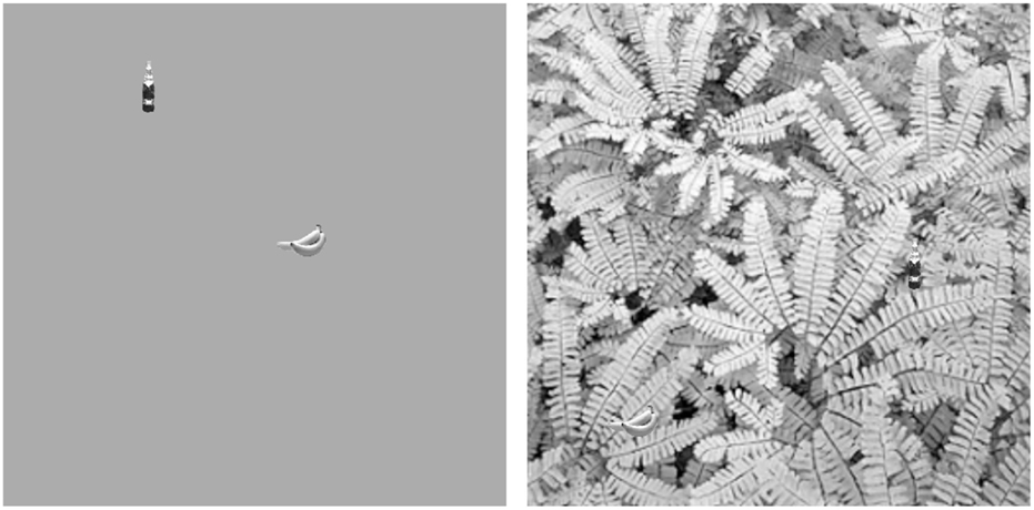
Figure 30. The visual search task. The monkey had to search for and touch an object (in this case a banana) when shown in a complex natural scene, or when shown on a plain background. In each case a second object is present (a bottle) which the monkey must not touch. The stimuli are shown to scale. The screen subtended 70° × 55° (After Rolls et al., 2003.)

It is proposed that this reduced translation invariance in natural scenes helps an unambiguous representation of an object which may be the target for action to be passed to the brain regions that receive from the primate inferior temporal visual cortex. It helps with the binding problem, by reducing in natural scenes the effective receptive field of at least some inferior temporal cortex neurons to approximately the size of an object in the scene.

It is also found that in natural scenes, the effect of object-based attention on the response properties of inferior temporal cortex neurons is relatively small, as illustrated in Figure 31 (Rolls et al., 2003).

FIGURE 31

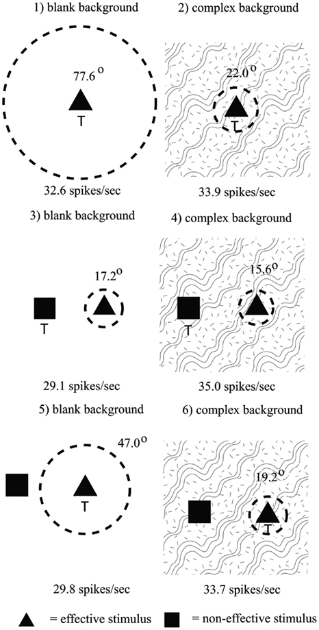
Figure 31. Summary of the receptive field sizes of inferior temporal cortex neurons to a 5° effective stimulus presented in either a blank background (blank screen) or in a natural scene (complex background). The stimulus that was a target for action in the different experimental conditions is marked by T. When the target stimulus was touched, a reward was obtained. The mean receptive field diameter of the population of neurons analyzed, and the mean firing rate in spikes/s, is shown. The stimuli subtended 5° × 3.5° at the retina, and occurred on each trial in a random position in the 70° × 55° screen. The dashed circle is proportional to the receptive field size. Top row: responses with one visual stimulus in a blank (left) or complex (right) background. Middle row: responses with two stimuli, when the effective stimulus was not the target of the visual search. Bottom row: responses with two stimuli, when the effective stimulus was the target of the visual search. (After Rolls et al., 2003.)

5.8.2. Attention and translation invariance in natural scenes – a computational account

The results summarized in Figure 31 for 5° stimuli show that the receptive fields were large (77.6°) with a single stimulus in a blank background (top left), and were greatly reduced in size (to 22.0°) when presented in a complex natural scene (top right). The results also show that there was little difference in receptive field size or firing rate in the complex background when the effective stimulus was selected for action (bottom right, 19.2°), and when it was not (middle right, 15.6°; Rolls et al., 2003). (For comparison, the effects of attention against a blank background were much larger, with the receptive field increasing from 17.2° to 47.0° as a result of object-based attention, as shown in Figure 31, left middle and bottom.)

Trappenberg et al. (2002) have suggested what underlying mechanisms could account for these findings, and simulated a model to test the ideas. The model utilizes an attractor network representing the inferior temporal visual cortex (implemented by the recurrent connections between inferior temporal cortex neurons), and a neural input layer with several retinotopically organized modules representing the visual scene in an earlier visual cortical area such as V4 (see Figure 32). The attractor network aspect of the model produces the property that the receptive fields of IT neurons can be large in blank scenes by enabling a weak input in the periphery of the visual field to act as a retrieval cue for the object attractor. On the other hand, when the object is shown in a complex background, the object closest to the fovea tends to act as the retrieval cue for the attractor, because the fovea is given increased weight in activating the IT module because the magnitude of the input activity from objects at the fovea is greatest due to the higher magnification factor of the fovea incorporated into the model. This results in smaller receptive fields of IT neurons in complex scenes, because the object tends to need to be close to the fovea to trigger the attractor into the state representing that object. (In other words, if the object is far from the fovea, then it will not trigger neurons in IT which represent it, because neurons in IT are preferentially being activated by another object at the fovea.) This may be described as an attractor model in which the competition for which attractor state is retrieved is weighted toward objects at the fovea.

FIGURE 32

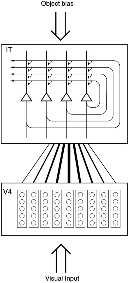
Figure 32. The architecture of the inferior temporal cortex (IT) model of Trappenberg et al. (2002) operating as an attractor network with inputs from the fovea given preferential weighting by the greater magnification factor of the fovea. The model also has a top-down object-selective bias input. The model was used to analyze how object vision and recognition operate in complex natural scenes.

Attentional top-down object-based inputs can bias the competition implemented in this attractor model, but have relatively minor effects (in, for example, increasing receptive field size) when they are applied in a complex natural scene, as then as usual the stronger forward inputs dominate the states reached. In this network, the recurrent collateral connections may be thought of as implementing constraints between the different inputs present, to help arrive at firing in the network which best meets the constraints. In this scenario, the preferential weighting of objects close to the fovea because of the increased magnification factor at the fovea is a useful principle in enabling the system to provide useful output. The attentional object biasing effect is much more marked in a blank scene, or a scene with only two objects present at similar distances from the fovea, which are conditions in which attentional effects have frequently been examined. The results of the investigation (Trappenberg et al., 2002) thus suggest that top-down attention may be a much more limited phenomenon in complex, natural, scenes than in reduced displays with one or two objects present. The results also suggest that the alternative principle, of providing strong weight to whatever is close to the fovea, is an important principle governing the operation of the inferior temporal visual cortex, and in general of the output of the visual system in natural environments. This principle of operation is very important in interfacing the visual system to action systems, because the effective stimulus in making inferior temporal cortex neurons fire is in natural scenes usually on or close to the fovea. This means that the spatial coordinates of where the object is in the scene do not have to be represented in the inferior temporal visual cortex, nor passed from it to the action selection system, as the latter can assume that the object making IT neurons fire is close to the fovea in natural scenes.

There may of course be in addition a mechanism for object selection that takes into account the locus of covert attention when actions are made to locations not being looked at. However, the simulations described in this section suggest that in any case covert attention is likely to be a much less significant influence on visual processing in natural scenes than in reduced scenes with one or two objects present.

Given these points, one might question why inferior temporal cortex neurons can have such large receptive fields, which show translation invariance. At least part of the answer to this may be that inferior temporal cortex neurons must have the capability to be large if they are to deal with large objects. A V1 neuron, with its small receptive field, simply could not receive input from all the features necessary to define an object. On the other hand, inferior temporal cortex neurons may be able to adjust their size to approximately the size of objects, using in part the interactive effects involved in attention (Rolls, 2008b), and need the capability for translation invariance because the actual relative positions of the features of an object could be at different relative positions in the scene. For example, a car can be recognized whichever way it is viewed, so that the parts (such as the bonnet or hood) must be identifiable as parts wherever they happen to be in the image, though of course the parts themselves also have to be in the correct relative positions, as allowed for by the hierarchical feature analysis architecture described in this paper.

Some details of the simulations follow. Each independent module within “V4” in Figure 32 represents a small part of the visual field and receives input from earlier visual areas represented by an input vector for each possible location which is unique for each object. Each module was 6° in width, matching the size of the objects presented to the network. For the simulations Trappenberg et al. (2002) chose binary random input vectors representing objects with N^V4a^V4 components set to ones and the remaining N^V4(1 − a^V4) components set to zeros. N^V4 is the number of nodes in each module and a^V4 is the sparseness of the representation which was set to be a^V4 = 0.2 in the simulations.

The structure labeled “IT” represents areas of visual association cortex such as the inferior temporal visual cortex and cortex in the anterior part of the superior temporal sulcus in which neurons provide distributed representations of faces and objects (Booth and Rolls, 1998; Rolls, 2000). Nodes in this structure are governed by leaky integrator dynamics with time constant τ

$\begin{array}{rcll}\tau \frac{d{h}_i^{\text{IT}}\left(t\right)}{dt}& =-h_i^{\text{IT}}\left(t\right)+\sum _j\left(w_{ij}^{\text{IT}}-c^{\text{IT}}\right)y_j^{\text{IT}}\left(t\right)& & \\ & +\sum _k{w}_{ik}^{\text{IT}-\text{V}4}{y}_k^{\text{V}4}\left(t\right)+k^{\text{IT\_BIAS}}{I}_i^{\text{OBJ}}.& & \text{(47)}\end{array}$

The firing rate $y_i^{\text{IT}}$ of the ith node is determined by a sigmoidal function from the activation $h_i^{\text{IT}}$ as follows

$y_i^{\text{IT}}\left(t\right)=\frac{1}{1+exp\left[-2\beta \left(h_i^{\text{IT}}\left(t\right)-\alpha \right)\right]},$ (48)

where the parameters β = 1 and α = 1 represent the gain and the bias, respectively.

The recognition functionality of this structure is modeled as an attractor neural network (ANN) with trained memories indexed by μ representing particular objects. The memories are formed through Hebbian learning on sparse patterns,

$w_{ij}^{\text{IT}}=k^{\text{IT}}\sum _{\mu }\left({\xi }_i^{\mu }-a^{IT}\right)\left({\xi }_j^{\mu }-a^{IT}\right),$ (49)

where k^IT (set to 1 in the simulations) is a normalization constant that depends on the learning rate, a^IT = 0.2 is the sparseness of the training pattern in IT, and ${\xi }_i^{\mu }$ are the components of the pattern used to train the network. The constant c^IT in equation (47) represents the strength of the activity-dependent global inhibition simulating the effects of inhibitory interneurons. The external “top-down” input vector I^OBJ produces object-selective inputs, which are used as the attentional drive when a visual search task is simulated. The strength of this object bias is modulated by the value of k^IT_BIAS in equation (47).

The weights $w_{ij}^{\text{IT}-\text{V}4}$ between the V4 nodes and IT nodes were trained by Hebbian learning of the form

$w_{ij}^{\text{IT}-\text{V}4}=k^{\text{IT}-\text{V}4}\left(k\right)\sum _{\mu }\left({\xi }_i^{\mu }-a^{V4}\right)\left({\xi }_j^{\mu }-a^{IT}\right).$ (50)

to produce object representations in IT based on inputs in V4. The normalizing modulation factor k^IT−V4(k) allows the gain of inputs to be modulated as a function of their distance from the fovea, and depends on the module k to which the presynaptic node belongs. The model supports translation-invariant object recognition of a single object in the visual field if the normalization factor is the same for each module and the model is trained with the objects placed at every possible location in the visual field. The translation invariance of the weight vectors between each “V4” module and the IT nodes is however explicitly modulated in the model by the module-dependent modulation factor k^IT−V4(k) as indicated in Figure 32 by the width of the lines connecting V4 with IT. The strength of the foveal V4 module is strongest, and the strength decreases for modules representing increasing eccentricity. The form of this modulation factor was derived from the parameterization of the cortical magnification factors given by Dow et al. (1981).

To study the ability of the model to recognize trained objects at various locations relative to the fovea the system was trained on a set of objects. The network was then tested with distorted versions of the objects, and the “correlation” between the target object and the final state of the attractor network was taken as a measure of the performance. The correlation was estimated from the normalized dot product between the target object vector that was used during training the IT network, and the state of the IT network after a fixed amount of time sufficient for the network to settle into a stable state. The objects were always presented on backgrounds with some noise (introduced by flipping 2% of the bits in the scene which were not the test stimulus) in order to utilize the properties of the attractor network, and because the input to IT will inevitably be noisy under normal conditions of operation.

In the first simulation only one object was present in the visual scene in a plain (blank) background at different eccentricities from the fovea. As shown in Figure 33A by the line labeled “blank background,” the receptive fields of the neurons were very large. The value of the object bias k^IT_BIAS was set to 0 in these simulations. Good object retrieval (indicated by large correlations) was found even when the object was far from the fovea, indicating large IT receptive fields with a blank background. The reason that any drop is seen in performance as a function of eccentricity is because flipping 2% of the bits outside the object introduces some noise into the recall process. This demonstrates that the attractor dynamics can support translation-invariant object recognition even though the translation-invariant weight vectors between V4 and IT are explicitly modulated by the modulation factor k^IT−V4 derived from the cortical magnification factor.

FIGURE 33

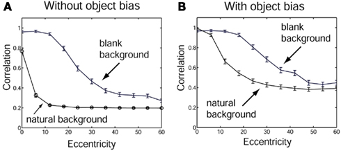
Figure 33. Correlations as measured by the normalized dot product between the object vector used to train IT and the state of the IT network after settling into a stable state with a single object in the visual scene (blank background) or with other trained objects at all possible locations in the visual scene (natural background). There is no object bias included in the results shown in graph (A), whereas an object bias is included in the results shown in (B) with k^IT_BIAS = 0.7 in the experiments with a natural background and k^IT_BIAS = 0.1 in the experiments with a blank background. (After Trappenberg et al., 2002.)

In a second simulation individual objects were placed at all possible locations in a natural and cluttered visual scene. The resulting correlations between the target pattern and the asymptotic IT state are shown in Figure 33A with the line labeled “natural background.” Many objects in the visual scene are now competing for recognition by the attractor network, and the objects around the foveal position are enhanced through the modulation factor derived from the cortical magnification factor. This results in a much smaller size of the receptive field of IT neurons when measured with objects in natural backgrounds.

In addition to this major effect of the background on the size of the receptive field, which parallels and may account for the physiological findings outlined above and in Section 5.8.1, there is also a dependence of the size of the receptive fields on the level of object bias provided to the IT network. Examples are shown in Figure 33B where an object bias was used. The object bias biases the IT network toward the expected object with a strength determined by the value of k^IT−BIAS, and has the effect of increasing the size of the receptive fields in both blank and natural backgrounds (see Figure 33B compared to Figure 33A). This models the effect found neurophysiologically (Rolls et al., 2003).

Some of the conclusions are as follows (Trappenberg et al., 2002). When single objects are shown in a scene with a blank background, the attractor network helps neurons to respond to an object with large eccentricities of this object relative to the fovea of the agent. When the object is presented in a natural scene, other neurons in the inferior temporal cortex become activated by the other effective stimuli present in the visual field, and these forward inputs decrease the response of the network to the target stimulus by a competitive process. The results found fit well with the neurophysiological data, in that IT operates with almost complete translation invariance when there is only one object in the scene, and reduces the receptive field size of its neurons when the object is presented in a cluttered environment. The model described here provides an explanation of the responses of real IT neurons in natural scenes.

In natural scenes, the model is able to account for the neurophysiological data that the IT neuronal responses are larger when the object is close to the fovea, by virtue of fact that objects close to the fovea are weighted by the cortical magnification factor related modulation k^IT−V4.

The model accounts for the larger receptive field sizes from the fovea of IT neurons in natural backgrounds if the target is the object being selected compared to when it is not selected (Rolls et al., 2003). The model accounts for this by an effect of top-down bias which simply biases the neurons toward particular objects compensating for their decreasing inputs produced by the decreasing magnification factor modulation with increasing distance from the fovea. Such object-based attention signals could originate in the prefrontal cortex and could provide the object bias for the inferior temporal visual cortex (Renart et al., 2000; Rolls, 2008b).

Important properties of the architecture for obtaining the results just described are the high magnification factor at the fovea and the competition between the effects of different inputs, implemented in the above simulation by the competition inherent in an attractor network.

We have also been able to obtain similar results in a hierarchical feed-forward network where each layer operates as a competitive network (Deco and Rolls, 2004). This network thus captures many of the properties of our hierarchical model of invariant object recognition (Rolls, 1992; Wallis and Rolls, 1997; Rolls and Milward, 2000; Stringer and Rolls, 2000, 2002; Rolls and Stringer, 2001, 2006, 2007; Elliffe et al., 2002; Rolls and Deco, 2002; Stringer et al., 2006), but incorporates in addition a foveal magnification factor and top-down projections with a dorsal visual stream so that attentional effects can be studied, as shown in Figure 34.

FIGURE 34

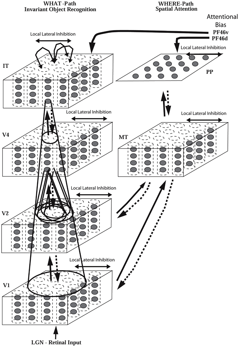
Figure 34. Cortical architecture for hierarchical and attention-based visual perception after Deco and Rolls (2004). The system is essentially composed of five modules structured such that they resemble the two known main visual paths of the mammalian visual cortex. Information from the retino-geniculo-striate pathway enters the visual cortex through area V1 in the occipital lobe and proceeds into two processing streams. The occipital-temporal stream leads ventrally through V2–V4 and IT (inferior temporal visual cortex), and is mainly concerned with object recognition. The occipito-parietal stream leads dorsally into PP (posterior parietal complex), and is responsible for maintaining a spatial map of an object’s location. The solid lines with arrows between levels show the forward connections, and the dashed lines the top-down backprojections. Short-term memory systems in the prefrontal cortex (PF46) apply top-down attentional bias to the object or spatial processing streams. (After Deco and Rolls, 2004.)

Deco and Rolls (2004) trained the network shown in Figure 34 with two objects, and used the trace-learning rule (Wallis and Rolls, 1997; Rolls and Milward, 2000) in order to achieve translation invariance. In a first experiment we placed only one object on the retina at different distances from the fovea (i.e., different eccentricities relative to the fovea). This corresponds to the blank background condition. In a second experiment, we also placed the object at different eccentricities relative to the fovea, but on a cluttered natural background. Larger receptive fields were found with the blank as compared to the cluttered natural background.

Deco and Rolls (2004) also studied the influence of object-based attentional top-down bias on the effective size of the receptive field of an inferior temporal cortex neuron for the case of an object in a blank or a cluttered background. To do this, they repeated the two simulations but now considered a non-zero top-down bias coming from prefrontal area 46v and impinging on the inferior temporal cortex neuron specific for the object tested. When no attentional object bias was introduced, a shrinkage of the receptive field size was observed in the complex vs the blank background. When attentional object bias was introduced, the shrinkage of the receptive field due to the complex background was somewhat reduced. This is consistent with the neurophysiological results (Rolls et al., 2003). In the framework of the model (Deco and Rolls, 2004), the reduction of the shrinkage of the receptive field is due to the biasing of the competition in the inferior temporal cortex layer in favor of the specific IT neuron tested, so that it shows more translation invariance (i.e., a slightly larger receptive field). The increase of the receptive field size of an IT neuron, although small, produced by the external top-down attentional bias offers a mechanism for facilitation of the search for specific objects in complex natural scenes (Rolls, 2008b).

I note that it is possible that a “spotlight of attention” (Desimone and Duncan, 1995) can be moved covertly away from the fovea (Rolls, 2008b). However, at least during normal visual search tasks in natural scenes, the neurons are sensitive to the object at which the monkey is looking, that is primarily to the object that is on the fovea, as shown by Rolls et al. (2003) and Aggelopoulos and Rolls (2005), and described in Sections 1 and 9.

5.9. The Representation of Multiple Objects in a Scene

When objects have distributed representations, there is a problem of how multiple objects (whether the same or different) can be represented in a scene, because the distributed representations overlap, and it may not be possible to determine whether one has an amalgam of several objects, or a new object (Mozer, 1991), or multiple instances of the same object, let alone the relative spatial positions of the objects in a scene. Yet humans can determine the relative spatial locations of objects in a scene even in short presentation times without eye movements (Biederman, 1972; and this has been held to involve some spotlight of attention). Aggelopoulos and Rolls (2005) analyzed this issue by recording from single inferior temporal cortex neurons with five objects simultaneously present in the receptive field. They found that although all the neurons responded to their effective stimulus when it was at the fovea, some could also respond to their effective stimulus when it was in some but not other parafoveal positions 10° from the fovea. An example of such a neuron is shown in Figure 35. The asymmetry is much more evident in a scene with 5 images present (Figure 35A) than when only one image is shown on an otherwise blank screen (Figure 35B). Competition between different stimuli in the receptive field thus reveals the asymmetry in the receptive field of inferior temporal visual cortex neurons.

FIGURE 35

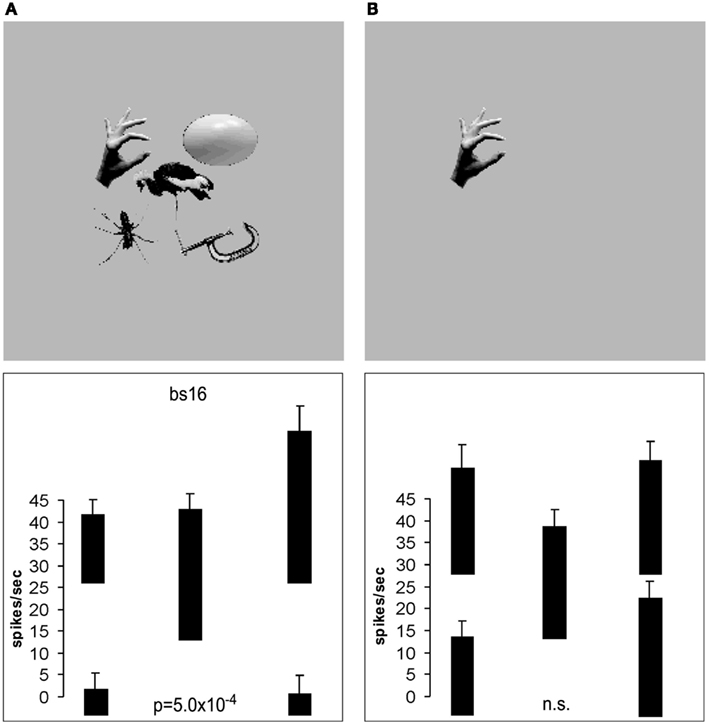
Figure 35. (A) The responses (firing rate with the spontaneous rate subtracted, means ± sem) of an inferior temporal cortex neuron when tested with 5 stimuli simultaneously present in the close (10°) configuration with the parafoveal stimuli located 10° from the fovea. (B) The responses of the same neuron when only the effective stimulus was presented in each position. The firing rate for each position is that when the effective stimulus (in this case the hand) for the neuron was in that position. The p value is that from the ANOVA calculated over the four parafoveal positions. (After Aggelopoulos and Rolls, 2005.)

The asymmetry provides a way of encoding the position of multiple objects in a scene. Depending on which asymmetric neurons are firing, the population of neurons provides information to the next processing stage not only about which image is present at or close to the fovea, but where it is with respect to the fovea.

Simulations with VisNet with an added layer to simulate hippocampal scene memory have demonstrated that receptive field asymmetry appears when multiple objects are simultaneously present because of the probabilistic connectivity from the preceding stage which introduces asymmetry, which becomes revealed by the enhanced lateral inhibition when multiple objects are presented simultaneously (Rolls et al., 2008).

The information in the inferior temporal visual cortex is provided by neurons that have firing rates that reflect the relevant information, and stimulus-dependent synchrony is not necessary (Aggelopoulos and Rolls, 2005). Top-down attentional biasing input could thus, by biasing the appropriate neurons, facilitate bottom-up information about objects without any need to alter the time relations between the firing of different neurons. The exact position of the object with respect to the fovea, and effectively thus its spatial position relative to other objects in the scene, would then be made evident by the subset of asymmetric neurons firing.

This is thus the solution that these experiments (Aggelopoulos and Rolls, 2005; Rolls et al., 2008) indicate is used for the representation of multiple objects in a scene, an issue that has previously been difficult to account for in neural systems with distributed representations (Mozer, 1991) and for which “attention” has been a proposed solution.

The learning of invariant representations of objects when multiple objects are present in a scene is considered in Section 5.5.2.

5.10. Learning Invariant Representations Using Spatial Continuity: Continuous Spatial Transformation Learning

The temporal continuity typical of objects has been used in an associative learning rule with a short-term memory trace to help build invariant object representations in the networks described previously in this paper. Stringer et al. (2006) showed that spatial continuity can also provide a basis for helping a system to self-organize invariant representations. They introduced a new learning paradigm “continuous spatial transformation (CT) learning” which operates by mapping spatially similar input patterns to the same post-synaptic neurons in a competitive learning system. As the inputs move through the space of possible continuous transforms (e.g., translation, rotation, etc.), the active synapses are modified onto the set of post-synaptic neurons. Because other transforms of the same stimulus overlap with previously learned exemplars, a common set of post-synaptic neurons is activated by the new transforms, and learning of the new active inputs onto the same post-synaptic neurons is facilitated.

The concept is illustrated in Figure 36. During the presentation of a visual image at one position on the retina that activates neurons in layer 1, a small winning set of neurons in layer 2 will modify (through associative learning) their afferent connections from layer 1 to respond well to that image in that location. When the same image appears later at nearby locations, so that there is spatial continuity, the same neurons in layer 2 will be activated because some of the active afferents are the same as when the image was in the first position. The key point is that if these afferent connections have been strengthened sufficiently while the image is in the first location, then these connections will be able to continue to activate the same neurons in layer 2 when the image appears in overlapping nearby locations. Thus the same neurons in the output layer have learned to respond to inputs that have similar vector elements in common.

FIGURE 36

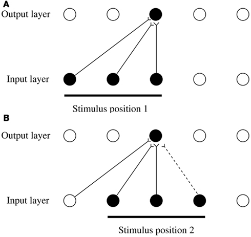
Figure 36. An illustration of how continuous spatial transformation (CT) learning would function in a network with a single-layer of forward synaptic connections between an input layer of neurons and an output layer. Initially the forward synaptic weights are set to random values. The top part (A) shows the initial presentation of a stimulus to the network in position 1. Activation from the (shaded) active input cells is transmitted through the initially random forward connections to stimulate the cells in the output layer. The shaded cell in the output layer wins the competition in that layer. The weights from the active input cells to the active output neuron are then strengthened using an associative learning rule. The bottom part (B) shows what happens after the stimulus is shifted by a small amount to a new partially overlapping position 2. As some of the active input cells are the same as those that were active when the stimulus was presented in position 1, the same output cell is driven by these previously strengthened afferents to win the competition again. The rightmost shaded input cell activated by the stimulus in position 2, which was inactive when the stimulus was in position 1, now has its connection to the active output cell strengthened (denoted by the dashed line). Thus the same neuron in the output layer has learned to respond to the two input patterns that have similar vector elements in common. As can be seen, the process can be continued for subsequent shifts, provided that a sufficient proportion of input cells stay active between individual shifts. (After Stringer et al., 2006.)

As can be seen in Figure 36, the process can be continued for subsequent shifts, provided that a sufficient proportion of input cells stay active between individual shifts. This whole process is repeated throughout the network, both horizontally as the image moves on the retina, and hierarchically up through the network. Over a series of stages, transform invariant (e.g., location invariant) representations of images are successfully learned, allowing the network to perform invariant object recognition. A similar CT learning process may operate for other kinds of transformation, such as change in view or size.

Stringer et al. (2006) demonstrated that VisNet can be trained with continuous spatial transformation learning to form view-invariant representations. They showed that CT learning requires the training transforms to be relatively close together spatially so that spatial continuity is present in the training set; and that the order of stimulus presentation is not crucial, with even interleaving with other objects possible during training, because it is spatial continuity rather the temporal continuity that drives the self-organizing learning with the purely associative synaptic modification rule.

Perry et al. (2006) extended these simulations with VisNet of view-invariant learning using CT to more complex 3D objects, and using the same training images in human psychophysical investigations, showed that view-invariant object learning can occur when spatial but not temporal continuity applies in a training condition in which the images of different objects were interleaved. However, they also found that the human view-invariance learning was better if sequential presentation of the images of an object was used, indicating that temporal continuity is an important factor in human invariance learning.

Perry et al. (2010) extended the use of continuous spatial transformation learning to translation invariance. They showed that translation-invariant representations can be learned by continuous spatial transformation learning; that the transforms must be close for this to occur; that the temporal order of presentation of each transformed image during training is not crucial for learning to occur; that relatively large numbers of transforms can be learned; and that such continuous spatial transformation learning can be usefully combined with temporal trace training.

5.11. Lighting Invariance

Object recognition should occur correctly even despite variations of lighting. In an investigation of this, Rolls and Stringer (2006) trained VisNet on a set of 3D objects generated with OpenGL in which the viewing angle and lighting source could be independently varied (see Figure 37). After training with the trace rule on all the 180 views (separated by 1°, and rotated about the vertical axis in Figure 37) of each of the four objects under the left lighting condition, we tested whether the network would recognize the objects correctly when they were shown again, but with the source of the lighting moved to the right so that the objects appeared different (see Figure 37). With this protocol, lighting invariant object recognition by VisNet was demonstrated (Rolls and Stringer, 2006).

FIGURE 37

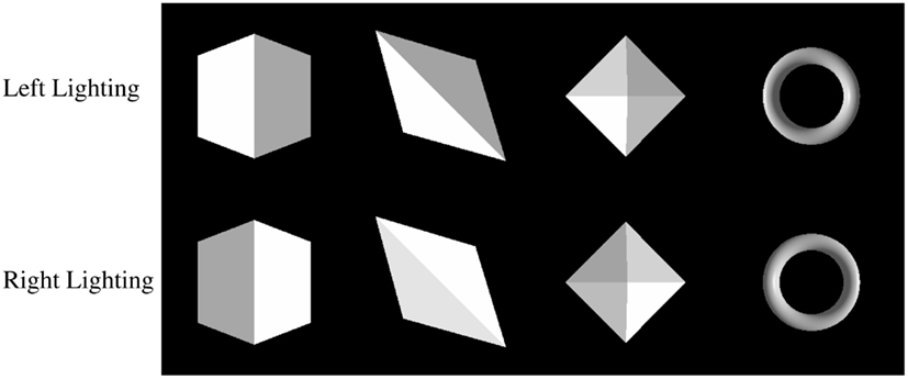
Figure 37. Lighting invariance. VisNet was trained on a set of 3D objects (cube, tetrahedron, octahedron, and torus) generated with OpenGL in which for training the objects had left lighting, and for testing the objects had right lighting. Just one view of each object is shown in the Figure, but for training and testing 180 views of each object separated by 1° were used. (After Rolls and Stringer, 2006.)

Some insight into the good performance with a change of lighting is that some neurons in the inferior temporal visual cortex respond to the outlines of 3D objects (Vogels and Biederman, 2002), and these outlines will be relatively consistent across lighting variations. Although the features about the object represented in VisNet will include more than the representations of the outlines, the network may because it uses distributed representations of each object generalize correctly provided that some of the features are similar to those present during training. Under very difficult lighting conditions, it is likely that the performance of the network could be improved by including variations in the lighting during training, so that the trace rule could help to build representations that are explicitly invariant with respect to lighting.

5.12. Invariant Global Motion in the Dorsal Visual System

A key issue in understanding the cortical mechanisms that underlie motion perception is how we perceive the motion of objects such as a rotating wheel invariantly with respect to position on the retina, and size. For example, we perceive the wheel shown in Figure 38A rotating clockwise independently of its position on the retina. This occurs even though the local motion for the wheels in the different positions may be opposite. How could this invariance of the visual motion perception of objects arise in the visual system? Invariant motion representations are known to be developed in the cortical dorsal visual system. Motion-sensitive neurons in V1 have small receptive fields (in the range 1–2° at the fovea), and can therefore not detect global motion, and this is part of the aperture problem (Wurtz and Kandel, 2000b). Neurons in MT, which receives inputs from V1 and V2, have larger receptive fields (e.g., 5° at the fovea), and are able to respond to planar global motion, such as a field of small dots in which the majority (in practice as few as 55%) move in one direction, or to the overall direction of a moving plaid, the orthogonal grating components of which have motion at 45° to the overall motion (Movshon et al., 1985; Newsome et al., 1989). Further on in the dorsal visual system, some neurons in macaque visual area MST (but not MT) respond to rotating flow fields or looming with considerable translation invariance (Graziano et al., 1994; Geesaman and Andersen, 1996). In the cortex in the anterior part of the superior temporal sulcus, which is a convergence zone for inputs from the ventral and dorsal visual systems, some neurons respond to object-based motion, for example, to a head rotating clockwise but not anticlockwise, independently of whether the head is upright or inverted which reverses the optic flow across the retina (Hasselmo et al., 1989b).

FIGURE 38

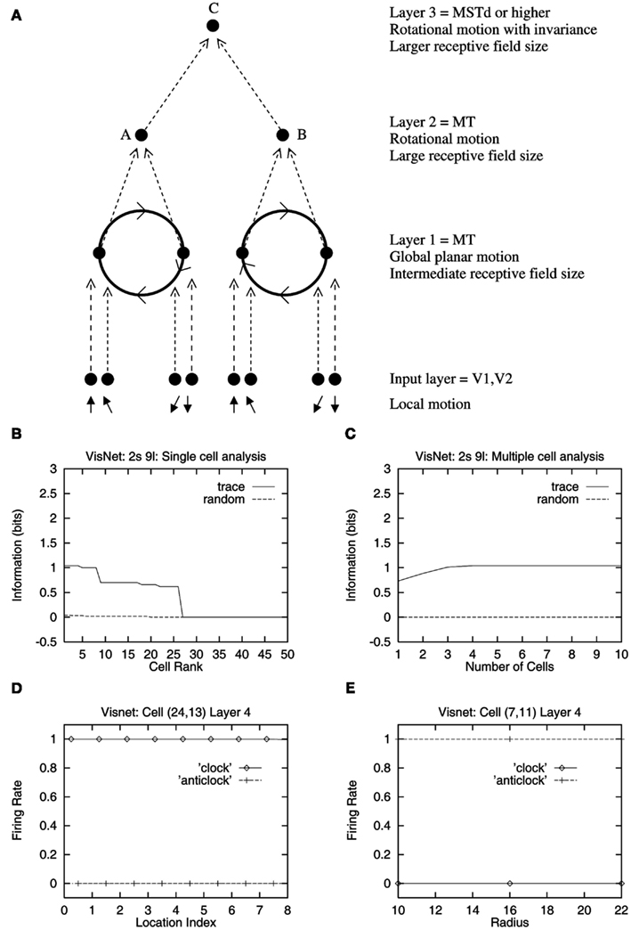
Figure 38. (A) Two rotating wheels at different locations rotating in opposite directions. The local flow field is ambiguous. Clockwise or counterclockwise rotation can only be diagnosed by a global flow computation, and it is shown how the network is expected to solve the problem to produce position-invariant global motion-sensitive neurons. One rotating wheel is presented at any one time, but the need is to develop a representation of the fact that in the case shown the rotating flow field is always clockwise, independently of the location of the flow field. (B–D) Translation invariance, with training on 9 locations. (B) Single cell information measures showing that some layer 4 neurons have perfect performance of 1 bit (clockwise vs anticlockwise) after training with the trace rule, but not with random initial synaptic weights in the untrained control condition. (C) The multiple cell information measure shows that small groups of neurons have perfect performance. (D) Position invariance illustrated for a single cell from layer 4, which responded only to the clockwise rotation, and for every one of the 9 positions. (E) Size-invariance illustrated for a single cell from layer 4, which after training with three different radii of rotating wheel, responded only to anticlockwise rotation, independently of the size of the rotating wheels. (After Rolls and Stringer, 2007.)

In a unifying hypothesis with the design of the ventral cortical visual system Rolls and Stringer (2007) proposed that the dorsal visual system uses a hierarchical feed-forward network architecture (V1, V2, MT, MSTd, parietal cortex) with training of the connections with a short-term memory trace associative synaptic modification rule to capture what is invariant at each stage. The principle is illustrated in Figure 38A. Simulations showed that the proposal is computationally feasible, in that invariant representations of the motion flow fields produced by objects self-organize in the later layers of the architecture (see examples in Figures 38B–E). The model produces invariant representations of the motion flow fields produced by global in-plane motion of an object, in-plane rotational motion, looming vs receding of the object. The model also produces invariant representations of object-based rotation about a principal axis. Thus it is proposed that the dorsal and ventral visual systems may share some unifying computational principles Rolls and Stringer (2007). Indeed, the simulations of Rolls and Stringer (2007) used a standard version of VisNet, with the exception that instead of using oriented bar receptive fields as the input to the first layer, local motion flow fields provided the inputs.

6. Learning Invariant Representations of Scenes and Places

The primate hippocampal system has neurons that respond to a view of a spatial scene, or when that location in a scene is being looked at in the dark or when it is obscured (Rolls et al., 1997a, 1998; Robertson et al., 1998; Georges-François et al., 1999; Rolls and Xiang, 2006; Rolls, 2008b). The representation is relatively invariant with respect to the position of the macaque in the environment, and of head direction, and eye position. The requirement for these spatial view neurons is that a position in the spatial scene is being looked at. (There is an analogous set of place neurons in the rat hippocampus that respond in this case when the rat is in a given position in space, relatively invariantly with respect to head direction (McNaughton et al., 1983; O’Keefe, 1984; Muller et al., 1991).) How might these spatial view neurons be set up in primates?

Before addressing this, it is useful to consider the difference between a spatial view or scene representation, and an object representation. An object can be moved to different places in space or in a spatial scene. An example is a motor car that can be moved to different places in space. The object is defined by a combination of features or parts in the correct relative spatial position, but its representation is independent of where it is in space. In contrast, a representation of space has objects in defined relative spatial positions, which cannot be moved relative to one another in space. An example might be Trafalgar Square, in which Nelson’s column is in the middle, and the National Gallery and St Martin’s in the Fields church are at set relative locations in space, and cannot be moved relative to one another. This draws out the point that there may be some computational similarities between the construction of an objects and of a scene or a representation of space, but there are also important differences in how they are used. In the present context we are interested in how the brain may set up a spatial view representation in which the relative position of the objects in the scene defines the spatial view. That spatial view representation may be relatively invariant with respect to the exact position from which the scene is viewed (though extensions are needed if there are central objects in a space through which one moves).

It is now possible to propose a unifying hypothesis of the relation between the ventral visual system, and primate hippocampal spatial view representations (Rolls, 2008b; Rolls et al., 2008). Let us consider a computational architecture in which a fifth layer is added to the VisNet architecture, as illustrated in Figure 39. In the anterior inferior temporal visual cortex, which corresponds to the fourth layer of VisNet, neurons respond to objects, but several objects close to the fovea (within approximately 10°) can be represented because many object-tuned neurons have asymmetric receptive fields with respect to the fovea (Aggelopoulos and Rolls, 2005; see Section 5.9). If the fifth layer of VisNet performs the same operation as previous layers, it will form neurons that respond to combinations of objects in the scene with the positions of the objects relative spatially to each other incorporated into the representation (as described in Section 5.4). The result will be spatial view neurons in the case of primates when the visual field of the primate has a narrow focus (due to the high-resolution fovea), and place cells when as in the rat the visual field is very wide (De Araujo et al., 2001; Rolls, 2008b). The trace-learning rule in layer 5 should help the spatial view or place fields that develop to be large and single, because of the temporal continuity that is inherent when the agent moves from one part of the view or place space to another, in the same way as has been shown for the entorhinal grid cell to hippocampal place cell mapping (Rolls et al., 2006b; Rolls, 2008b).

FIGURE 39

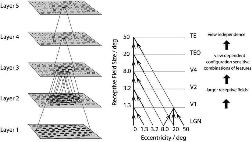
Figure 39. Adding a fifth layer, corresponding to the parahippocampal gyrus/hippocampal system, after the inferior temporal visual cortex (corresponding to layer 4) may lead to the self-organization of spatial view/place cells in layer 5 when whole scenes are presented (see text). Convergence in the visual system is shown in the earlier layers. Right – as it occurs in the brain. V1, visual cortex area V1; TEO, posterior inferior temporal cortex; TE, inferior temporal cortex (IT). Left – as implemented in VisNet (layers 1–4). Convergence through the network is designed to provide fourth layer neurons with information from across the entire input retina.

The hippocampal dentate granule cells form a network expected to be important in this competitive learning of spatial view or place representations based on visual inputs. As the animal navigates through the environment, different spatial view cells would be formed. Because of the overlapping fields of adjacent spatial view neurons, and hence their coactivity as the animal navigates, recurrent collateral associative connections at the next stage of the system, CA3, could form a continuous attractor representation of the environment (Rolls, 2008b). We thus have a hypothesis for how the spatial representations are formed as a natural extension of the hierarchically organized competitive networks in the ventral visual system. The expression of such spatial representations in CA3 may be particularly useful for associating those spatial representations with other inputs, such as objects or rewards (Rolls, 2008b).

We have performed simulations to test this hypothesis with VisNet simulations with conceptually a fifth layer added (Rolls et al., 2008). Training now with whole scenes that consist of a set of objects in a given fixed spatial relation to each other results in neurons in the added layer that respond to one of the trained whole scenes, but do not respond if the objects in the scene are rearranged to make a new scene from the same objects. The formation of these scene-specific representations in the added layer is related to the fact that in the inferior temporal cortex (Aggelopoulos and Rolls, 2005), and in the VisNet model (Rolls et al., 2008), the receptive fields of inferior temporal cortex neurons shrink and become asymmetric when multiple objects are present simultaneously in a natural scene. This also provides a solution to the issue of the representation of multiple objects, and their relative spatial positions, in complex natural scenes (Rolls, 2008b).

Consistently, in a more artificial network trained by gradient ascent with a goal function that included forming relatively time invariant representations and decorrelating the responses of neurons within each layer of the 5-layer network, place-like cells were formed at the end of the network when the system was trained with a real or simulated robot moving through spatial environments (Wyss et al., 2006), and slowness as an asset in learning spatial representations has also been investigated by others (Wiskott and Sejnowski, 2002; Wiskott, 2003; Franzius et al., 2007). It will be interesting to test whether spatial view cells develop in a VisNet fifth layer if trained with foveate views of the environment, or place cells if trained with wide angle views of the environment (cf. De Araujo et al., 2001), and the utility of testing this with a VisNet-like architecture is that it is embodies a biologically plausible implementation based on neuronally plausible competitive learning and a short-term memory trace-learning rule.

It is an interesting part of the hypothesis just described that because spatial views and places are defined by the relative spatial positions of fixed landmarks (such a buildings), slow learning of such representations over a number of trials might be useful, so that the neurons come to represent spatial views or places, and do not learn to represent a random collection of moveable objects seen once in conjunction. In this context, an alternative brain region to the dentate gyrus for this next layer of VisNet-like processing might be the parahippocampal areas that receive from the inferior temporal visual cortex. Spatial view cells are present in the parahippocampal areas (Rolls et al., 1997a, 1998, 2005b; Robertson et al., 1998; Georges-François et al., 1999), and neurons with place-like fields (though in some cases as a grid, Hafting et al., 2005) are found in the rat medial entorhinal cortex (Moser and Moser, 1998; Brun et al., 2002; Fyhn et al., 2004; Moser, 2004). These spatial view and place-like representations could be formed in these regions as, effectively, an added layer to VisNet. Moreover, these cortical regions have recurrent collateral connections that could implement a continuous attractor representation. Alternatively, it is possible that these parahippocampal spatial representations reflect the effects of backprojections from the hippocampus to the entorhinal cortex and thus to parahippocampal areas. In either case, it is an interesting and unifying hypothesis that an effect of adding an additional layer to VisNet-like ventral stream visual processing might with training in a natural environment lead to the self-organization, using the same principles as in the ventral visual stream, of spatial view or place representations in parahippocampal or hippocampal areas (Rolls, 2008b; Rolls et al., 2008). Such spatial view representations are relatively invariant with respect to the position from which the scene is viewed (Georges-François et al., 1999), but are selective to the relative spatial position of the objects that define the spatial view (Rolls, 2008b; Rolls et al., 2008).

7. Further Approaches to Invariant Object Recognition

A related approach to invariant object recognition is described by Riesenhuber and Poggio (1999b), and builds on the hypothesis that not just shift invariance (as implemented in the Neocognitron of Fukushima (1980)), but also other invariances such as scale, rotation, and even view, could be built into a feature hierarchy system, as suggested by Rolls (1992) and incorporated into VisNet (Wallis et al., 1993; Wallis and Rolls, 1997; Rolls and Milward, 2000; Rolls and Stringer, 2007; Rolls, 2008b; see also Perrett and Oram, 1993). The approach of Riesenhuber and Poggio (1999b) and its developments (Riesenhuber and Poggio, 1999a, 2000; Serre et al., 2007a,b,c) is a feature hierarchy approach that uses alternate “simple cell” and “complex cell” layers in a way analogous to (Fukushima, 1980; see Figure 40).

FIGURE 40

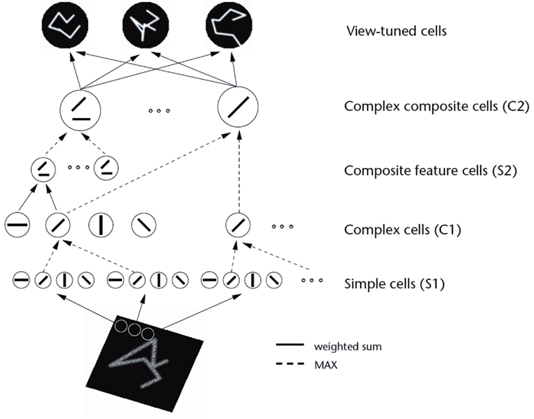
Figure 40. Sketch of Riesenhuber and Poggio’s (1999a,b) model of invariant object recognition. The model includes layers of “S” cells which perform template matching (solid lines), and “C” cells (solid lines) which pool information by a non-linear MAX function to achieve invariance (see text). (After Riesenhuber and Poggio, 1999a,b.)

The function of each S cell layer is to build more complicated features from the inputs, and works by template matching. The function of each “C” cell layer is to provide some translation invariance over the features discovered in the preceding simple cell layer (as in Fukushima, 1980), and operates by performing a MAX function on the inputs. The non-linear MAX function makes a complex cell respond only to whatever is the highest activity input being received, and is part of the process by which invariance is achieved according to this proposal. This C layer process involves “implicitly scanning over afferents of the same type differing in the parameter of the transformation to which responses should be invariant (for instance, feature size for scale invariance), and then selecting the best-matching afferent” (Riesenhuber and Poggio, 1999b). Brain mechanisms by which this computation could be set up are not part of the scheme, and the model does not incorporate learning in its architecture, so does not yet provide a biologically plausible model of invariant object recognition. The model receives as its inputs a set of symmetric spatial-frequency filters that are closely spaced in spatial-frequency, and maps these through pairs of convergence followed by MAX function layers, without learning. Whatever output appears in the final layer is then tested with a support vector machine to measure how well the output can be used by this very powerful subsequent learning stage to categorize different types of image. Whether that is a good test of invariance learning is a matter for discussion (Pinto et al., 2008; see Section 8). The approach taken in VisNet is that instead of using a benchmark test of image exemplars from which to learn categories (Serre et al., 2007a,b,c), instead VisNet is trained to generalize across transforms of objects that provide the training set. However, the fact that the model of Poggio, Riesenhuber, Serre and colleagues does use a hierarchical approach to object recognition does represent useful convergent thinking toward how invariant object recognition may be implemented in the brain. Similarly, the approach of training a five-layer network with a more artificial gradient ascent approach with a goal function that does however include forming relatively time invariant representations and decorrelating the responses of neurons within each layer (Wyss et al., 2006; both processes that have their counterpart in VisNet), also reflects convergent thinking.

Further evidence consistent with the approach developed in the investigations of VisNet described in this paper comes from psychophysical studies. Wallis and Bülthoff (1999) and Perry et al. (2006) describe psychophysical evidence for learning of view-invariant representations by experience, in that the learning can be shown in special circumstances to be affected by the temporal sequence in which different views of objects are seen.

Another related approach, from the machine learning area, is that of convolutional networks. Convolutional Networks are a biologically inspired trainable architecture that can learn invariant features. Each stage in a ConvNet is composed of a filter bank, some non-linearities, and feature pooling layers. With multiple stages, a ConvNet can learn multi-level hierarchies of features (LeCun et al., 2010). Non-linearities that include rectification and local contrast normalization are important in such systems (Jarrett et al., 2009; and are of course properties of VisNet). Applications have been developed to visual object recognition and vision navigation for off-road mobile robots. Ullman has considered the use of features in a hierarchy to help with processes such as segmentation and object recognition (Ullman, 2007).

Another approach to the implementation of invariant representations in the brain is the use of neurons with Sigma-Pi synapses. Sigma-Pi synapses effectively allow one input to a synapse to be multiplied or gated by a second input to the synapse (Rolls, 2008b). The multiplying input might gate the appropriate set of the other inputs to a synapse to produce the shift or scale change required. For example, the multiplying input could be a signal that varies with the shift required to compute translation invariance, effectively mapping the appropriate set of x_j inputs through to the output neurons depending on the shift required (Olshausen et al., 1993, 1995; Mel et al., 1998; Mel and Fiser, 2000). Local operations on a dendrite could be involved in such a process (Mel et al., 1998). The explicit neural implementation of the gating mechanism seems implausible, given the need to multiply and thus remap large parts of the retinal input depending on shift and scale modifying connections to a particular set of output neurons. Moreover, the explicit control signal to set the multiplication required in V1 has not been identified. Moreover, if this was the solution used by the brain, the whole problem of shift and scale invariance could in principle be solved in one-layer of the system, rather than with the multiple hierarchically organized set of layers actually used in the brain, as shown schematically in Figure 1. The multiple-layers actually used in the brain are much more consistent with the type of scheme incorporated in VisNet. Moreover, if a multiplying system of the type hypothesized by Olshausen et al. (1993), Mel et al. (1998), and Olshausen et al. (1995) was implemented in a multilayer hierarchy with the shift and scale change emerging gradually, then the multiplying control signal would need to be supplied to every stage of the hierarchy. A further problem with such approaches is how the system is trained in the first place.

8. Measuring the Capacity of VisNet

For a theory of the brain mechanisms of invariant object recognition, it is important that the system should scale up, so that if a model such as VisNet was the size of the human visual system, it would have comparable performance. Most of the research with VisNet to date has focused on the principles of operation of the system, and what aspects of invariant object recognition the model can solve (Rolls, 2008b). In this section I consider how the system performs in its scaled up version (VisNetL, with 128 × 128 neurons in each of 4 layers). I compare the capacity of VisNetL with that of another model, HMAX, as that has been described as competing with state of the art systems (Serre et al., 2007a,b,c; Mutch and Lowe, 2008), and I raise interesting issues about how to measure the capacity of systems for invariant object recognition in natural scenes.

The tests (performed by L. Robinson of the Department of Computer Science, University of Warwick, UK and E. T. Rolls) utilized a benchmark approach incorporated in the work of Serre, Mutch, Poggio and colleagues (Serre et al., 2007b,c; Mutch and Lowe, 2008) and indeed typical of many standard approaches in computer vision. This uses standard datasets such as the Caltech-256 (Griffin et al., 2007) in which sets of images from different categories are to be classified.

8.1. Object Benchmark Databases

The Caltech-256 dataset (Griffin et al., 2007) is comprised of 256 object classes made up of images that have many aspect ratios, sizes and differ quite significantly in quality (having being manually collated from web searches). The objects within the images show significant intra-class variation and have a variety of poses, illumination, scale, and occlusion as expected from natural images (see examples in Figure 41). In this sense, the Caltech-256 database is considered to be a difficult challenge to object recognition systems. I come to the conclusion below that the benchmarking approach with this type of dataset is not useful for training a system that must learn invariant object representations. The reason for this is that the exemplars of each category in the Caltech-256 dataset are too discontinuous to provide a basis for learning invariant object representations. For example, the exemplars within a category in these datasets may be very different indeed.

FIGURE 41

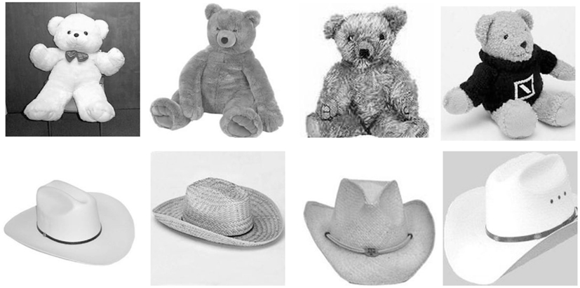
Figure 41. Example images from the Caltech-256 database for two object classes, teddy-bears and cowboy-hats.

Partly because of the limitations of the Caltech-256 database for training in invariant object recognition, we also investigated training with the Amsterdam Library of Images (ALOI; Geusebroek et al., 2005) database¹. The ALOI database takes a different approach to the Caltech-256, and instead of focusing on a set of natural images within a category, provides images with a systematic variation of pose and illumination for 1,000 small objects. Each object is placed onto a turntable and photographed in consistent conditions at 5° increments, resulting in a set of images that not only show the whole object (with regard to out of plane rotations), but does so with some continuity from one image to the next (see examples in Figure 42).

FIGURE 42

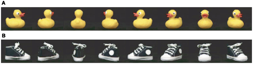
Figure 42. Example images from the two object classes within the ALOI database, (A) 90 (rubber duck) and (B) 93 (black shoe). Only the 45° increments are shown.

8.2. The HMAX Models Used for Comparison with VisNetL

The performance of VisNetL was compared against a standard HMAX model (Serre et al., 2007b,c; Mutch and Lowe, 2008), and a HMAX model scaled down to have a comparable complexity (in terms, for example, of the number of neurons) to that of VisNetL. The scaled down HMAX model is referred to as HMAX_min. The current HMAX family models have in the order of 10 million computational units (Serre et al., 2007b), which is at least 100 times the number contained within the current implementation of VisNetL (which uses 128 × 128 neurons in each of 4 layers, i.e., 65,536 neurons). In producing HMAX_min, we aimed to maintain the architectural features of HMAX, and primarily to scale it down. HMAX_min is based upon the “base” implementation of Mutch and Lowe (2008) ². The minimal version used in the comparisons differs from this base HMAX implementation in two significant ways. First, HMAX_min has only 4 scales compared to the 10 scales of HMAX. (Care was taken to ensure that HMAX_min still covered the same image size range – 256, 152, 90, and 53 pixels.) Second, the number of distinct units in the S2 “template matching” layer was limited to only 25 in HMAX_min, compared to 2,000 in HMAX. This results in a scaled down model HMAX_min, with approximately 12,000 units in the C1 layer, 75,000 units in the S2 layer, and 25 in the upper C2 layer, which is much closer to the 65,536 neurons of VisNetL. (The 75,000 units in S2 allow for every C2 neuron to be connected by its own weight to a C1 neuron.; When counting the number of neurons in the models, the number of neurons in S1 is not included, as they just provide the inputs to the models.)

8.3. Performance on a Caltech-256 Test

VisNetL and the two HMAX models were trained to discriminate between two object classes from the Caltech-256 database, the teddy-bear and cowboy-hat (see examples in Figure 41). Sixty image examples of each class were rescaled to 256 × 256 and converted to gray-scale, so that shape recognition was being investigated. The 60 images from each class were randomly partitioned into training and testing sets, with the training set size ranging over 1, 5, 15 and 30 images, and the corresponding testing set being the remainder of the 60 images in the cross-validation design. A linear support vector machine (libSVM, Chang and Lin, 2011) approach operating on the output of layer 4 of VisnetL was used to compare the categorization of the trained images with that of the test images, as that is the approach used by HMAX (Serre et al., 2007b,c; Mutch and Lowe, 2008). The standard default parameters of the support vector machine were used in identical form for the VisNetL and HMAX tests.

Figure 43 shows the performance of all three models when performing the task with the Caltech-256 dataset. It is clear that VisNetL performed better than HMAX_min as soon as there were reasonable numbers of training images, and this was confirmed statistically using the Chi-square test. It is also shown that the full HMAX model (as expected given its very large number of neurons) exhibits higher performance than that of VisNetL and HMAX_min.

FIGURE 43

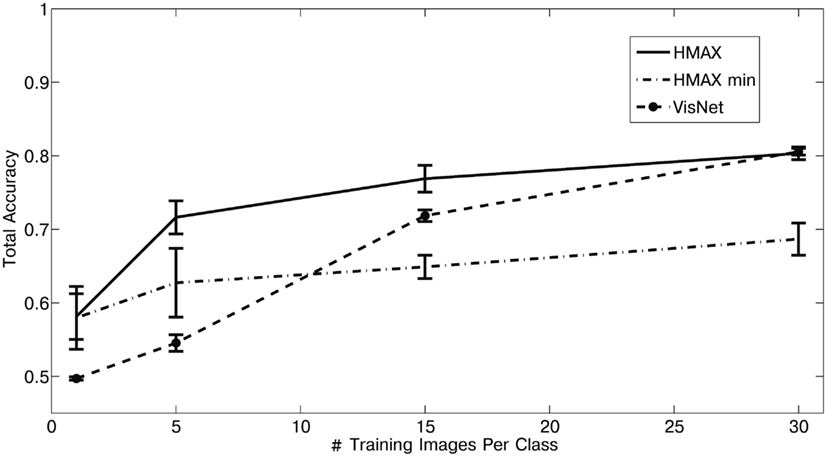
Figure 43. Performance of VisNetL, HMAX, and HMAX_min on the classification task using the Caltech-256 dataset. The error bars show the standard error of the means over 5 cross-validation trials with different images chosen at random for the training set on each trial. It is clear that VisNetL performs better than HMAX_min, and this was confirmed statistically using the Chi-square test performed with 30 training images and 30 cross-validation test images in each of two categories (Chi-square = 8.09, df = 1, p = 0.0025).

8.4. Performance with the Amsterdam Library of Images

Eight classes of object (with designations 36, 90, 93, 103, 138, 156, 203, 161) from the dataset were chosen (see Figure 42, for example). Each class comprises of 72 images taken at 5° increments through the full 360° out of plane rotation. Three sets of training images were used. (1) Three training images per class were taken at 315, 0, and 45°. (2) Eight training images encompassing the entire rotation of the object were taken in 45° increments. (3) Eighteen training images also encompassing the entire rotation of the object were taken in 20° increments. The testing set consisted for each object of the remaining orientations from the set of 72 that were not present in the particular training set. The aim of using the different training sets was to investigate how close in viewing angle the training images need to be; and also to investigate the effects of using different numbers of training images.

Figure 44 shows that VisNetL performed better than HMAX_min as soon as there were even a few training images, with HMAX as expected performing better. VisNetL performed almost as well as the very much larger HMAX as soon as there were reasonable numbers of training images.

FIGURE 44

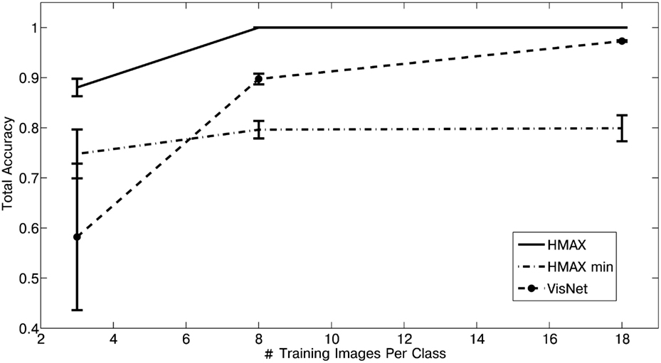
Figure 44. Performance of VisNetL, HMAX_min, and HMAX on the classification task with 8 classes using the Amsterdam Library of Images dataset. It is clear that VisNetL performs better than HMAX_min, and this was confirmed statistically using the Chi-square test performed with 18 training images 20° apart in view and 54 cross-validation testing images 5° apart in each of eight categories (Chi-square = 110.58, df = 1, p = 10⁻³).

What VisNetL can do here is to learn view-invariant representations using its trace-learning rule to build feature analyzers that reflect the similarity across at least adjacent views of the training set. Very interestingly, with 8 training images, the view spacing of the training images was 45°, and the test images in the cross-validation design were the intermediate views, 22.5° away from the nearest trained view. This is promising, for it shows that enormous numbers of training images with many different closely spaced views are not necessary for VisNetL. Even 8 training views spaced 45° apart produced reasonable training.

8.5. Individual Layer Performance

To test whether the VisNet hierarchy is actually performing useful computations with these datasets the simulations were re-run, though this time instead of only training the SVM on the activity generated in the final layer, four identical SVM’s were trained independently on the activities of each of the four layers. If the VisNet hierarchy is actually forming useful representations with these datasets then we should see the discriminatory power of SVMs trained on each layer increase as we traverse the hierarchy.

When the Caltech-256 dataset was used to train VisNetL there was very little difference in the measured performance of classifiers trained on each layer. This is revealing, for it shows that the Caltech-256 dataset does not have sufficient similarity between the exemplars within a given class for the trace-learning rule utilized in VisNet to perform useful learning. Thus, at least with a convergent feature hierarchy network trained in this way, there is insufficient similarity and information in the exemplars of each category of the Caltech-256 to learn to generalize in a view-invariant way to further exemplars of that category.

In contrast, when the ALOI dataset was used to train VisNetL the later layers performed better (layer 2–72% correct; layer 3–84% correct; layer 4–86% correct: p < 0.001). Thus there is sufficient continuity in the images in the ALOI dataset to support view-invariance learning in this feature hierarchy network.

8.6. Evaluation

One conclusion is that VisNetL performs comparably to a scaled down version of HMAX on benchmark tests. This is reassuring, for HMAX has been described as competing with state of the art systems (Serre et al., 2007a,b,c; Mutch and Lowe, 2008).

A second conclusion is that image databases such as the Caltech-256 that are used to test the performance of object recognition systems (Serre et al., 2007a,b,c; Mutch and Lowe, 2008; and in many computer vision approaches) are inappropriate as training sets for systems that perform invariant visual object recognition. Instead, for such systems, it will be much more relevant to train on image sets in which the image exemplars within a class show much more continuous variation. This provides the system with the opportunity to learn invariant representations, instead of just doing its best to categorize images into classes from relatively limited numbers of images that do not allow the system to learn the rules of the transforms that objects undergo in the real-world, and that can be used to help object recognition when objects may be seen from different views. This is an important conclusion for research in the area. Consistently, others are realizing that invariant visual object recognition is a hard problem (Pinto et al., 2008; DiCarlo et al., 2012). In this context, the hypotheses presented in this paper are my theory of how invariant visual object recognition is performed by the brain (Rolls, 1992, 2008b), and the model VisNet tests those hypotheses and provides a model for how invariant visual object representations can be learned (Rolls, 2008b).

Third, the findings described here are encouraging with respect to training view-invariant representations, in that the training images with the ALOI dataset could be separated by as much as 45° to still provide for view-invariant object recognition with cross-validation images that were never closer than 22.5° to a training image. This is helpful, for it is an indication that large numbers of different views will not need to be trained with the VisNet architecture in order to achieve good view-invariant object recognition.

9. Different Processes Involved in Different Types of Object Identification

To conclude this paper, it is proposed that there are (at least) three different types of process that could be involved in object identification. The first is the simple situation where different objects can be distinguished by different non-overlapping sets of features (see Section 3.1). An example might be a banana and an orange, where the list of features of the banana might include yellow, elongated, and smooth surface; and of the orange its orange color, round shape, and dimpled surface. Such objects could be distinguished just on the basis of a list of the properties, which could be processed appropriately by a competitive network, pattern associator, etc. No special mechanism is needed for view-invariance, because the list of properties is very similar from most viewing angles. Object recognition of this type may be common in animals, especially those with visual systems less developed than those of primates. However, this approach does not describe the shape and form of objects, and is insufficient to account for primate vision. Nevertheless, the features present in objects are valuable cues to object identity, and are naturally incorporated into the feature hierarchy approach.

A second type of process might involve the ability to generalize across a small range of views of an object, that is within a generic view, where cues of the first type cannot be used to solve the problem. An example might be generalization across a range of views of a cup when looking into the cup, from just above the near lip until the bottom inside of the cup comes into view. This type of process includes the learning of the transforms of the surface markings on 3D objects which occur when the object is rotated, as described in Section 5.6. Such generalization would work because the neurons are tuned as filters to accept a range of variation of the input within parameters such as relative size and orientation of the components of the features. Generalization of this type would not be expected to work when there is a catastrophic change in the features visible, as, for example, occurs when the cup is rotated so that one can suddenly no longer see inside it, and the outside bottom of the cup comes into view.

The third type of process is one that can deal with the sudden catastrophic change in the features visible when an object is rotated to a completely different view, as in the cup example just given (cf. Koenderink, 1990). Another example, quite extreme to illustrate the point, might be when a card with different images on its two sides is rotated so that one face and then the other is in view. This makes the point that this third type of process may involve arbitrary pairwise association learning, to learn which features and views are different aspects of the same object. Another example occurs when only some parts of an object are visible. For example, a red-handled screwdriver may be recognized either from its round red handle, or from its elongated silver-colored blade.

The full view-invariant recognition of objects that occurs even when the objects share the same features, such as color, texture, etc. is an especially computationally demanding task which the primate visual system is able to perform with its highly developed temporal lobe cortical visual areas. The neurophysiological evidence and the neuronal network analyses described here and elsewhere (Rolls, 2008b) provide clear hypotheses about how the primate visual system may perform this task.

10. Conclusion

We have seen that the feature hierarchy approach has a number of advantages in performing object recognition over other approaches (see Section 3), and that some of the key computational issues that arise in these architectures have solutions (see Sections 4 and 5). The neurophysiological and computational approach taken here focuses on a feature hierarchy model in which invariant representations can be built by self-organizing learning based on the statistics of the visual input.

The model can use temporal continuity in an associative synaptic learning rule with a short-term memory trace, and/or it can use spatial continuity in continuous spatial transformation learning.

The model of visual processing in the ventral cortical stream can build representations of objects that are invariant with respect to translation, view, size, and lighting.

The model uses a feature combination neuron approach with the relative spatial positions of the objects specified in the feature combination neurons, and this provides a solution to the binding problem.

The model has been extended to provide an account of invariant representations in the dorsal visual system of the global motion produced by objects such as looming, rotation, and object-based movement.

The model has been extended to incorporate top-down feedback connections to model the control of attention by biased competition in, for example, spatial and object search tasks (Deco and Rolls, 2004; Rolls, 2008b).

The model has also been extended to account for how the visual system can select single objects in complex visual scenes, how multiple objects can be represented in a scene, and how invariant representations of single objects can be learned even when multiple objects are present in the scene.

It has also been suggested in a unifying proposal that adding a fifth layer to the model and training the system in spatial environments will enable hippocampus-like spatial view neurons or place cells to develop, depending on the size of the field of view (Section 6).

We have thus seen how many of the major computational issues that arise when formulating a theory of object recognition in the ventral visual system (such as feature binding, invariance learning, the recognition of objects when they are in cluttered natural scenes, the representation of multiple objects in a scene, and learning invariant representations of single objects when there are multiple objects in the scene), could be solved in the brain, with tests of the hypotheses performed by simulations that are consistent with complementary neurophysiological results.

The approach described here is unifying in a number of ways. First, a set of simple organizational principles involving a hierarchy of cortical areas with convergence from stage to stage, and competitive learning using a modified associative learning rule with a short-term memory trace of preceding neuronal activity, provide a basis for understanding much processing in the ventral visual stream, from V1 to the inferior temporal visual cortex. Second, the same principles help to understand some of the processing in the dorsal visual stream by which invariant representations of the global motion of objects may be formed. Third, the same principles continued from the ventral visual stream onward to the hippocampus help to show how spatial view and place representations may be built from the visual input. Fourth, in all these cases, the learning is possible because the system is able to extract invariant representations because it can utilize the spatio-temporal continuities and statistics in the world that help to define objects, moving objects, and spatial scenes. Fifth, a great simplification and economy in terms of brain design is that the computational principles need not be different in each of the cortical areas in these hierarchical systems, for some of the important properties of the processing in these systems to be performed.

In conclusion, we have seen how the invariant recognition of objects involves not only the storage and retrieval of information, but also major computations to produce invariant representations. Once these invariant representations have been formed, they are used for many processes including not only recognition memory (Rolls, 2008b), but also associative learning of the rewarding and punishing properties of objects for emotion and motivation (Rolls, 2005, 2008b, 2013), the memory for the spatial locations of objects and rewards, the building of spatial representations based on visual input, and as an input to short-term memory, attention, decision, and action selection systems (Rolls, 2008b).

Conflict of Interest Statement

The author declares that the research was conducted in the absence of any commercial or financial relationships that could be construed as a potential conflict of interest.

Acknowledgments

Edmund T. Rolls is grateful to Larry Abbott, Nicholas Aggelopoulos, Roland Baddeley, Francesco Battaglia, Michael Booth, Gordon Baylis, Hugo Critchley, Gustavo Deco, Martin Elliffe, Leonardo Franco, Michael Hasselmo, Nestor Parga, David Perrett, Gavin Perry, Leigh Robinson, Simon Stringer, Martin Tovee, Alessandro Treves, James Tromans, and Tristan Webb for contributing to many of the collaborative studies described here. Professor R. Watt, of Stirling University, is thanked for assistance with the implementation of the difference of Gaussian filters used in many experiments with VisNet and VisNet2. Support from the Medical Research Council, the Wellcome Trust, the Oxford McDonnell Centre in Cognitive Neuroscience, and the Oxford Centre for Computational Neuroscience (www.oxcns.org, where .pdfs of papers are available) is acknowledged.

Footnotes

1. ^http://staff.science.uva.nl/aloi/
2. ^http://cbcl.mit.edu/jmutch/cns/index.html

References

Abbott, L. F., Rolls, E. T., and Tovee, M. J. (1996). Representational capacity of face coding in monkeys. Cereb. Cortex 6, 498–505.

Pubmed Abstract | Pubmed Full Text | CrossRef Full Text

Abeles, M. (1991). Corticonics: Neural Circuits of the Cerebral Cortex. Cambridge: Cambridge University Press.

Ackley, D. H., Hinton, G. E., and Sejnowski, T. J. (1985). A learning algorithm for Boltzmann machines. Cogn. Sci. 9, 147–169.

CrossRef Full Text

Aggelopoulos, N. C., Franco, L., and Rolls, E. T. (2005). Object perception in natural scenes: encoding by inferior temporal cortex simultaneously recorded neurons. J. Neurophysiol. 93, 1342–1357.

Pubmed Abstract | Pubmed Full Text | CrossRef Full Text

Aggelopoulos, N. C., and Rolls, E. T. (2005). Natural scene perception: inferior temporal cortex neurons encode the positions of different objects in the scene. Eur. J. Neurosci. 22, 2903–2916.

Pubmed Abstract | Pubmed Full Text | CrossRef Full Text

Amit, D. J. (1989). Modelling Brain Function. New York: Cambridge University Press.

Anzai, A., Peng, X., and Van Essen, D. C. (2007). Neurons in monkey visual area V2 encode combinations of orientations. Nat. Neurosci. 10, 1313–1321.

Pubmed Abstract | Pubmed Full Text | CrossRef Full Text

Arathorn, D. (2002). Map-Seeking Circuits in Visual Cognition: A Computational Mechanism for Biological and Machine Vision. Stanford, CA: Stanford University Press.

Arathorn, D. (2005). “Computation in the higher visual cortices: map-seeking circuit theory and application to machine vision,” in Proceedings of the AIPR 2004: 33rd Applied Imagery Pattern Recognition Workshop, 73–78.

Ballard, D. H. (1990). “Animate vision uses object-centred reference frames,” in Advanced Neural Computers, ed. R. Eckmiller (Elsevier: Amsterdam), 229–236.

Barlow, H. B. (1972). Single units and sensation: a neuron doctrine for perceptual psychology. Perception 1, 371–394.

Pubmed Abstract | Pubmed Full Text | CrossRef Full Text

Barlow, H. B. (1985). “Cerebral cortex as model builder,” in Models of the Visual Cortex, eds D. Rose and V. G. Dobson (Chichester: Wiley), 37–46.

Barlow, H. B., Kaushal, T. P., and Mitchison, G. J. (1989). Finding minimum entropy codes. Neural Comput. 1, 412–423.

CrossRef Full Text

Bartlett, M. S., and Sejnowski, T. J. (1997). “Viewpoint invariant face recognition using independent component analysis and attractor networks,” in Advances in Neural Information Processing Systems, Vol. 9, eds M. Mozer, M. Jordan, and T. Petsche (Cambridge, MA: MIT Press), 817–823.

Baylis, G. C., Rolls, E. T., and Leonard, C. M. (1985). Selectivity between faces in the responses of a population of neurons in the cortex in the superior temporal sulcus of the monkey. Brain Res. 342, 91–102.

Pubmed Abstract | Pubmed Full Text | CrossRef Full Text

Baylis, G. C., Rolls, E. T., and Leonard, C. M. (1987). Functional subdivisions of temporal lobe neocortex. J. Neurosci. 7, 330–342.

Pubmed Abstract | Pubmed Full Text

Bennett, A. (1990). Large competitive networks. Network 1, 449–462.

CrossRef Full Text

Biederman, I. (1972). Perceiving real-world scenes. Science 177, 77–80.

Pubmed Abstract | Pubmed Full Text | CrossRef Full Text

Biederman, I. (1987). Recognition-by-components: a theory of human image understanding. Psychol. Rev. 94, 115–147.

Pubmed Abstract | Pubmed Full Text | CrossRef Full Text

Binford, T. O. (1981). Inferring surfaces from images. Artif. Intell. 17, 205–244.

CrossRef Full Text

Blumberg, J., and Kreiman, G. (2010). How cortical neurons help us see: visual recognition in the human brain. J. Clin. Invest. 120, 3054–3063.

Pubmed Abstract | Pubmed Full Text | CrossRef Full Text

Bolles, R. C., and Cain, R. A. (1982). Recognizing and locating partially visible objects: the local-feature-focus method. Int. J. Robot. Res. 1, 57–82.

CrossRef Full Text

Booth, M. C. A., and Rolls, E. T. (1998). View-invariant representations of familiar objects by neurons in the inferior temporal visual cortex. Cereb. Cortex 8, 510–523.

Pubmed Abstract | Pubmed Full Text | CrossRef Full Text

Boussaoud, D., Desimone, R., and Ungerleider, L. G. (1991). Visual topography of area TEO in the macaque. J. Comp. Neurol. 306, 554–575.

Pubmed Abstract | Pubmed Full Text | CrossRef Full Text

Brady, M., Ponce, J., Yuille, A., and Asada, H. (1985). Describing surfaces, A. I. Memo 882. Artif. Intell. 17, 285–349.

Brincat, S. L., and Connor, C. E. (2006). Dynamic shape synthesis in posterior inferotemporal cortex. Neuron 49, 17–24.

Pubmed Abstract | Pubmed Full Text | CrossRef Full Text

Bruce, V. (1988). Recognising Faces. Hillsdale, NJ: Erlbaum.

Brun, V. H., Otnass, M. K., Molden, S., Steffenach, H. A., Witter, M. P., Moser, M. B., and Moser, E. I. (2002). Place cells and place recognition maintained by direct entorhinal–hippocampal circuitry. Science 296, 2243–2246.

Pubmed Abstract | Pubmed Full Text | CrossRef Full Text

Buckley, M. J., Booth, M. C. A., Rolls, E. T., and Gaffan, D. (2001). Selective perceptual impairments following perirhinal cortex ablation. J. Neurosci. 21, 9824–9836.

Pubmed Abstract | Pubmed Full Text

Buhmann, J., Lange, J., von der Malsburg, C., Vorbrüggen, J. C., and Würtz, R. P. (1991). “Object recognition in the dynamic link architecture: parallel implementation of a transputer network,” in Neural Networks for Signal Processing, ed. B. Kosko (Englewood Cliffs, NJ: Prentice-Hall), 121–159.

Carlson, E. T., Rasquinha, R. J., Zhang, K., and Connor, C. E. (2011). A sparse object coding scheme in area v4. Curr. Biol. 21, 288–293.

Pubmed Abstract | Pubmed Full Text | CrossRef Full Text

Cerella, J. (1986). Pigeons and perceptrons. Pattern Recognit. 19, 431–438.

CrossRef Full Text

Chakravarty, I. (1979). A generalized line and junction labeling scheme with applications to scene analysis. IEEE Trans. Pattern Anal. Mach. Intell. 1, 202–205.

Pubmed Abstract | Pubmed Full Text | CrossRef Full Text

Chang, C.-C., and Lin, C.-J. (2011). LIBSVM: a library for support vector machines. ACM Trans. Intell. Syst. Technol. 2, 27.

Dane, C., and Bajcsy, R. (1982). “An object-centred three-dimensional model builder,” in Proceedings of the 6th International Conference on Pattern Recognition, Munich, 348–350.

Daugman, J. (1988). Complete discrete 2D-Gabor transforms by neural networks for image analysis and compression. IEEE Trans. Acoust. 36, 1169–1179.

CrossRef Full Text

De Araujo, I. E. T., Rolls, E. T., and Stringer, S. M. (2001). A view model which accounts for the response properties of hippocampal primate spatial view cells and rat place cells. Hippocampus 11, 699–706.

Pubmed Abstract | Pubmed Full Text | CrossRef Full Text

De Valois, R. L., and De Valois, K. K. (1988). Spatial Vision. New York: Oxford University Press.

Deco, G., and Rolls, E. T. (2004). A neurodynamical cortical model of visual attention and invariant object recognition. Vision Res. 44, 621–644.

Pubmed Abstract | Pubmed Full Text | CrossRef Full Text

Deco, G., and Rolls, E. T. (2005a). Attention, short term memory, and action selection: a unifying theory. Prog. Neurobiol. 76, 236–256.

CrossRef Full Text

Deco, G., and Rolls, E. T. (2005b). Neurodynamics of biased competition and cooperation for attention: a model with spiking neurons. J. Neurophysiol. 94, 295–313.

CrossRef Full Text

Desimone, R., and Duncan, J. (1995). Neural mechanisms of selective visual attention. Annu. Rev. Neurosci. 18, 193–222.

Pubmed Abstract | Pubmed Full Text | CrossRef Full Text

DeWeese, M. R., and Meister, M. (1999). How to measure the information gained from one symbol. Network 10, 325–340.

Pubmed Abstract | Pubmed Full Text | CrossRef Full Text

DiCarlo, J. J., and Maunsell, J. H. R. (2003). Anterior inferotemporal neurons of monkeys engaged in object recognition can be highly sensitive to object retinal position. J. Neurophysiol. 89, 3264–3278.

Pubmed Abstract | Pubmed Full Text | CrossRef Full Text

DiCarlo, J. J., Zoccolan, D., and Rust, N. C. (2012). How does the brain solve visual object recognition? Neuron 73, 415–434.

Pubmed Abstract | Pubmed Full Text | CrossRef Full Text

Dolan, R. J., Fink, G. R., Rolls, E. T., Booth, M., Holmes, A., Frackowiak, R. S. J., and Friston, K. J. (1997). How the brain learns to see objects and faces in an impoverished context. Nature 389, 596–599.

Pubmed Abstract | Pubmed Full Text | CrossRef Full Text

Dow, B. W., Snyder, A. Z., Vautin, R. G., and Bauer, R. (1981). Magnification factor and receptive field size in foveal striate cortex of the monkey. Exp. Brain Res. 44, 213–218.

Pubmed Abstract | Pubmed Full Text | CrossRef Full Text

Edelman, S. (1999). Representation and Recognition in Vision. Cambridge, MA: MIT Press.

Elliffe, M. C. M., Rolls, E. T., Parga, N., and Renart, A. (2000). A recurrent model of transformation invariance by association. Neural Netw. 13, 225–237.

Pubmed Abstract | Pubmed Full Text | CrossRef Full Text

Elliffe, M. C. M., Rolls, E. T., and Stringer, S. M. (2002). Invariant recognition of feature combinations in the visual system. Biol. Cybern. 86, 59–71.

Pubmed Abstract | Pubmed Full Text | CrossRef Full Text

Engel, A. K., Konig, P., Kreiter, A. K., Schillen, T. B., and Singer, W. (1992). Temporal coding in the visual system: new vistas on integration in the nervous system. Trends Neurosci. 15, 218–226.

Pubmed Abstract | Pubmed Full Text | CrossRef Full Text

Farah, M. J. (2000). The Cognitive Neuroscience of Vision. Oxford: Blackwell.

Farah, M. J., Meyer, M. M., and McMullen, P. A. (1996). The living/nonliving dissociation is not an artifact: giving an a priori implausible hypothesis a strong test. Cogn. Neuropsychol. 13, 137–154.

CrossRef Full Text

Faugeras, O. D. (1993). The Representation, Recognition and Location of 3-D Objects. Cambridge, MA: MIT Press.

Faugeras, O. D., and Hebert, M. (1986). The representation, recognition and location of 3-D objects. Int. J. Robot. Res. 5, 27–52.

CrossRef Full Text

Feldman, J. A. (1985). Four frames suffice: a provisional model of vision and space. Behav. Brain Sci. 8, 265–289.

CrossRef Full Text

Fenske, M. J., Aminoff, E., Gronau, N., and Bar, M. (2006). Top-down facilitation of visual object recognition: object-based and context-based contributions. Prog. Brain Res. 155, 3–21.

Pubmed Abstract | Pubmed Full Text | CrossRef Full Text

Field, D. J. (1987). Relations between the statistics of natural images and the response properties of cortical cells. J. Opt. Soc. Am. A 4, 2379–2394.

Pubmed Abstract | Pubmed Full Text | CrossRef Full Text

Field, D. J. (1994). What is the goal of sensory coding? Neural Comput. 6, 559–601.

CrossRef Full Text

Finkel, L. H., and Edelman, G. M. (1987). “Population rules for synapses in networks,” in Synaptic Function, eds G. M. Edelman, W. E. Gall, and W. M. Cowan (New York: John Wiley & Sons), 711–757.

Földiák, P. (1991). Learning invariance from transformation sequences. Neural Comput. 3, 193–199.

CrossRef Full Text

Földiák, P. (1992). Models of Sensory Coding. Technical Report CUED/F–INFENG/TR 91. Department of Engineering, University of Cambridge, Cambridge.

Folstein, J. R., Gauthier, I., and Palmeri, T. J. (2010). Mere exposure alters category learning of novel objects. Front. Psychol. 1:40. doi:10.3389/fpsyg.2010.00040

CrossRef Full Text

Franco, L., Rolls, E. T., Aggelopoulos, N. C., and Jerez, J. M. (2007). Neuronal selectivity, population sparseness, and ergodicity in the inferior temporal visual cortex. Biol. Cybern. 96, 547–560.

Pubmed Abstract | Pubmed Full Text | CrossRef Full Text

Franco, L., Rolls, E. T., Aggelopoulos, N. C., and Treves, A. (2004). The use of decoding to analyze the contribution to the information of the correlations between the firing of simultaneously recorded neurons. Exp. Brain Res. 155, 370–384.

Pubmed Abstract | Pubmed Full Text | CrossRef Full Text

Franzius, M., Sprekeler, H., and Wiskott, L. (2007). Slowness and sparseness lead to place, head-direction, and spatial-view cells. PLoS Comput. Biol. 3, e166. doi:10.1371/journal.pcbi.0030166

CrossRef Full Text

Freedman, D. J., and Miller, E. K. (2008). Neural mechanisms of visual categorization: insights from neurophysiology. Neurosci. Biobehav. Rev. 32, 311–329.

Pubmed Abstract | Pubmed Full Text | CrossRef Full Text

Freiwald, W. A., Tsao, D. Y., and Livingstone, M. S. (2009). A face feature space in the macaque temporal lobe. Nat. Neurosci. 12, 1187–1196.

Pubmed Abstract | Pubmed Full Text | CrossRef Full Text

Frey, B. J., and Jojic, N. (2003). Transformation-invariant clustering using the EM algorithm. IEEE Trans. Pattern Anal. Mach. Intell. 25, 1–17.

CrossRef Full Text

Fries, P. (2005). A mechanism for cognitive dynamics: neuronal communication through neuronal coherence. Trends Cogn. Sci. (Regul. Ed.) 9, 474–480.

Pubmed Abstract | Pubmed Full Text | CrossRef Full Text

Fries, P. (2009). Neuronal gamma-band synchronization as a fundamental process in cortical computation. Annu. Rev. Neurosci. 32, 209–224.

Pubmed Abstract | Pubmed Full Text | CrossRef Full Text

Fukushima, K. (1975). Cognitron: a self-organizing neural network. Biol. Cybern. 20, 121–136.

Pubmed Abstract | Pubmed Full Text | CrossRef Full Text

Fukushima, K. (1980). Neocognitron: a self-organizing neural network model for a mechanism of pattern recognition unaffected by shift in position. Biol. Cybern. 36, 193–202.

Pubmed Abstract | Pubmed Full Text | CrossRef Full Text

Fukushima, K. (1988). Neocognitron: a hierarchical neural network model capable of visual pattern recognition unaffected by shift in position. Neural Netw. 1, 119–130.

CrossRef Full Text

Fukushima, K. (1989). Analysis of the process of visual pattern recognition by the neocognitron. Neural Netw. 2, 413–420.

CrossRef Full Text

Fukushima, K. (1991). Neural networks for visual pattern recognition. IEEE Trans. E 74, 179–190.

Fukushima, K., and Miyake, S. (1982). Neocognitron: a new algorithm for pattern recognition tolerant of deformations and shifts in position. Pattern Recognit. 15, 455–469.

CrossRef Full Text

Fyhn, M., Molden, S., Witter, M. P., Moser, E. I., and Moser, M.-B. (2004). Spatial representation in the entorhinal cortex. Science 2004, 1258–1264.

CrossRef Full Text

Gardner, E. (1988). The space of interactions in neural network models. J. Phys. A Math. Gen. 21, 257–270.

CrossRef Full Text

Garthwaite, J. (2008). Concepts of neural nitric oxide-mediated transmission. Eur. J. Neurosci. 27, 2783–3802.

Pubmed Abstract | Pubmed Full Text | CrossRef Full Text

Geesaman, B. J., and Andersen, R. A. (1996). The analysis of complex motion patterns by form/cue invariant MSTd neurons. J. Neurosci. 16, 4716–4732.

Pubmed Abstract | Pubmed Full Text

Georges-François, P., Rolls, E. T., and Robertson, R. G. (1999). Spatial view cells in the primate hippocampus: allocentric view not head direction or eye position or place. Cereb. Cortex 9, 197–212.

Pubmed Abstract | Pubmed Full Text | CrossRef Full Text

Geusebroek, J.-M., Burghouts, G. J., and Smeulders, A. W. M. (2005). The Amsterdam library of object images. Int. J. Comput. Vis. 61, 103–112.

CrossRef Full Text

Gibson, J. J. (1950). The Perception of the Visual World. Boston: Houghton Mifflin.

Gibson, J. J. (1979). The Ecological Approach to Visual Perception. Boston: Houghton Mifflin.

Grabenhorst, F., and Rolls, E. T. (2011). Value, pleasure, and choice systems in the ventral prefrontal cortex. Trends Cogn. Sci. (Regul. Ed.) 15, 56–67.

Pubmed Abstract | Pubmed Full Text | CrossRef Full Text

Graziano, M. S. A., Andersen, R. A., and Snowden, R. J. (1994). Tuning of MST neurons to spiral motions. J. Neurosci. 14, 54–67.

Pubmed Abstract | Pubmed Full Text

Griffin, G., Holub, A., and Perona, P. (2007). The Caltech-256. Caltech Technical Report, Los Angeles, 1–20.

Grimson, W. E. L. (1990). Object Recognition by Computer. Cambridge, MA: MIT Press.

Griniasty, M., Tsodyks, M. V., and Amit, D. J. (1993). Conversion of temporal correlations between stimuli to spatial correlations between attractors. Neural Comput. 35, 1–17.

CrossRef Full Text

Gross, C. G., Desimone, R., Albright, T. D., and Schwartz, E. L. (1985). Inferior temporal cortex and pattern recognition. Exp. Brain Res. 11(Suppl.), 179–201.

Hafting, T., Fyhn, M., Molden, S., Moser, M. B., and Moser, E. I. (2005). Microstructure of a spatial map in the entorhinal cortex. Nature 436, 801–806.

Pubmed Abstract | Pubmed Full Text | CrossRef Full Text

Hasselmo, M. E., Rolls, E. T., and Baylis, G. C. (1989a). The role of expression and identity in the face-selective responses of neurons in the temporal visual cortex of the monkey. Behav. Brain Res. 32, 203–218.

CrossRef Full Text

Hasselmo, M. E., Rolls, E. T., Baylis, G. C., and Nalwa, V. (1989b). Object-centered encoding by face-selective neurons in the cortex in the superior temporal sulcus of the monkey. Exp. Brain Res. 75, 417–429.

CrossRef Full Text

Hawken, M. J., and Parker, A. J. (1987). Spatial properties of the monkey striate cortex. Proc. R. Soc. Lond. B Biol. Sci. 231, 251–288.

Pubmed Abstract | Pubmed Full Text | CrossRef Full Text

Hegde, J., and Van Essen, D. C. (2000). Selectivity for complex shapes in primate visual area V2. J. Neurosci. 20, RC61.

Pubmed Abstract | Pubmed Full Text

Hegde, J., and Van Essen, D. C. (2003). Strategies of shape representation in macaque visual area V2. Vis. Neurosci. 20, 313–328.

Pubmed Abstract | Pubmed Full Text | CrossRef Full Text

Hegde, J., and Van Essen, D. C. (2007). A comparative study of shape representation in macaque visual areas V2 and V4. Cereb. Cortex 17, 1100–1116.

Pubmed Abstract | Pubmed Full Text | CrossRef Full Text

Herrnstein, R. J. (1984). “Objects, categories, and discriminative stimuli,” in Animal Cognition, Chap. 14, eds H. L. Roitblat, T. G. Bever, and H. S. Terrace (Hillsdale, NJ: Lawrence Erlbaum and Associates), 233–261.

Hertz, J. A., Krogh, A., and Palmer, R. G. (1991). Introduction to the Theory of Neural Computation. Wokingham: Addison-Wesley.

Hestrin, S., Sah, P., and Nicoll, R. (1990). Mechanisms generating the time course of dual component excitatory synaptic currents recorded in hippocampal slices. Neuron 5, 247–253.

Pubmed Abstract | Pubmed Full Text | CrossRef Full Text

Hinton, G. E. (2010). Learning to represent visual input. Philos. Trans. R. Soc. Lond. B Biol. Sci. 365, 177–184.

Pubmed Abstract | Pubmed Full Text | CrossRef Full Text

Hinton, G. E., Dayan, P., Frey, B. J., and Neal, R. M. (1995). The “wake-sleep” algorithm for unsupervised neural networks. Science 268, 1158–1161.

Pubmed Abstract | Pubmed Full Text | CrossRef Full Text

Hinton, G. E., and Ghahramani, Z. (1997). Generative models for discovering sparse distributed representations. Philos. Trans. R. Soc. Lond. B Biol. Sci. 352, 1177–1190.

Pubmed Abstract | Pubmed Full Text | CrossRef Full Text

Hinton, G. E., and Sejnowski, T. J. (1986). “Learning and relearning in Boltzmann machines,” in Parallel Distributed Processing, Vol. 1, Chap. 7, eds D. Rumelhart and J. L. McClelland (Cambridge, MA: MIT Press), 282–317.

Hopfield, J. J. (1982). Neural networks and physical systems with emergent collective computational abilities. Proc. Natl. Acad. Sci. U. S. A. 79, 2554–2558.

Pubmed Abstract | Pubmed Full Text | CrossRef Full Text

Hubel, D. H., and Wiesel, T. N. (1962). Receptive fields, binocular interaction, and functional architecture in the cat’s visual cortex. J. Physiol. 160, 106–154.

Pubmed Abstract | Pubmed Full Text

Hubel, D. H., and Wiesel, T. N. (1968). Receptive fields and functional architecture of monkey striate cortex. J. Physiol. 195, 215–243.

Pubmed Abstract | Pubmed Full Text

Hummel, J. E., and Biederman, I. (1992). Dynamic binding in a neural network for shape recognition. Psychol. Rev. 99, 480–517.

Pubmed Abstract | Pubmed Full Text | CrossRef Full Text

Huttenlocher, D. P., and Ullman, S. (1990). Recognizing solid objects by alignment with an image. Int. J. Comput. Vis. 5, 195–212.

CrossRef Full Text

Ito, M. (1984). The Cerebellum and Neural Control. New York: Raven Press.

Ito, M. (1989). Long-term depression. Annu. Rev. Neurosci. 12, 85–102.

Pubmed Abstract | Pubmed Full Text | CrossRef Full Text

Ito, M., and Komatsu, H. (2004). Representation of angles embedded within contour stimuli in area V2 of macaque monkeys. J. Neurosci. 24, 3313–3324.

Pubmed Abstract | Pubmed Full Text | CrossRef Full Text

Itti, L., and Koch, C. (2000). A saliency-based search mechanism for overt and covert shifts of visual attention. Vision Res. 40, 1489–1506.

Pubmed Abstract | Pubmed Full Text | CrossRef Full Text

Jarrett, K., Kavukcuoglu, K., Ranzato, M., and Lecun, Y. (2009). “What is the best multi-stage architecture for object recognition?” in 2009 IEEE 12th International Conference on Computer Vision (ICCV), 2146–2153.

Jiang, F., Dricot, L., Weber, J., Righi, G., Tarr, M. J., Goebel, R., and Rossion, B. (2011). Face categorization in visual scenes may start in a higher order area of the right fusiform gyrus: evidence from dynamic visual stimulation in neuroimaging. J. Neurophysiol. 106, 2720–2736.

Pubmed Abstract | Pubmed Full Text | CrossRef Full Text

Koch, C. (1999). Biophysics of Computation. Oxford: Oxford University Press.

Koenderink, J. J. (1990). Solid Shape. Cambridge, MA: MIT Press.

Koenderink, J. J., and Van Doorn, A. J. (1979). The internal representation of solid shape with respect to vision. Biol. Cybern. 32, 211–217.

Pubmed Abstract | Pubmed Full Text | CrossRef Full Text

Koenderink, J. J., and van Doorn, A. J. (1991). Affine structure from motion. J. Opt. Soc. Am. A 8, 377–385.

Pubmed Abstract | Pubmed Full Text | CrossRef Full Text

Kourtzi, Z., and Connor, C. E. (2011). Neural representations for object perception: structure, category, and adaptive coding. Annu. Rev. Neurosci. 34, 45–67.

Pubmed Abstract | Pubmed Full Text | CrossRef Full Text

Kriegeskorte, N., Mur, M., Ruff, D. A., Kiani, R., Bodurka, J., Esteky, H., Tanaka, K., and Bandettini, P. A. (2008). Matching categorical object representations in inferior temporal cortex of man and monkey. Neuron 60, 1126–1141.

Pubmed Abstract | Pubmed Full Text | CrossRef Full Text

Krieman, G., Koch, C., and Fried, I. (2000). Category-specific visual responses of single neurons in the human medial temporal lobe. Nat. Neurosci. 3, 946–953.

Pubmed Abstract | Pubmed Full Text | CrossRef Full Text

Land, M. F. (1999). Motion and vision: why animals move their eyes. J. Comp. Physiol. A 185, 341–352.

Pubmed Abstract | Pubmed Full Text | CrossRef Full Text

Land, M. F., and Collett, T. S. (1997). “A survey of active vision in invertebrates,” in From Living Eyes to Seeing Machines, eds M. V. Srinivasan and S. Venkatesh (Oxford: Oxford University Press), 16–36.

LeCun, Y., Kavukcuoglu, K., and Farabet, C. (2010). “Convolutional networks and applications in vision,” in 2010 IEEE International Symposium on Circuits and Systems, 253–256.

Lee, T. S. (1996). Image representation using 2D Gabor wavelets. IEEE Trans. Pattern Anal. Mach. Intell. 18, 959–971.

CrossRef Full Text

Leen, T. K. (1995). From data distributions to regularization in invariant learning. Neural Comput. 7, 974–981.

CrossRef Full Text

Leibo, J. Z., Mutch, J., Rosasco, L., Ullman, S., and Poggio, T. (2010). Learning Generic Invariances in Object Recognition: Translation and Scale. MIT-CSAIL-TR-2010-061, Cambridge.

Li, N., and DiCarlo, J. J. (2008). Unsupervised natural experience rapidly alters invariant object representation in visual cortex. Science 321, 1502–1507.

Pubmed Abstract | Pubmed Full Text | CrossRef Full Text

Li, S., Mayhew, S. D., and Kourtzi, Z. (2011). Learning shapes spatiotemporal brain patterns for flexible categorical decisions. Cereb. Cortex. doi: 10.1093/cercor/bhr309. [Epub ahead of print].

CrossRef Full Text

Liu, J., Harris, A., and Kanwisher, N. (2010). Perception of face parts and face configurations: an fMRI study. J. Cogn. Neurosci. 22, 203–211.

Pubmed Abstract | Pubmed Full Text | CrossRef Full Text

Logothetis, N. K., Pauls, J., Bulthoff, H. H., and Poggio, T. (1994). View-dependent object recognition by monkeys. Curr. Biol. 4, 401–414.

Pubmed Abstract | Pubmed Full Text | CrossRef Full Text

Logothetis, N. K., Pauls, J., and Poggio, T. (1995). Shape representation in the inferior temporal cortex of monkeys. Curr. Biol. 5, 552–563.

Pubmed Abstract | Pubmed Full Text | CrossRef Full Text

Logothetis, N. K., and Sheinberg, D. L. (1996). Visual object recognition. Annu. Rev. Neurosci. 19, 577–621.

Pubmed Abstract | Pubmed Full Text | CrossRef Full Text

Lowe, D. (1985). Perceptual Organization and Visual Recognition. Boston: Kluwer.

Marr, D. (1982). Vision. San Francisco: Freeman.

Marr, D., and Nishihara, H. K. (1978). Representation and recognition of the spatial organization of three dimensional structure. Proc. R. Soc. Lond. B Biol. Sci. 200, 269–294.

Pubmed Abstract | Pubmed Full Text | CrossRef Full Text

McNaughton, B. L., Barnes, C. A., and O’Keefe, J. (1983). The contributions of position, direction, and velocity to single unit activity in the hippocampus of freely-moving rats. Exp. Brain Res. 52, 41–49.

Pubmed Abstract | Pubmed Full Text | CrossRef Full Text

Mel, B. W. (1997). SEEMORE: combining color, shape, and texture histogramming in a neurally-inspired approach to visual object recognition. Neural Comput. 9, 777–804.

Pubmed Abstract | Pubmed Full Text | CrossRef Full Text

Mel, B. W., and Fiser, J. (2000). Minimizing binding errors using learned conjunctive features. Neural Comput. 12, 731–762.

Pubmed Abstract | Pubmed Full Text | CrossRef Full Text

Mel, B. W., Ruderman, D. L., and Archie, K. A. (1998). Translation-invariant orientation tuning in visual “complex” cells could derive from intradendritic computations. J. Neurosci. 18, 4325–4334.

Pubmed Abstract | Pubmed Full Text

Mikami, A., Nakamura, K., and Kubota, K. (1994). Neuronal responses to photographs in the superior temporal sulcus of the rhesus monkey. Behav. Brain Res. 60, 1–13.

Pubmed Abstract | Pubmed Full Text | CrossRef Full Text

Milner, P. (1974). A model for visual shape recognition. Psychol. Rev. 81, 521–535.

Pubmed Abstract | Pubmed Full Text | CrossRef Full Text

Miyashita, Y. (1988). Neuronal correlate of visual associative long-term memory in the primate temporal cortex. Nature 335, 817–820.

Pubmed Abstract | Pubmed Full Text | CrossRef Full Text

Miyashita, Y., and Chang, H. S. (1988). Neuronal correlate of pictorial short-term memory in the primate temporal cortex. Nature 331, 68–70.

Pubmed Abstract | Pubmed Full Text | CrossRef Full Text

Montague, P. R., Gally, J. A., and Edelman, G. M. (1991). Spatial signalling in the development and function of neural connections. Cereb. Cortex 1, 199–220.

Pubmed Abstract | Pubmed Full Text | CrossRef Full Text

Moser, E. I. (2004). Hippocampal place cells demand attention. Neuron 42, 183–185.

Pubmed Abstract | Pubmed Full Text | CrossRef Full Text

Moser, M. B., and Moser, E. I. (1998). Functional differentiation in the hippocampus. Hippocampus 8, 608–619.

Pubmed Abstract | Pubmed Full Text | CrossRef Full Text

Movshon, J. A., Adelson, E. H., Gizzi, M. S., and Newsome, W. T. (1985). “The analysis of moving visual patterns,” in Pattern Recognition Mechanisms, eds C. Chagas, R. Gattass, and C. G. Gross (New York: Springer-Verlag), 117–151.

Mozer, M. C. (1991). The Perception of Multiple Objects: A Connectionist Approach. Cambridge, MA: MIT Press.

Muller, R. U., Kubie, J. L., Bostock, E. M., Taube, J. S., and Quirk, G. J. (1991). “Spatial firing correlates of neurons in the hippocampal formation of freely moving rats,” in Brain and Space, ed. J. P. Paillard (Oxford: Oxford University Press), 296–333.

Mundy, J., and Zisserman, A. (1992). “Introduction – towards a new framework for vision,” in Geometric Invariance in Computer Vision, eds J. Mundy and A. Zisserman (Cambridge, MA: MIT Press), 1–39.

Mutch, J., and Lowe, D. G. (2008). Object class recognition and localization using sparse features with limited receptive fields. Int. J. Comput. Vis. 80, 45–57.

CrossRef Full Text

Newsome, W. T., Britten, K. H., and Movshon, J. A. (1989). Neuronal correlates of a perceptual decision. Nature 341, 52–54.

Pubmed Abstract | Pubmed Full Text | CrossRef Full Text

Oja, E. (1982). A simplified neuron model as a principal component analyzer. J. Math. Biol. 15, 267–273.

Pubmed Abstract | Pubmed Full Text | CrossRef Full Text

O’Keefe, J. (1984). “Spatial memory within and without the hippocampal system,” in Neurobiology of the Hippocampus, ed. W. Seifert (London: Academic Press), 375–403.

Olshausen, B. A., Anderson, C. H., and Van Essen, D. C. (1993). A neurobiological model of visual attention and invariant pattern recognition based on dynamic routing of information. J. Neurosci. 13, 4700–4719.

Pubmed Abstract | Pubmed Full Text

Olshausen, B. A., Anderson, C. H., and Van Essen, D. C. (1995). A multiscale dynamic routing circuit for forming size- and position-invariant object representations. J. Comput. Neurosci. 2, 45–62.

Pubmed Abstract | Pubmed Full Text | CrossRef Full Text

Orban, G. A. (2011). The extraction of 3D shape in the visual system of human and nonhuman primates. Annu. Rev. Neurosci. 34, 361–388.

Pubmed Abstract | Pubmed Full Text | CrossRef Full Text

O’Reilly, J., and Munakata, Y. (2000). Computational Explorations in Cognitive Neuroscience. Cambridge, MA: MIT Press.

Parga, N., and Rolls, E. T. (1998). Transform invariant recognition by association in a recurrent network. Neural Comput. 10, 1507–1525.

Pubmed Abstract | Pubmed Full Text | CrossRef Full Text

Peng, H. C., Sha, L. F., Gan, Q., and Wei, Y. (1998). Energy function for learning invariance in multilayer perceptron. Electron. Lett. 34, 292–294.

CrossRef Full Text

Perrett, D. I., and Oram, M. W. (1993). Neurophysiology of shape processing. Image Vis. Comput. 11, 317–333.

CrossRef Full Text

Perrett, D. I., Rolls, E. T., and Caan, W. (1982). Visual neurons responsive to faces in the monkey temporal cortex. Exp. Brain Res. 47, 329–342.

Pubmed Abstract | Pubmed Full Text | CrossRef Full Text

Perrett, D. I., Smith, P. A. J., Potter, D. D., Mistlin, A. J., Head, A. S., Milner, D., and Jeeves, M. A. (1985). Visual cells in temporal cortex sensitive to face view and gaze direction. Proc. R. Soc. Lond. B Biol. Sci. 223, 293–317.

Pubmed Abstract | Pubmed Full Text | CrossRef Full Text

Perry, G., Rolls, E. T., and Stringer, S. M. (2006). Spatial vs temporal continuity in view invariant visual object recognition learning. Vision Res. 46, 3994–4006.

Pubmed Abstract | Pubmed Full Text | CrossRef Full Text

Perry, G., Rolls, E. T., and Stringer, S. M. (2010). Continuous transformation learning of translation invariant representations. Exp. Brain Res. 204, 255–270.

Pubmed Abstract | Pubmed Full Text | CrossRef Full Text

Pinto, N., Cox, D. D., and DiCarlo, J. J. (2008). Why is real-world visual object recognition hard? PLoS Comput. Biol. 4, e27. doi:10.1371/journal.pcbi.0040027

Pubmed Abstract | Pubmed Full Text | CrossRef Full Text

Poggio, T., and Edelman, S. (1990). A network that learns to recognize three-dimensional objects. Nature 343, 263–266.

Pubmed Abstract | Pubmed Full Text | CrossRef Full Text

Pollen, D., and Ronner, S. (1981). Phase relationship between adjacent simple cells in the visual cortex. Science 212, 1409–1411.

Pubmed Abstract | Pubmed Full Text | CrossRef Full Text

Rao, R. P. N., and Ruderman, D. L. (1999). “Learning lie groups for invariant visual perception,” in Advances in Neural Information Processing Systems, Vol. 11, eds M. S. Kearns, S. A. Solla, and D. A. Cohn (Cambridge: MIT Press), 810–816.

Renart, A., Parga, N., and Rolls, E. T. (2000). “A recurrent model of the interaction between the prefrontal cortex and inferior temporal cortex in delay memory tasks,” in Advances in Neural Information Processing Systems, Vol. 12, eds S. Solla, T. Leen, and K.-R. Mueller (Cambridge, MA: MIT Press), 171–177.

Rhodes, P. (1992). The open time of the NMDA channel facilitates the self-organisation of invariant object responses in cortex. Soc. Neurosci. Abstr. 18, 740.

Riesenhuber, M., and Poggio, T. (1998). “Just one view: invariances in inferotemporal cell tuning,” in Advances in Neural Information Processing Systems, Vol. 10, eds M. I. Jordan, M. J. Kearns, and S. A. Solla (Cambridge, MA: MIT Press), 215–221.

Riesenhuber, M., and Poggio, T. (1999a). Are cortical models really bound by the “binding problem”? Neuron 24, 87–93.

CrossRef Full Text

Riesenhuber, M., and Poggio, T. (1999b). Hierarchical models of object recognition in cortex. Nat. Neurosci. 2, 1019–1025.

CrossRef Full Text

Riesenhuber, M., and Poggio, T. (2000). Models of object recognition. Nat. Neurosci. 3(Suppl.), 1199–1204.

Pubmed Abstract | Pubmed Full Text | CrossRef Full Text

Ringach, D. L. (2002). Spatial structure and symmetry of simple-cell receptive fields in macaque primary visual cortex. J. Neurophysiol. 88, 455–463.

Pubmed Abstract | Pubmed Full Text

Robertson, R. G., Rolls, E. T., and Georges-François, P. (1998). Spatial view cells in the primate hippocampus: effects of removal of view details. J. Neurophysiol. 79, 1145–1156.

Pubmed Abstract | Pubmed Full Text

Rolls, E. T. (1989a). “Functions of neuronal networks in the hippocampus and neocortex in memory,” in Neural Models of Plasticity: Experimental and Theoretical Approaches, Chap. 13, eds J. H. Byrne and W. O. Berry (San Diego, CA: Academic Press), 240–265.

Rolls, E. T. (1989b). “The representation and storage of information in neuronal networks in the primate cerebral cortex and hippocampus,” in The Computing Neuron, Chap. 8, eds R. Durbin, C. Miall, and G. Mitchison (Wokingham: Addison-Wesley), 125–159.

Rolls, E. T. (1992). Neurophysiological mechanisms underlying face processing within and beyond the temporal cortical visual areas. Philos. Trans. R. Soc. Lond. B Biol. Sci. 335, 11–21.

Pubmed Abstract | Pubmed Full Text | CrossRef Full Text

Rolls, E. T. (1994). Brain mechanisms for invariant visual recognition and learning. Behav. Processes 33, 113–138.

CrossRef Full Text

Rolls, E. T. (1995). Learning mechanisms in the temporal lobe visual cortex. Behav. Brain Res. 66, 177–185.

Pubmed Abstract | Pubmed Full Text | CrossRef Full Text

Rolls, E. T. (1999). The Brain and Emotion. Oxford: Oxford University Press.

Rolls, E. T. (2000). Functions of the primate temporal lobe cortical visual areas in invariant visual object and face recognition. Neuron 27, 205–218.

Pubmed Abstract | Pubmed Full Text | CrossRef Full Text

Rolls, E. T. (2003). Consciousness absent and present: a neurophysiological exploration. Prog. Brain Res. 144, 95–106.

CrossRef Full Text

Rolls, E. T. (2005). Emotion Explained. Oxford: Oxford University Press.

Rolls, E. T. (2006). “Consciousness absent and present: a neurophysiological exploration of masking,” in The First Half Second, Chap. 6, eds H. Ogmen, and B. G. Breitmeyer (Cambridge, MA: MIT Press), 89–108.

Rolls, E. T. (2007a). “Invariant representations of objects in natural scenes in the temporal cortex visual areas,” in Representation and Brain, Chap. 3, ed. S. Funahashi (Tokyo: Springer), 47–102.

Rolls, E. T. (2007b). The representation of information about faces in the temporal and frontal lobes of primates including humans. Neuropsychologia 45, 124–143.

CrossRef Full Text

Rolls, E. T. (2007c). Sensory processing in the brain related to the control of food intake. Proc. Nutr. Soc. 66, 96–112.

CrossRef Full Text

Rolls, E. T. (2008a). Face representations in different brain areas, and critical band masking. J. Neuropsychol. 2, 325–360.

CrossRef Full Text

Rolls, E. T. (2008b). Memory, Attention, and Decision-Making. A Unifying Computational Neuroscience Approach. Oxford: Oxford University Press.

Rolls, E. T. (2008c). Top-down control of visual perception: attention in natural vision. Perception 37, 333–354.

CrossRef Full Text

Rolls, E. T. (2011a). David Marr’s vision: floreat computational neuroscience. Brain 134, 913–916.

CrossRef Full Text

Rolls, E. T. (2011b). “Face neurons,” in The Oxford Handbook of Face Perception, Chap. 4, eds A. J. Calder, G. Rhodes, M. H. Johnson, and J. V. Haxby (Oxford: Oxford University Press), 51–75.

Rolls, E. T. (2012). Neuroculture: On the Implications of Brain Science. Oxford: Oxford University Press.

Rolls, E. T. (2013). Emotion and Decision-Making Explained. Oxford: Oxford University Press.

Rolls, E. T., Aggelopoulos, N. C., Franco, L., and Treves, A. (2004). Information encoding in the inferior temporal visual cortex: contributions of the firing rates and the correlations between the firing of neurons. Biol. Cybern. 90, 19–32.

Pubmed Abstract | Pubmed Full Text | CrossRef Full Text

Rolls, E. T., Aggelopoulos, N. C., and Zheng, F. (2003). The receptive fields of inferior temporal cortex neurons in natural scenes. J. Neurosci. 23, 339–348.

Pubmed Abstract | Pubmed Full Text

Rolls, E. T., and Baylis, G. C. (1986). Size and contrast have only small effects on the responses to faces of neurons in the cortex of the superior temporal sulcus of the monkey. Exp. Brain Res. 65, 38–48.

Pubmed Abstract | Pubmed Full Text | CrossRef Full Text

Rolls, E. T., Baylis, G. C., Hasselmo, M., and Nalwa, V. (1989). “The representation of information in the temporal lobe visual cortical areas of macaque monkeys,” in Seeing Contour and Colour, eds J. Kulikowski, C. Dickinson, and I. Murray (Oxford: Pergamon).

Rolls, E. T., Baylis, G. C., and Hasselmo, M. E. (1987). The responses of neurons in the cortex in the superior temporal sulcus of the monkey to band-pass spatial frequency filtered faces. Vision Res. 27, 311–326.

Pubmed Abstract | Pubmed Full Text | CrossRef Full Text

Rolls, E. T., Baylis, G. C., and Leonard, C. M. (1985). Role of low and high spatial frequencies in the face-selective responses of neurons in the cortex in the superior temporal sulcus. Vision Res. 25, 1021–1035.

Pubmed Abstract | Pubmed Full Text | CrossRef Full Text

Rolls, E. T., and Deco, G. (2002). Computational Neuroscience of Vision. Oxford: Oxford University Press.

Rolls, E. T., and Deco, G. (2006). Attention in natural scenes: neurophysiological and computational bases. Neural Netw. 19, 1383–1394.

Pubmed Abstract | Pubmed Full Text | CrossRef Full Text

Rolls, E. T., Franco, L., Aggelopoulos, N. C., and Jerez, J. M. (2006a). Information in the first spike, the order of spikes, and the number of spikes provided by neurons in the inferior temporal visual cortex. Vision Res. 46, 4193–4205.

CrossRef Full Text

Rolls, E. T., Stringer, S. M., and Elliot, T. (2006b). Entorhinal cortex grid cells can map to hippocampal place cells by competitive learning. Network 17, 447–465.

CrossRef Full Text

Rolls, E. T., Franco, L., and Stringer, S. M. (2005a). The perirhinal cortex and long-term familiarity memory. Q. J. Exp. Psychol. B. 58, 234–245.

CrossRef Full Text

Rolls, E. T., Xiang, J.-Z., and Franco, L. (2005b). Object, space and object-space representations in the primate hippocampus. J. Neurophysiol. 94, 833–844.

CrossRef Full Text

Rolls, E. T., and Grabenhorst, F. (2008). The orbitofrontal cortex and beyond: from affect to decision-making. Prog. Neurobiol. 86, 216–244.

Pubmed Abstract | Pubmed Full Text | CrossRef Full Text

Rolls, E. T., and Milward, T. (2000). A model of invariant object recognition in the visual system: learning rules, activation functions, lateral inhibition, and information-based performance measures. Neural Comput. 12, 2547–2572.

Pubmed Abstract | Pubmed Full Text | CrossRef Full Text

Rolls, E. T., Robertson, R. G., and Georges-François, P. (1997a). Spatial view cells in the primate hippocampus. Eur. J. Neurosci. 9, 1789–1794.

CrossRef Full Text

Rolls, E. T., Treves, A., and Tovee, M. J. (1997b). The representational capacity of the distributed encoding of information provided by populations of neurons in the primate temporal visual cortex. Exp. Brain Res. 114, 149–162.

CrossRef Full Text

Rolls, E. T., Treves, A., Tovee, M., and Panzeri, S. (1997c). Information in the neuronal representation of individual stimuli in the primate temporal visual cortex. J. Comput. Neurosci. 4, 309–333.

CrossRef Full Text

Rolls, E. T., and Stringer, S. M. (2000). On the design of neural networks in the brain by genetic evolution. Prog. Neurobiol. 61, 557–579.

Pubmed Abstract | Pubmed Full Text | CrossRef Full Text

Rolls, E. T., and Stringer, S. M. (2001). Invariant object recognition in the visual system with error correction and temporal difference learning. Network 12, 111–129.

Pubmed Abstract | Pubmed Full Text | CrossRef Full Text

Rolls, E. T., and Stringer, S. M. (2006). Invariant visual object recognition: a model, with lighting invariance. J. Physiol. Paris 100, 43–62.

Pubmed Abstract | Pubmed Full Text | CrossRef Full Text

Rolls, E. T., and Stringer, S. M. (2007). Invariant global motion recognition in the dorsal visual system: a unifying theory. Neural Comput. 19, 139–169.

Pubmed Abstract | Pubmed Full Text | CrossRef Full Text

Rolls, E. T., and Tovee, M. J. (1994). Processing speed in the cerebral cortex and the neurophysiology of visual masking. Proc. R. Soc. Lond. B Biol. Sci. 257, 9–15.

CrossRef Full Text

Rolls, E. T., and Tovee, M. J. (1995a). The responses of single neurons in the temporal visual cortical areas of the macaque when more than one stimulus is present in the visual field. Exp. Brain Res. 103, 409–420.

CrossRef Full Text

Rolls, E. T., and Tovee, M. J. (1995b). Sparseness of the neuronal representation of stimuli in the primate temporal visual cortex. J. Neurophysiol. 73, 713–726.

Rolls, E. T., Tovee, M. J., and Panzeri, S. (1999). The neurophysiology of backward visual masking: information analysis. J. Cogn. Neurosci. 11, 335–346.

CrossRef Full Text

Rolls, E. T., Tovee, M. J., Purcell, D. G., Stewart, A. L., and Azzopardi, P. (1994). The responses of neurons in the temporal cortex of primates, and face identification and detection. Exp. Brain Res. 101, 474–484.

CrossRef Full Text

Rolls, E. T., and Treves, A. (1998). Neural Networks and Brain Function. Oxford: Oxford University Press.

Rolls, E. T., and Treves, A. (2011). The neuronal encoding of information in the brain. Prog. Neurobiol. 95, 448–490.

Pubmed Abstract | Pubmed Full Text | CrossRef Full Text

Rolls, E. T., Treves, A., Robertson, R. G., Georges-François, P., and Panzeri, S. (1998). Information about spatial view in an ensemble of primate hippocampal cells. J. Neurophysiol. 79, 1797–1813.

Pubmed Abstract | Pubmed Full Text

Rolls, E. T., Tromans, J. M., and Stringer, S. M. (2008). Spatial scene representations formed by self-organizing learning in a hippocampal extension of the ventral visual system. Eur. J. Neurosci. 28, 2116–2127.

Pubmed Abstract | Pubmed Full Text | CrossRef Full Text

Rolls, E. T., Webb, T. J., and Deco, G. (2012). Communication before coherence. Eur. J. Neurosci. (in press).

Rolls, E. T., and Xiang, J.-Z. (2006). Spatial view cells in the primate hippocampus, and memory recall. Rev. Neurosci. 17, 175–200.

Pubmed Abstract | Pubmed Full Text | CrossRef Full Text

Rosenblatt, F. (1961). Principles of Neurodynamics: Perceptrons and the Theory of Brain Mechanisms. Washington, DC: Spartan.

Sakai, K., and Miyashita, Y. (1991). Neural organisation for the long-term memory of paired associates. Nature 354, 152–155.

Pubmed Abstract | Pubmed Full Text | CrossRef Full Text

Sato, T. (1989). Interactions of visual stimuli in the receptive fields of inferior temporal neurons in macaque. Exp. Brain Res. 77, 23–30.

Pubmed Abstract | Pubmed Full Text | CrossRef Full Text

Selfridge, O. G. (1959). “Pandemonium: a paradigm for learning,” in The Mechanization of Thought Processes, eds D. Blake and A. Uttley (London: H. M. Stationery Office), 511–529.

Serre, T., Kreiman, G., Kouh, M., Cadieu, C., Knoblich, U., and Poggio, T. (2007a). A quantitative theory of immediate visual recognition. Prog. Brain Res. 165, 33–56.

CrossRef Full Text

Serre, T., Oliva, A., and Poggio, T. (2007b). A feedforward architecture accounts for rapid categorization. Proc. Natl. Acad. Sci. U.S.A. 104, 6424–6429.

CrossRef Full Text

Serre, T., Wolf, L., Bileschi, S., Riesenhuber, M., and Poggio, T. (2007c). Robust object recognition with cortex-like mechanisms. IEEE Trans. Pattern Anal. Mach. Intell. 29, 411–426.

CrossRef Full Text

Shadlen, M. N., and Movshon, J. A. (1999). Synchrony unbound: a critical evaluation of the temporal binding hypothesis. Neuron 24, 67–77.

Pubmed Abstract | Pubmed Full Text | CrossRef Full Text

Shashua, A. (1995). Algebraic functions for recognition. IEEE Trans. Pattern Anal. Mach. Intell. 17, 779–789.

CrossRef Full Text

Shevelev, I. A., Novikova, R. V., Lazareva, N. A., Tikhomirov, A. S., and Sharaev, G. A. (1995). Sensitivity to cross-like figures in cat striate neurons. Neuroscience 69, 51–57.

Pubmed Abstract | Pubmed Full Text | CrossRef Full Text

Sillito, A. M., Grieve, K. L., Jones, H. E., Cudeiro, J., and Davis, J. (1995). Visual cortical mechanisms detecting focal orientation discontinuities. Nature 378, 492–496.

Pubmed Abstract | Pubmed Full Text | CrossRef Full Text

Singer, W. (1999). Neuronal synchrony: a versatile code for the definition of relations? Neuron 24, 49–65.

Pubmed Abstract | Pubmed Full Text | CrossRef Full Text

Singer, W., Gray, C., Engel, A., Konig, P., Artola, A., and Brocher, S. (1990). Formation of cortical cell assemblies. Cold Spring Harb. Symp. Quant. Biol. 55, 939–952.

Pubmed Abstract | Pubmed Full Text | CrossRef Full Text

Singer, W., and Gray, C. M. (1995). Visual feature integration and the temporal correlation hypothesis. Annu. Rev. Neurosci. 18, 555–586.

Pubmed Abstract | Pubmed Full Text | CrossRef Full Text

Spiridon, M., Fischl, B., and Kanwisher, N. (2006). Location and spatial profile of category-specific regions in human extrastriate cortex. Hum. Brain Mapp. 27, 77–89.

Pubmed Abstract | Pubmed Full Text | CrossRef Full Text

Spruston, N., Jonas, P., and Sakmann, B. (1995). Dendritic glutamate receptor channel in rat hippocampal CA3 and CA1 pyramidal neurons. J. Physiol. 482, 325–352.

Pubmed Abstract | Pubmed Full Text

Stan-Kiewicz, B., and Hummel, J. (1994). “Metricat: a representation for basic and subordinate-level classification,” in Proceedings of the 18th Annual Conference of the Cognitive Science Society, ed. G. W. Cottrell (San Diego: Erlbaum), 254–259.

Stringer, S. M., Perry, G., Rolls, E. T., and Proske, J. H. (2006). Learning invariant object recognition in the visual system with continuous transformations. Biol. Cybern. 94, 128–142.

Pubmed Abstract | Pubmed Full Text | CrossRef Full Text

Stringer, S. M., and Rolls, E. T. (2000). Position invariant recognition in the visual system with cluttered environments. Neural Netw. 13, 305–315.

Pubmed Abstract | Pubmed Full Text | CrossRef Full Text

Stringer, S. M., and Rolls, E. T. (2002). Invariant object recognition in the visual system with novel views of 3D objects. Neural Comput. 14, 2585–2596.

Pubmed Abstract | Pubmed Full Text | CrossRef Full Text

Stringer, S. M., and Rolls, E. T. (2008). Learning transform invariant object recognition in the visual system with multiple stimuli present during training. Neural Netw. 21, 888–903.

Pubmed Abstract | Pubmed Full Text | CrossRef Full Text

Stringer, S. M., Rolls, E. T., and Tromans, J. M. (2007). Invariant object recognition with trace learning and multiple stimuli present during training. Network 18, 161–187.

Pubmed Abstract | Pubmed Full Text | CrossRef Full Text

Sutherland, N. S. (1968). Outline of a theory of visual pattern recognition in animal and man. Proc. R. Soc. Lond., B, Biol. Sci. 171, 297–317.

Pubmed Abstract | Pubmed Full Text

Sutton, R. S. (1988). Learning to predict by the methods of temporal differences. Mach. Learn. 3, 9–44.

CrossRef Full Text

Sutton, R. S., and Barto, A. G. (1981). Towards a modern theory of adaptive networks: expectation and prediction. Psychol. Rev. 88, 135–170.

Pubmed Abstract | Pubmed Full Text | CrossRef Full Text

Sutton, R. S., and Barto, A. G. (1998). Reinforcement Learning. Cambridge, MA: MIT Press.

Tanaka, K. (1993). Neuronal mechanisms of object recognition. Science 262, 685–688.

Pubmed Abstract | Pubmed Full Text | CrossRef Full Text

Tanaka, K. (1996). Inferotemporal cortex and object vision. Annu. Rev. Neurosci. 19, 109–139.

Pubmed Abstract | Pubmed Full Text | CrossRef Full Text

Tanaka, K., Saito, C., Fukada, Y., and Moriya, M. (1990). “Integration of form, texture, and color information in the inferotemporal cortex of the macaque,” in Vision, Memory and the Temporal Lobe, Chap. 10, eds E. Iwai and M. Mishkin (New York: Elsevier), 101–109.

Tanaka, K., Saito, H., Fukada, Y., and Moriya, M. (1991). Coding visual images of objects in the inferotemporal cortex of the macaque monkey. J. Neurophysiol. 66, 170–189.

Pubmed Abstract | Pubmed Full Text

Tou, J. T., and Gonzalez, A. G. (1974). Pattern Recognition Principles. Reading, MA: Addison-Wesley.

Tovee, M. J., and Rolls, E. T. (1995). Information encoding in short firing rate epochs by single neurons in the primate temporal visual cortex. Vis. Cogn. 2, 35–58.

CrossRef Full Text

Tovee, M. J., Rolls, E. T., and Azzopardi, P. (1994). Translation invariance and the responses of neurons in the temporal visual cortical areas of primates. J. Neurophysiol. 72, 1049–1060.

Pubmed Abstract | Pubmed Full Text

Tovee, M. J., Rolls, E. T., and Ramachandran, V. S. (1996). Rapid visual learning in neurones of the primate temporal visual cortex. Neuroreport 7, 2757–2760.

Pubmed Abstract | Pubmed Full Text | CrossRef Full Text

Tovee, M. J., Rolls, E. T., Treves, A., and Bellis, R. P. (1993). Information encoding and the responses of single neurons in the primate temporal visual cortex. J. Neurophysiol. 70, 640–654.

Pubmed Abstract | Pubmed Full Text

Trappenberg, T. P., Rolls, E. T., and Stringer, S. M. (2002). “Effective size of receptive fields of inferior temporal visual cortex neurons in natural scenes,” in Advances in Neural Information Processing Systems, Vol. 14, eds T. G. Dietterich, S. Becker, and Z. Gharamani (Cambridge, MA: MIT Press), 293–300.

Treves, A., and Rolls, E. T. (1991). What determines the capacity of autoassociative memories in the brain? Network 2, 371–397.

CrossRef Full Text

Tromans, J. M., Harris, M., and Stringer, S. M. (2011). A computational model of the development of separate representations of facial identity and expression in the primate visual system. PLoS ONE 6, e25616. doi:10.1371/journal.pone.0025616

CrossRef Full Text

Tromans, J. M., Page, J. I., and Stringer, S. M. (2012). Learning separate visual representations of independently rotating objects. Network. PMID: 22364581. [Epub ahead of print].

Pubmed Abstract | Pubmed Full Text

Tsao, D. Y., Freiwald, W. A., Tootell, R. B., and Livingstone, M. S. (2006). A cortical region consisting entirely of face-selective cells. Science 311, 617–618.

Pubmed Abstract | Pubmed Full Text | CrossRef Full Text

Tsao, D. Y., and Livingstone, M. S. (2008). Mechanisms of face perception. Annu. Rev. Neurosci. 31, 411–437.

Pubmed Abstract | Pubmed Full Text | CrossRef Full Text

Tsodyks, M. V., and Feigel’man, M. V. (1988). The enhanced storage capacity in neural networks with low activity level. Europhys. Lett. 6, 101–105.

CrossRef Full Text

Ullman, S. (1996). High-Level Vision, Object Recognition and Visual Cognition. Cambridge, MA: Bradford/MIT Press.

Ullman, S. (2007). Object recognition and segmentation by a fragment-based hierarchy. Trends Cogn. Sci. (Regul. Ed.) 11, 58–64.

Pubmed Abstract | Pubmed Full Text | CrossRef Full Text

Van Essen, D., Anderson, C. H., and Felleman, D. J. (1992). Information processing in the primate visual system: an integrated systems perspective. Science 255, 419–423.

Pubmed Abstract | Pubmed Full Text | CrossRef Full Text

Vogels, R., and Biederman, I. (2002). Effects of illumination intensity and direction on object coding in macaque inferior temporal cortex. Cereb. Cortex 12, 756–766.

Pubmed Abstract | Pubmed Full Text | CrossRef Full Text

von der Malsburg, C. (1973). Self-organization of orientation-sensitive columns in the striate cortex. Kybernetik 14, 85–100.

Pubmed Abstract | Pubmed Full Text | CrossRef Full Text

von der Malsburg, C. (1990). “A neural architecture for the representation of scenes,” in Brain Organization and Memory: Cells, Systems and Circuits, Chap. 18, eds J. L. McGaugh, N. M. Weinburger, and G. Lynch (Oxford: Oxford University Press), 356–372.

Wallis, G., and Baddeley, R. (1997). Optimal unsupervised learning in invariant object recognition. Neural Comput. 9, 883–894.

Pubmed Abstract | Pubmed Full Text | CrossRef Full Text

Wallis, G., and Bülthoff, H. (1999). Learning to recognize objects. Trends Cogn. Sci. (Regul. Ed.) 3, 22–31.

Pubmed Abstract | Pubmed Full Text | CrossRef Full Text

Wallis, G., and Rolls, E. T. (1997). Invariant face and object recognition in the visual system. Prog. Neurobiol. 51, 167–194.

Pubmed Abstract | Pubmed Full Text | CrossRef Full Text

Wallis, G., Rolls, E. T., and Foldiak, P. (1993). Learning invariant responses to the natural transformations of objects. Proc. Int. Jt. Conf. Neural Netw. 2, 1087–1090.

Wasserman, E., Kirkpatrick-Steger, A., and Biederman, I. (1998). Effects of geon deletion, scrambling, and movement on picture identification in pigeons. J. Exp. Psychol. Anim. Behav. Process. 24, 34–46.

Pubmed Abstract | Pubmed Full Text | CrossRef Full Text

Watanabe, S., Lea, S. E. G., and Dittrich, W. H. (1993). “What can we learn from experiments on pigeon discrimination?” in Vision, Brain, and Behavior in Birds, eds H. P. Zeigler, and H.-J. Bischof (Cambridge, MA: MIT Press), 351–376.

Weiner, K. S., and Grill-Spector, K. (2011). Neural representations of faces and limbs neighbor in human high-level visual cortex: evidence for a new organization principle. Psychol. Res. PMID: 22139022. [Epub ahead of print].

Pubmed Abstract | Pubmed Full Text

Widrow, B., and Hoff, M. E. (1960). “Adaptive switching circuits,” in 1960 IRE WESCON Convention Record, Part 4 (New York: IRE), 96–104. [Reprinted in Anderson and Rosenfeld, 1988].

Widrow, B., and Stearns, S. D. (1985). Adaptive Signal Processing. Englewood Cliffs, NJ: Prentice-Hall.

Winston, P. H. (1975). “Learning structural descriptions from examples,” in The Psychology of Computer Vision, ed. P. H. Winston (New York: McGraw-Hill), 157–210.

Wiskott, L. (2003). Slow feature analysis: a theoretical analysis of optimal free responses. Neural Comput. 15, 2147–2177.

Pubmed Abstract | Pubmed Full Text | CrossRef Full Text

Wiskott, L., and Sejnowski, T. J. (2002). Slow feature analysis: unsupervised learning of invariances. Neural Comput. 14, 715–770.

Pubmed Abstract | Pubmed Full Text | CrossRef Full Text

Womelsdorf, T., Schoffelen, J. M., Oostenveld, R., Singer, W., Desimone, R., Engel, A. K., and Fries, P. (2007). Modulation of neuronal interactions through neuronal synchronization. Science 316, 1609–1612.

Pubmed Abstract | Pubmed Full Text | CrossRef Full Text

Wurtz, R. H., and Kandel, E. R. (2000a). “Central visual pathways,” in Principles of Neural Science, 4th Edn, Chap. 27, eds E. R. Kandel, J. H. Schwartz, and T. M. Jessell (New York: McGraw-Hill), 543–547.

Wurtz, R. H., and Kandel, E. R. (2000b). “Perception of motion depth and form,” in Principles of Neural Science, 4th Edn, Chap. 28, eds E. R. Kandel, J. H. Schwartz, and T. M. Jessell (New York: McGraw-Hill), 548–571.

Wyss, R., Konig, P., and Verschure, P. F. (2006). A model of the ventral visual system based on temporal stability and local memory. PLoS Biol. 4, e120. doi:10.1371/journal.pbio.0040120

CrossRef Full Text

Yamane, S., Kaji, S., and Kawano, K. (1988). What facial features activate face neurons in the inferotemporal cortex of the monkey? Exp. Brain Res. 73, 209–214.

Pubmed Abstract | Pubmed Full Text | CrossRef Full Text

Yamane, Y., Carlson, E. T., Bowman, K. C., Wang, Z., and Connor, C. E. (2008). A neural code for three-dimensional object shape in macaque inferotemporal cortex. Nat. Neurosci. 11, 1352–1360.

Pubmed Abstract | Pubmed Full Text | CrossRef Full Text

Yi, D. J., Turk-Browne, N. B., Flombaum, J. I., Kim, M. S., Scholl, B. J., and Chun, M. M. (2008). Spatiotemporal object continuity in human ventral visual cortex. Proc. Natl. Acad. Sci. U.S.A. 105, 8840–8845.

Pubmed Abstract | Pubmed Full Text | CrossRef Full Text

Zhao, Q., and Koch, C. (2011). Learning a saliency map using fixated locations in natural scenes. J. Vis. 11, 9.

Pubmed Abstract | Pubmed Full Text | CrossRef Full Text

Zucker, S. W., Dobbins, A., and Iverson, L. (1989). Two stages of curve detection suggest two styles of visual computation. Neural Comput. 1, 68–81.

CrossRef Full Text