A generative spike train model with time-structured higher order correlations

1. Introduction

Recordings across the brain suggest that neural populations spike collectively—the statistics of their activity as a group are distinct from that expected in assembling the spikes from one cell at a time (Bair et al., 2001; Salinas and Sejnowski, 2001; Harris, 2005; Averbeck et al., 2006; Schneidman et al., 2006; Shlens et al., 2006; Pillow et al., 2008; Ganmor et al., 2011; Bathellier et al., 2012; Hansen et al., 2012; Luczak et al., 2013). Advances in electrode and imaging technology allow us to explore the dynamics of neural populations by simultaneously recording the activity of hundreds of cells. This is revealing patterns of collective spiking that extend across multiple cells. The underlying structure is intriguing: For example, higher-order interactions among cell groups have been observed widely (Amari et al., 2003; Schneidman et al., 2006; Shlens et al., 2006, 2009; Ohiorhenuan et al., 2010; Ganmor et al., 2011; Vasquez et al., 2012; Luczak et al., 2013). A number of recent studies point to mechanisms that generate such higher-order correlations from common input processes, including unobserved neurons. This suggests that, in a given recording or given set of neurons projecting downstream, higher-order correlations may be quite ubiquitous (Barreiro et al., 2010; Macke et al., 2011; Yu et al., 2011; Köster et al., 2013). Moreover, these higher-order correlations may impact the firing statistics of downstream neurons (Kuhn et al., 2003), the information capacity of their output (Ganmor et al., 2011; Cain and Shea-Brown, 2013; Montani et al., 2013), and could be essential in learning through spike-time dependent synaptic plasticity (Pfister and Gerstner, 2006; Gjorgjieva et al., 2011).

What exactly is the impact of such collective spiking on the encoding and transmission of information in the brain? This question has been studied extensively, but much remains unknown. Results to date show that the answers will be varied and rich. Patterned spiking can impact responses at the level of single cells (Salinas and Sejnowski, 2001; Kuhn et al., 2003; Xu et al., 2012) and neural populations (Amjad et al., 1997; Tetzlaff et al., 2003; Rosenbaum et al., 2010, 2011). Neurons with even the simplest of non-linearities can be highly sensitive to correlations in their inputs. Moreover, such non-linearities are sufficient to accurately decode signals from the input to correlated neural populations (Shamir and Sompolinsky, 2004).

An essential tool in understanding the impact of collective spiking is the ability to generate artificial spike trains with a predetermined structure across cells and across time (Brette, 2009; Gutnisky and Josić, 2009; Krumin and Shoham, 2009; Macke et al., 2009). Such synthetic spike trains are the grist for testing hypotheses about spatiotemporal patterns in coding and dynamics. In experimental studies, such spike trains can be used to provide structured stimulation of single cells across their dendritic trees via glutamate uncaging (Gasparini and Magee, 2006; Reddy et al., 2008; Branco et al., 2010; Branco and Häusser, 2011). In addition, entire populations of neurons can be activated via optical stimulation of microbial opsins (Han and Boyden, 2007; Chow et al., 2010). Computationally, they are used to examine the response of non-linear models of downstream cells (Carr et al., 1998; Salinas and Sejnowski, 2001; Kuhn et al., 2003).

Therefore, much effort has been devoted to developing statistical models of population activity. A number of flexible, yet tractable probabilistic models of joint neuronal activity have been proposed. Pairwise correlations are the most common type of interactions obtained from multi-unit recordings. Therefore, many earlier models were designed to generate samples of neural activity patterns with predetermined first and second order statistics (Brette, 2009; Gutnisky and Josić, 2009; Krumin and Shoham, 2009; Macke et al., 2009). In these models, higher-order correlations are not explicitly and separately controlled.

A number of different models have been used to analyze higher-order interactions. However, most of these models assume that interactions between different cells are instantaneous (or near-instantaneous) (Kuhn et al., 2003; Johnson and Goodman, 2009; Staude et al., 2010; Shimazaki et al., 2012). A notable exception is the work of Bäuerle and Grübel (2005), which developed such methods for use in financial applications. In these previous efforts, correlations at all orders were characterized by the increase, or decrease, in the probability that groups of cells spike together at the same time, or have a common temporal correlation structure regardless of the group.

The aim of the present work is to provide a statistical method for generating spike trains with more general correlation structures across cells and time. Specifically, we allow distinct temporal structure for correlations at pairwise, triplet, and all higher orders, and do so separately for different groups of cells in the neural population. Our aim to describe a model that can be applied in neuroscience, and can potentially be fit to emerging datasets.

A sample realization of a multivariate generalized thinning and shift (GTaS) process is shown in Figure 1. The multivariate spike train consists of six marginally Poisson processes. Each event was either uncorrelated with all other events across the population, or correlated in time with an event in all other spike trains. This model was configured to exhibit activity that cascades through a sequence of neurons. Specifically, neurons with larger index tend to fire later in a population wide event (this is similar to a synfire chain (Abeles, 1991), but with variable timing of spikes within the cascade). In Figure 1B, we plot the “population cross-cumulant density” for three chosen neurons—the summed activity of the population triggered by a spike in a chosen cell. The center of mass of this function measures the average latency by which spikes of the neuron in question precede those of the rest of the population (Luczak et al., 2013). Finally, Figure 1C shows the third-order cross-cumulant density for the three neurons. The triangular support of this function is a reflection of a synfire-like cascade structure of the spiking shown in the raster plot of panel (A): when firing events are correlated between trains, they tend to proceed in order of increasing index. We demonstrate the impact of such structured activity on a downstream network in section 2.2.3.

FIGURE 1

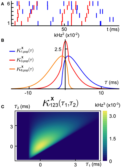
Figure 1. (A) Raster plot of event times for an example multivariate Poisson process X = (X₁, …, X₆) generated using the methods presented below. This model exhibits independent marginal events (blue) and population-level, chain-like events (red). (B) Some second order population cumulant densities (i.e., second order correlation between individual unit activities and population activity) for this model (Luczak et al., 2013). Greater mass to the right (resp. left) of τ = 0 indicates that the cell tends to lead (resp. follow) in pairwise-correlated events. (C) Third-order cross-cumulant density for processes X₁, X₂, X₃. The quantity κ^X₁₂₃(τ₁, τ₂) yields the probability of observing spikes in cells 2 and 3 at an offset τ₁, τ₂ from a spike in cell 1, respectively, in excess of what would be predicted from the first and second order cumulant structure. All quantities are precisely defined in the Methods. Note: system parameters necessary to reproduce results are given in the Appendix for all figures.

2. Results

Our aim is to describe a flexible multivariate point process capable of generating a range of high order correlation structures. To do so, we extend the TaS (thinning and shift) model of temporally- and spatially-correlated, marginally Poisson counting processes (Bäuerle and Grübel, 2005). The TaS model itself generalizes the SIP and MIP models (Kuhn et al., 2003) which have been used in theoretical neuroscience (Tetzlaff et al., 2008; Rosenbaum et al., 2010; Cain and Shea-Brown, 2013). However, the TaS model has not been used as widely. The original TaS model is too rigid to generate a number of interesting activity patterns observed in multi-unit recordings (Ikegaya et al., 2004; Luczak et al., 2007, 2013). We therefore developed the GTaS which allows for a more diverse temporal correlation structure.

We begin by describing the algorithm for sampling from the GTaS model. This constructive approach provides an intuitive understanding of the model's properties. We then present a pair of examples, the first of which highlights the utility of the GTaS framework. The second example demonstrates how sample point processes from the GTaS model can be used to study population dynamics. Next, we present the analysis which yields the explicit forms for the cross-cumulant densities derived in the context of the examples. We do so by first establishing a useful distributional representation for the GTaS process, paralleling Bäuerle and Grübel (2005). Using this representation, we derive cross-cumulants of a GTaS counting process, as well as explicit expressions for the cross-cumulant densities. After explaining the derivation at lower orders, we present a theorem which describes cross-cumulant densities at all orders.

2.1. GTaS Model Simulation

The GTaS model is parameterized first by a rate λ which determines the intensity of a “mother process”—a Poisson process on ℝ. The events of the mother process are marked, and the markings determine how each event is distributed among a collection of N daughter processes. The daughter processes are indexed by the set 𝔻 = {1, …, N}, and the set of possible markings is the power set 2^𝔻, the set of all subsets of 𝔻. We define a probability distribution p = (p_D)_{D ⊂ 𝔻}, assigning a probability to each possible marking, D. As we will see, p_D determines the probability of a joint event in all daughter processes with indices in the set D. Finally, to each marking, D, we assign a probability distribution Q_D, giving a family of shift (jitter) distributions (Q_D)_{D ⊂ 𝔻}. Each (Q_D) is a distribution over ℝ^N.

The rate λ, the distribution p over the markings, and the family of jitter distributions (Q_D)_{D ⊂ 𝔻}, define a vector X = (X₁, …, X_N) of dependent daughter Poisson processes described by the following algorithm, which yields a single realization (see Figure 2):

1. Simulate the mother Poisson process of rate λ on ℝ, generating a sequence of event times {t^j}. (Figure 2A).

2. With probability p_D^j assign the subset D^j ⊂ 𝔻 to the event of the mother process at time t^j. This event will be assigned only to processes with indices in D^j. (Figure 2B).

3. Sample a vector (Y^j₁, …, Y^j_N) = Y^j from the distribution Q_D^j. For each i ∈ D, the time t^j + Y^j_i is set as an event time for the marginal counting process X_i. (Figure 2C).

Hence copies of each point of the mother process are placed into daughter processes after a shift in time. A primary difference between the GTaS model and the TaS model presented in Bäuerle and Grübel (2005) is the dependence of the shift distributions Q_D on the chosen marking. This allows for greater flexibility in setting the temporal cumulant structure.

FIGURE 2

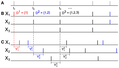
Figure 2. An illustration of a GTaS simulation. (A) Step 1: Simulate the mother process—a time-homogeneous Poisson process with event times {t^j}. (B) Step 2: For each t^j in step 1, select a set D^j ⊂ 𝔻 according to the distribution p_D, and project the event at time t^j to the subsets with indices in D^j. The legend indicates the colors assigned to three possible markings in this example. (C) Step 3: For each pair (t^j, D^j) generated in the previous two steps, draw Y^j from Q_D^j, and shift the event times in the daughter processes by the corresponding values Y^j_i.

2.2. Examples

2.2.1. Relation to SIP/MIP processes

Two simple models of correlated, jointly Poisson processes were defined in Kuhn et al. (2003). The resulting spike trains exhibit spatial correlations, but only instantaneous temporal dependencies. Each model was constructed by starting with independent Poisson processes, and applying one of two elementary point process operations: superposition and thinning (Cox and Isham, 1980). We show that both models are special cases of the GTaS model.

In the single interaction process (SIP), each marginal process X_i is obtained by merging an independent Poisson process with a common, global Poisson process. That is,

$X_i(·)=Z_i(·)+Z_c(·),i=1,\dots ,N,$

where Z_c and each Z_i are independent Poisson counting processes on ℝ with rates λ_c,λ_i, respectively. An SIP model is equivalent to a GTaS model with mother process rate λ = λ_c + ∑^N_{i = 1} λ_i, and marking probabilities

$p_D=\{\begin{array}{ll}\frac{{\lambda }_i}{\lambda }\hfill & D=\left\{i\right\}\hfill \\ \frac{{\lambda }_c}{\lambda }\hfill & D=𝔻\hfill \\ 0\hfill & \text{otherwise}\hfill \end{array}.$

Note that if λ_c = 0, each spike will be assigned to a different process X_i, resulting in N independent Poisson processes. Lastly, each shift distribution is equal to a delta distribution at zero in every coordinate (i.e., q_D(y₁, …, y_N) ≡ ∏^N_{i = 1}δ(y_i) for every D ⊂ 𝔻). Thus, all joint cumulants (among distinct marginal processes) of orders 2 through N are delta functions of equal magnitude, λp_𝔻.

The multiple interaction process (MIP) consists of N Poisson processes obtained from a common mother process with rate λ_m by thinning (Cox and Isham, 1980). The ith daughter process is formed by independent (across coordinates and events) deletion of events from the mother process with probability p = (1 − ϵ). Hence, an event is common to k daughter processes with probability ϵ^k. Therefore, if we take the perspective of retaining, rather than deleting events, the MIP model is equivalent to a GTaS process with λ = λ_m, and p_D = ϵ^|D|(1 − ϵ)^{d − |D|}. As in the SIP case, the shift distributions are singular in every coordinate. Below, we present a general result (Theorem 1.1) which immediately yields as a corollary that the MIP model has cross-cumulant functions which are δ functions in all dimensions, scaled by ϵ^k, where k is the order of the cross-cumulant.

2.2.2. Generation of synfire-like cascade activity

The GTaS framework provides a simple, tractable way of generating cascading activity where cells fire in a preferred order across the population—as in a synfire chain, but (in general) with variable timing of spikes (Abeles, 1991; Abeles and Prut, 1996; Aertsen et al., 1996; Aviel et al., 2002; Ikegaya et al., 2004). More generally, it can be used to simulate the activity of cell assemblies (Hebb, 1949; Harris, 2005; Buzsáki, 2010; Bathellier et al., 2012), in which the firing of groups of neurons is likely to follow a particular order.

In the Introduction, we briefly presented one example in which the GTaS framework was used to generate synfire-like cascade activity (see Figure 1), and we present another in Figure 3. In what follows, we will present the explicit definition of this second model, and then derive explicit expressions for its cumulant structure. Our aim is to illustrate the diverse range of possible correlation structures that can be generated using the GTaS model.

FIGURE 3

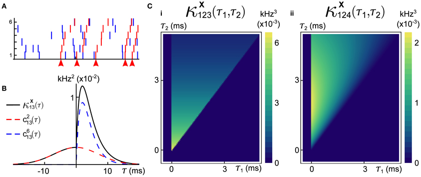
Figure 3. An example of a six dimensional GTaS model exhibiting synfire-like cascading firing patterns. (A) A raster-plot of spiking activity over a 100 ms window. Blue spikes indicate either marginal or pairwise events (i.e., events corresponding to markings for sets D ⊂𝔻 with |D| ≤ 2). Red spikes indicate population-wide events which have shift-times given by cumulative sums of independent exponentials, as described in the text. Arrows indicate the location of the first spike in the cascade. (B) A second-order cross-cumulant κ^X₁₃ (black line) of this model is composed of contributions from two sources: correlations due to second-order markings, which have Gaussian shifts (c²₁₃—dashed red line), and correlations due to the occurrence of population wide events (c^N₁₃—dashed blue line). (C) Density plots of the third-order cross-cumulant density for triplets (i) (1, 2, 3) and (ii) (1, 2, 4)—the latter is given explicitly in Equation (6). System parameters are given in the Appendix.

Consider an N-dimensional counting process X = (X₁, …, X_N) of GTaS type, where N ≥ 4. We restrict the marking distribution so that p_D ≡ 0 unless |D| ≤ 2 or D = 𝔻. That is, events are either assigned to a single, a pair, or all daughter processes. For sets D with |D| = 2, we set —a Gaussian distributions of zero mean and some specified covariance. The choice of the precise pairwise shift distributions is not important. Shifts of events attributed to a single process have no effect on the statistics of the multivariate process—this will become clear in section 2.3, when we exhibit that a GTaS process is equivalent in distribution to a sum of independent Poisson processes. In that context, the shifts of marginal events are applied to the event times of only one of these Poisson processes, which does not impact its statistics.

It remains to define the jitter distribution for events common to the entire population of daughter processes, i.e., events marked by 𝔻. We will show that we can generate cascading activity, and analytically describe the resulting correlation structure. We will say that a random variable T follows the exponential distribution Exp(α) if it has probability density

$f(t|\alpha )=\alpha e^{-\alpha t}\Theta (t),$

where Θ(t) is the Heaviside step function. We generate random vectors Y ~ Q_𝔻 according to the following rule, for each i = 1, …, N:

1. Generate independent random variables T_i ~ Exp(α_i) where α_i > 0.
2. Set Y_i = ∑ⁱ_{j = 1} T_j.

In particular, note that these shift times satisfy Y_N ≥… ≥ Y₂ ≥ Y₁ ≥ 0, indicating the chain-like structure of these joint events.

From the definition of the model and our general result (Theorem 1.1) below, we immediately have that κ^X_ij(τ), the second order cross-cumulant density for the process (i, j), is given by

$\begin{array}{cc}{\kappa }_{ij}^X(\tau )=c_{ij}^2(\tau )+c_{ij}^N(\tau ),& (1)\end{array}$

where

$\begin{array}{cc}\begin{array}{l}{c}_{ij}^2(\tau )=\lambda p_{\{i,j\}}{\displaystyle \int q_{\{i,j\}}^{\{i,j\}}}(t,t+\tau )dt,\\ c_{ij}^N(\tau )=\lambda p_{𝔻}{\displaystyle \int q_{𝔻}^{\{i,j\}}}(t,t+\tau )dt\end{array}& (2)\end{array}$

define the contributions to the second order cross-cumulant density by the second-order, Gaussian-jittered events and the population-level events, respectively. Therefore, correlations between spike trains in this case reflect distinct contributions from second order and higher order events. The functions q^D′_D indicate the densities associated with the distribution Q_D, projected to the dimensions of D′. All statistical quantities are precisely defined in the methods.

By exploiting the hierarchical construction of the shift times, we can find an expression for the joint density q_𝔻, necessary to explicitly evaluate Equation (1). For a general N-dimensional distribution,

$\begin{array}{cc}\begin{array}{l}f(y_1,\dots ,y_N)=f(y_N|y_1,\dots ,y_{N-1})f(y_{N-1}|y_1,\dots ,y_{N-2})\cdots \\ ·f(y_2|y_1)f(y_1).\end{array}& (3)\end{array}$

Since Y₁ ~ Exp(α₁), we have f(y₁) = exp[− α₁y₁]Θ(y₁), where Θ(y) is the Heaviside step function. Further, as (Y_i − Y_{i − 1}) | (Y₁, …, Y_{i − 1}) ~ Exp(α_i) for i ≥ 2, the conditional densities of the y_i's take the form

$\begin{array}{l}f(y_i|y_1,\dots ,y_{i-1})=f(y_i|y_{i-1})={\alpha }_i\exp \left[-{\alpha }_i(y_i-y_{i-1})\right]\\ ·\Theta (y_i-y_{i-1}),i\ge 2.\end{array}$

Substituting this in to the identity Equation (3), we have

$\begin{array}{cc}{q}_{𝔻}(y_1,\dots ,y_N)=\{\begin{array}{ll}{\alpha }_1\exp \left[-{\alpha }_1{y}_1\right]{\displaystyle {\prod }_{i=2}^N{\alpha }_i}& y_N\ge \dots \ge \\ ·\exp \left[-{\alpha }_i(y_i-y_{i-1})\right]& y_2\ge y_1\ge 0\\ 0& \text{otherwise}\end{array}.& (4)\end{array}$

Using Theorem 1.1 (Equation A8) we obtain the Nth order cross-cumulant density (see the Methods),

$\begin{array}{cc}\begin{array}{l}{\kappa }_{1\cdots N}^X({\tau }_1,\dots ,{\tau }_{N-1})\\ =\lambda p_{𝔻}{\displaystyle \int q_{𝔻}}(t,t+{\tau }_1,\dots ,t+{\tau }_{N-1})dt\\ =\lambda p_{𝔻}·\{\begin{array}{ll}{\displaystyle {\prod }_{i=1}^{N-1}{\alpha }_{i+1}}& {\tau }_i\ge {\tau }_{i-1}\\ ·\exp \left[-{\alpha }_{i+1}({\tau }_i-{\tau }_{i-1})\right]& i=1,\dots ,N-1,\\ 0& \text{otherwise}\end{array}\end{array}& (5)\end{array}$

where, for notational convenience, we define τ₀ = 0. A raster plot of a realization of this model is shown in Figure 3A. We note that the cross-cumulant densities of arbitrary subcollections of the counting processes X can be obtained by finding the appropriate marginalization of q_𝔻 via integration of Equation (4). In the case that common distributions are used to define the shifts, symbolic calculation environments (i.e., Mathematica) can quickly yield explicit formulas for cross-cumulant densities. Mathematica notebooks for Figure 1 available upon request.

As a particular example, we consider the cross-cumulant density of the marginal processes X₁, X₃. Using Equations (2, 4), we find

$c_{13}^N(\tau )=\lambda p_{𝔻}\Theta (\tau )·\{\begin{array}{ll}\frac{{\alpha }_2{\alpha }_3}{{\alpha }_3-{\alpha }_2}\left\{\exp \left[-{\alpha }_2\tau \right]-\exp \left[-{\alpha }_3\tau \right]\right\}\hfill & {\alpha }_2\ne {\alpha }_3\hfill \\ {\alpha }_2{\alpha }_3\tau \exp \left[-{\alpha }_2\tau \right]\hfill & {\alpha }_2={\alpha }_3\hfill \end{array}.$

An expression for c²₁₃(τ) may be obtained similarly using Equation (2) and recalling that for all i, j. In Figure 3B, we plot these contributions, as well as the full covariance density.

Similar calculations at third order yield, as an example,

$\begin{array}{cc}\begin{array}{l}{\kappa }_{124}^X({\tau }_1,{\tau }_2)=\lambda p_{𝔻}\\ ·\{\begin{array}{ll}\frac{{\alpha }_2{\alpha }_3{\alpha }_4}{{\alpha }_4-{\alpha }_3}\exp \left[-{\alpha }_2{\tau }_1\right]\{\exp \left[-{\alpha }_3({\tau }_2-{\tau }_1)\right]\hfill & \hfill \\ -\exp \left[-{\alpha }_4({\tau }_2-{\tau }_1)\right]\}\hfill & {\alpha }_3\ne {\alpha }_4\hfill \\ {\alpha }_2{\alpha }_3{\alpha }_4({\tau }_2-{\tau }_1)\exp \left[-{\alpha }_2{\tau }_1-{\alpha }_3({\tau }_2-{\tau }_1)\right]\hfill & {\alpha }_3={\alpha }_4\hfill \end{array}\text{}\text{},\end{array}& (6)\end{array}$

where the cross-cumulant density κ^X₁₂₄(τ₁,τ₂) is supported only on τ₂ ≥ τ₁ ≥ 0. Plots of the third-order cross-cumulants for triplets (1, 2, 3) and (1, 2, 4) in this model are shown in Figure 3C. Note that, for the specified parameters, the conditional distribution of Y₄—the shift applied to the events of X₄ in a joint population event—given Y₂ follows a gamma distribution, whereas Y₃ | Y₂ follows an exponential distribution, explaining the differences in the shapes of these two cross-cumulant densities.

General cross-cumulant densities of at least third order for the cascading model will have a form similar to that given in Equation (6), and will contain no signature of the correlation of strictly second order events. This highlights a key benefit of cumulants as a measure of dependence: although they agree with central moments up to third order, we know from Equation (23) below [or Equation (22) in the general case] that central moments necessarily exhibit a dependence on lower order statistics. On the other hand, cumulants are “pure” and quantify only dependencies at the given order which cannot be inferred from lower order statistics (Grün and Rotter, 2010).

One useful statistic for analyzing population activity through correlations is the population cumulant density (Luczak et al., 2013). The second order population cumulant density for cell i is defined by (see the Methods)

${\kappa }_{i,\text{pop}}^X(\tau )={\displaystyle \sum _{j\ne i}{\kappa }_{ij}^X(\tau ).}$

This function is linearly related to the spike-triggered average of the population activity conditioned on that of cell i. In Figure 4 we show three different second-order population-cumulant functions for the cascading GTaS model of Figure 3A. When the second order population cumulant for a neuron is skewed to the right of τ = 0 (as is κ^X_{1, pop}—blue line), a neuron tends to precede other cells in the population in pairwise spiking events. Similarly, skewness to the left of τ = 0 (κ^X_{6, pop}—orange line) indicates a neuron which tends to trail other cells in the population in such events. A symmetric population cumulant density indicates a neuron is a follower and a leader. Taken together, these three second order population cumulants hint at the chain structure of the process.

FIGURE 4

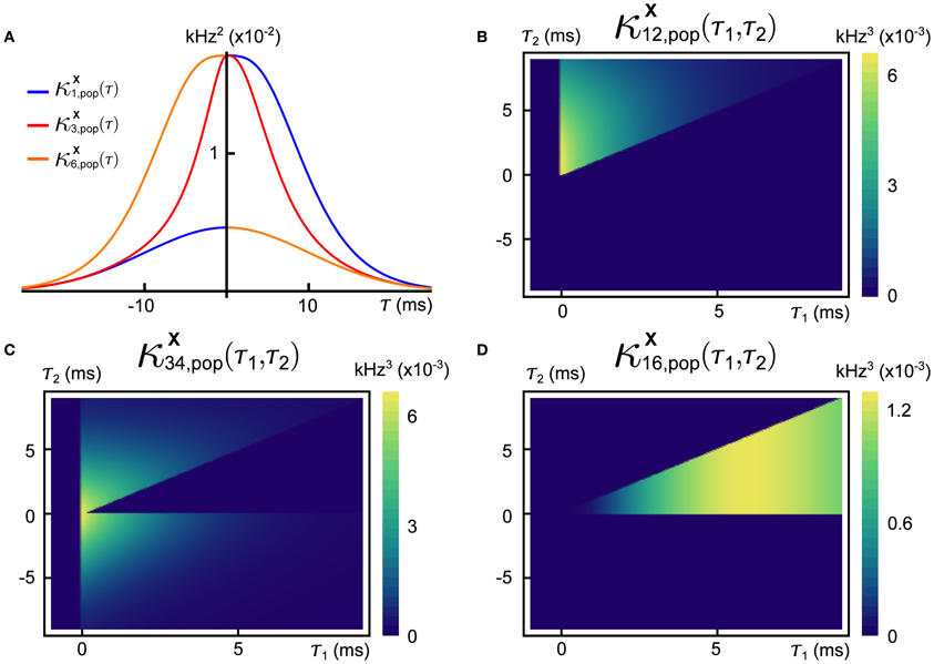
Figure 4. Population cumulants for the synfire-like cascading GTaS process of Figure 3. See Equation (25) for the definition of population cumulants. (A) Second order population cumulant densities for processes 1, 3, and 6. Greater mass to the right (resp. left) of τ = 0 indicates that a cell tends to lead (resp. follow) in pairwise-correlated events. (B) Third order population cumulant for processes X₁, X₂ in the cascading GTaS process. Concentration of the mass in different regions of the plane indicates temporal structure of events correlated between X₁, X₂ relative to the remainder of the population (see the text). (C) Same as (B), but for processes X₃, X₄. (D) Same as (B), but for processes X₁, X₆. System parameters are given in the Appendix.

Greater understanding of the joint temporal statistics in a multivariate counting process can be obtained by considering higher-order population cumulant densities. We define the third-order population cumulant density for the pair (i, j) to be

${\kappa }_{ij,\text{pop}}^X({\tau }_1,{\tau }_2)={\displaystyle \sum _{k\ne i,j}{\kappa }_{ijk}^X}({\tau }_1,{\tau }_2).$

The third-order population cumulant density is linearly related to the spike-triggered population activity, conditioned on spikes in cells i and j separated by a delay τ₁. In Figures 4B–D, we present three distinct third-order population cumulant densities. Examining κ^X_{12, pop}(τ₁, τ₂) (panel B), we see only contributions in the region τ₂ > τ₁ > 0, indicating that the pairwise event 1 → 2 often precedes a third spike elsewhere in the population (i.e., with a probability above chance). The population cumulant κ^X_{34, pop}(τ₁, τ₂) has contributions in two sections of the plane (panel C). Contributions in the region τ₂ > τ₁ > 0 can be understood following the preceding example, while contributions in the region τ₂ < 0 < τ₁ imply that the firing of other neurons tends to precede the joint firing event 3 → 4. Lastly, contributions to κ^X_{16, pop}(τ₁, τ₂) (panel D) are limited to 0 < τ₂ < τ₁, indicating an above chance probability of joint firing events of the form 1→ i → 6, where i indicates a distinct neuron within the population.

A distinct advantage of the study of population cumulant densities as opposed to individual cross-cumulant functions in practical applications is related to data (i.e., sample size) limitations. In many practical applications, where the temporal structure of a collection of observed point processes is of interest, we often deal with a small, noisy samples. It may therefore be difficult to estimate third- or higher-order cumulants. Population cumulants partially circumvent this issue by pooling (Tetzlaff et al., 2003; Rosenbaum et al., 2010, 2011) (or summing) responses, to amplify existing correlations and average out the noise in measurements.

We conclude this section by noting that even cascading GTaS examples can be much more general. For instance, we can include more complex shift patterns, overlapping subassemblies within the population, different temporal processions of the cascade, and more.

2.2.3. Timing-selective network

The responses of single neurons and neuronal networks in experimental (Meister and Berry II, 1999; Singer, 1999; Bathellier et al., 2012) and theoretical studies (Jeffress, 1948; Hopfield, 1995; Joris et al., 1998; Thorpe et al., 2001; Gütig and Sompolinsky, 2006) can reflect the temporal structure of their inputs. Here, we present a simple example that shows how a network can be selective to fine temporal features of its input, and how the GTaS model can be used to explore such examples.

As a general network model, we consider N leaky integrate-and-fire (LIF) neurons with membrane potentials V_i obeying

$\begin{array}{cc}\frac{d{V}_i}{dt}=-V_i+{\displaystyle \sum _{j=1}^N{w}_{ij}}(F\ast z_j)(t)+w^{\text{in}}{x}_i(t),i=1,\dots ,N.& (7)\end{array}$

When the membrane potential of cell i reaches a threshold Vth, an output spike is recorded and the membrane potential is reset to zero, after which evolution of V_i resumes the dynamics in Equation (7). Here w_ij is the synaptic weight of the connection from cell j to i, wⁱⁿ is the input weight, and we assume time to be measured in units of membrane time constants. The function F = τ^{− 1}_syn e^{− (t − τ_d)/τ_syn}Θ(t − τ_d) is a delayed, unit-area exponential synaptic kernel with time-constant τ_syn and delay τ_d. The output of the ith neuron is

$z_i(t)={\displaystyle \sum _j\delta (t-t_i^j),}$

where t^j_i is the time of the jth spike of neuron i. In addition, the input {x_i}^N_{i = 1} is

$x_i(t)={\displaystyle \sum _j\delta (t-s_i^j),}$

where the event times {s^j_i} correspond to those of a GTaS counting process X. Thus, each input spike results in a jump in the membrane potential of the corresponding LIF neuron of amplitude wⁱⁿ. The particular network we consider will have a ring topology (nearest neighbor-only connectivity)—specifically, for i, j = 1, …, N, we let

$w_{ij}=\{\begin{array}{ll}{w}^{\text{syn}}\hfill & i-j\mathrm{mod}N\equiv 1\text{ or }N-1\hfill \\ 0\hfill & \text{otherwise}\hfill \end{array}.$

We further assume that all neurons are excitatory, so that w^syn > 0.

A network of LIF neurons with synaptic delay is a minimal model which can exhibit fine-scale discrimination of temporal patterns of inputs without precise tuning (Izhikevich, 2006) (that is, without being carefully designed to do so, with great sensitivity to modification of network parameters). To exhibit this dependence we generate inputs from two GTaS processes. The first (the cascading model) was described in the preceding example. To independently control the mean and variance of relative shifts we replace the sum of exponential shifts with sums of gamma variates. We also consider a model featuring population-level events without shifts (the synchronous model), where the distribution Q_𝔻 is a δ distribution at zero in all coordinates.

The only difference between the two input models is in the temporal structure of joint events. In particular, the rates, and all long timescale spike count cross-cumulants (equivalent to the total “area” under the cross-cumulant density, see the Methods) of order two and higher are identical for the two processes. We focus on the sensitivity of the network to the temporal cumulant structure of its inputs.

In Figures 5A,B, we present two example rasters of the nearest-neighbor LIF network receiving synchronous (left) and cascading (right) input. In the second case, there is an obvious pattern in the outputs, but the firing rate is also increased. This is quantified in Figure 5C, where we compare the number of output spikes fired by a network receiving synchronous input (horizontal axis) with the same for a network receiving cascading input (vertical axis), over a large number of trials. On average, the cascading input increases the output rate by a factor of 1.5 over the synchronous inputs—we refer to this quantity as the cascade amplification factor (CAF).

FIGURE 5

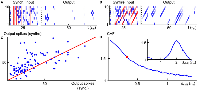
Figure 5. (A) Example input (left) and output (right) for the nearest neighbor LIF network receiving input with synchronous input. (B) Same as (A), but for cascading input. (C) Scatter plot of the output spike count of the network receiving synchronous (horizontal axis) and cascading input (vertical axis) with μ_shift = 2, σ_shift = 0.3. The red line is the diagonal. (D) Average gain (rate in response to cascading input divided by rate in response to synchronous input) as a function of the standard deviation of the gamma variates which compose the shift vectors for population-level events (μ_shift was fixed at 2). The red dot indicates the value of σ_shift used in panel (C). Inset shows the same gain as panel (D), but for varying the mean of the shift distribution (σ_shift = 0.3). Spike counts in panels (C,D) were obtained for trials of length T = 100. Other system parameters are given in the Appendix.

Finally, in Figure 5D, we illustrate how the cascade amplification factor depends on the parameters that define the timing of spikes for the cascading inputs. First, we study the dependence on the standard deviation σ_shift of the gamma variates determining the shift distribution. We note that amplification factors above 1.5 hold robustly (i.e., for a range of shift σ_shift values). The amplification factors decrease with shift variance. In the inset to panel (D), we show how the gain depends on the mean of the shift distribution μ_shift. On an individual trial, the response intensity will depend strongly on the total number of input spikes. Thus, in order to enforce a fair comparison, the mother process and markings used were identical in each trial of every panel of Figure 5. We note that network properties, such as the membrane properties of individual cells or synaptic timescales, may have an equally large impact on the cascade amplification factor—indeed, as we explain below, the observed behavior of the CAF is a result of synergy between the timescales of input and interactions within the network.

These observations have simple explanations in terms of the network dynamics and input statistics. Neglecting, for a moment, population-level events, the network is configured so that correlations in activity decrease with topographic distance. Accordingly, the probability of finding neurons that are simultaneously close to threshold also decreases with distance. Under the synchronous input model, a population-level event results in a simultaneous increase of the membrane potentials of all neurons by an amount wⁱⁿ, but unless the input is very strong (in which case every, or almost every, neuron will fire regardless of fine-scale input structure), the set of neurons sufficiently close to threshold to “capitalize” on the input and fire will typically be restricted to a topographically adjacent subset. Neurons which do not fire almost immediately will soon have forgotten about this population-level input. As a result, the output does not significantly reflect the chain-like structure of the inputs (Figure 5A, right).

On the other hand, in the case of the cascading input, the temporal structure of the input and the timescale of synapses can operate synergistically. Consider a pair of adjacent neurons in the ring network, called cells 1 and 2, arranged so that cell 2 is downstream from cell 1 in the direction of the population-level chain events. When cell 1 spikes, it is likely that cell 2 will also have an elevated membrane potential. The potential is further elevated by the delayed synaptic input from cell 1. If cell 1 spikes in response to a population-level chain event, then cell 2 imminently receives an input spike as well. If the synaptic filter and time-shift of the input spikes to each cell align, then the firing probability of cell 2 will be large relative to chance. This reasoning can be carried on across the network. Hence synergy between the temporal structure of inputs and network architecture allows the network to selectively respond to the temporal structure of the inputs (Figure 5B, right).

In Kuhn et al. (2003), the effect of higher order correlations on the firing rate gain of an integrate-and-fire neuron was studied by driving single cells using sums of SIP or MIP processes with equivalent firing rates (first order cumulants) and pairwise correlations (second order cumulants). In contrast, in the preceding example, the two inputs have equal long time spike count cumulants, and differ only in temporal correlation structure. An increase in firing rate was due to network interactions, and is therefore a population level effect. We return to this comparison in the Discussion.

These examples demonstrate how the GTaS model can be used to explore the impact of spatio-temporal structure in population activity on network dynamics. We next proceed with a formal derivation of the cumulant structure for a general GTaS process.

2.3. Cumulant Structure of a GTaS Process

The GTaS model defines an N-dimensional counting process. Following the standard description for a counting process, X = (X₁, …, X_N) on ℝ^N, given a collection of Borel subsets , i = 1, …, N, then X(A₁ × … × A_N) = (X₁(A₁), …, X_N(A_N)) ∈ ℕ^N is a random vector where the value of each coordinate i indicates the (random) number of points which fall inside the set A_i. Note that the GTaS model defines processes that are marginally Poisson. All GTaS model parameters and related quantities are defined in Table 1.

TABLE 1

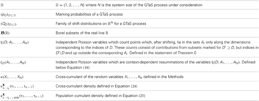
Table 1. Common notation used in the text.

For each D ⊂ 𝔻 = {1, …, N}, define the tail probability ${\overline{p}}_D$ by

$\begin{array}{cc}{\overline{p}}_D={\displaystyle \sum _{D\subset D^{\prime }\subset 𝔻}{p}_{D^{\prime }}.}& (8)\end{array}$

Since p_D is the probability that exactly the processes in D are marked, ${\overline{p}}_D$ is the probability that all processes in D, as well as possibly other processes, are marked. An event from the mother process is assigned to daughter process X_i with probability ${\overline{p}}_{\left\{i\right\}}$. As noted above, an event attributed to process i following a marking D ∋ i will be marginally shifted by a random amount determined by the distribution Q^{i}_D which represents the projection of Q_D onto dimension i. Thus, the events in the marginal process X_i are shifted in an independent and identically distributed (IID) manner according to the mixture distribution Q_i given by

$Q_i=\frac{{\displaystyle {\sum }_{D\ni i}{p}_D{Q}_D^{\left\{i\right\}}}}{{\displaystyle {\sum }_{D\ni i}{p}_D}}.$

Note that IID shifting of the event times of a Poisson process generates another Poisson process of identical rate. Thus, the process X_i is marginally Poisson with rate $\lambda {\overline{p}}_{\left\{i\right\}}$ (Ross, 1995).

In deriving the statistics of the GTaS counting process X, it will be useful to express the distribution of X as

$\begin{array}{cc}\left(\begin{array}{c}{X}_1(A_1)\\ ⋮\\ X_N(A_N)\end{array}\right){=}_{\text{distr}}\left(\begin{array}{c}{\displaystyle {\sum }_{D\ni 1}\xi }(D;A_1,\dots ,A_N)\\ ⋮\\ {\displaystyle {\sum }_{D\ni N}\xi }(D;A_1,\dots ,A_N)\end{array}\right).& (9)\end{array}$

Here, each ξ(D; A₁, …, A_N) is an independent Poisson process, and the notation = _distr indicates that the two random vectors are equal in distribution. This process counts the number of points which are marked by a set D′ ⊃ D, but (after shifting) only the points with indices i ∈ D lie in the corresponding set A_i. Precise definitions of the processes ξ and a proof of Equation (9) may be found in the Appendix. We emphasize that the Poisson processes ξ(D) do not directly count points marked for the set D, but instead points which are marked for a set containing D that, after shifting, only have their D-components lying in the “relevant” sets A_i.

Suppose we are interested in calculating dependencies among a subset of daughter processes, ${\{X_{i_j}\}}_{i_j\in \overline{D}}$ for some set $\overline{D}\subset 𝔻$, consisting of $\left|\overline{D}\right|=k$ distinct members of the collection of counting processes X. Then the following alternative representation will be useful:

$\begin{array}{cc}\left(\begin{array}{c}{X}_{i_1}(A_{i_1})\\ ⋮\\ X_{i_k}(A_{i_k})\end{array}\right){=}_{\text{distr}}\left(\begin{array}{c}{\displaystyle {\sum }_{i_1\in D\subset \overline{D}}{\zeta }_D}(A_1,\dots ,A_N)\\ ⋮\\ {\displaystyle {\sum }_{i_k\in D\subset \overline{D}}{\zeta }_D}(A_1,\dots ,A_N)\end{array}\right)& (10)\end{array}$

where

${\zeta }_D(A_1,\dots ,A_N)={\displaystyle \sum _{\begin{array}{l}{D}^{\prime }\supset D\\ (\overline{D}\backslash D)\cap D^{\prime }=\varnothing \end{array}}\xi (D^{\prime };A_1,\dots ,A_N).}$

We illustrate this decomposition in the cases k = 2, 3 in Figure 6. The sums in Equation (10) run over all sets D ⊂ 𝔻 containing the indicated indices i_j and contained within $\overline{D}$. The processes ζ_D are comprised of a sum of all of the processes ξ(D′) (defined below Equation 9) such that D′ contains all of the indices D, but no other indices which are part of the subset $\overline{D}$ under consideration. These sums are non-overlapping, implying that the ζ_D are also independent and Poisson.

FIGURE 6

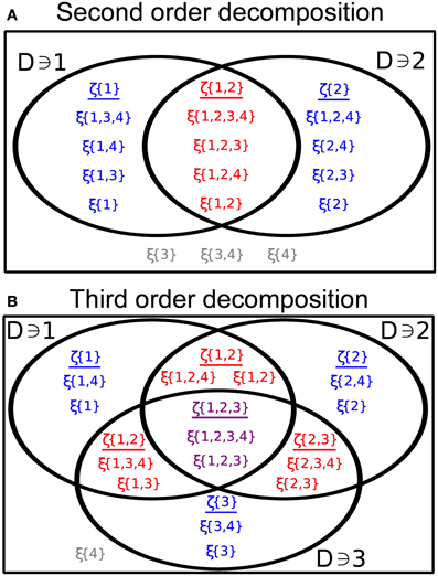
Figure 6. (A) Illustrating the representation given by Equation (10) in the case of two distinct processes (see Equation 11) with N = 4 and $\overline{D}=\{1,2\}$. (B) Same as (A), for three processes with $\overline{D}=\{1,2,3\}$ (see Equation 16).

The following examples elucidate the meaning and significance of Equation (10). We emphasize that the GTaS process is a completely characterized, joint Poisson process, and we use Equation (10) to calculate cumulants of a GTaS process. In principle, any other statistics can be obtained similarly.

2.3.1. Second order cumulants (covariance)

We first generalize a well-known result about the dependence structure of temporally jittered pairs of Poisson processes, X₁, X₂. Assume that events from a mother process with rate λ, are assigned to two daughter processes with probability p. Each event time is subsequently shifted independently according to a univariate distribution f. The cross-cumulant density (or cross-covariance function; see the Methods for cumulant definitions) then has the form (Brette, 2009)

${\kappa }_{12}^X(\tau )=\lambda p{\displaystyle \int f}(t)f(t+\tau )dt=\lambda p(f\times f)(\tau ).$

We generalize this result within the GTaS framework. At second order, Equation (10) has a particularly nice form. Following Bäuerle and Grübel (2005) we write for i ≠ j (see Figure 6A)

$\begin{array}{cc}\left(\begin{array}{c}{X}_i(A_i)\\ X_j(A_j)\end{array}\right){=}_{\text{distr}}\left(\begin{array}{c}{\zeta }_{\{i,j\}}(A_i,A_j)+{\zeta }_{\left\{i\right\}}(A_i)\\ {\zeta }_{\{i,j\}}(A_i,A_j)+{\zeta }_{\left\{j\right\}}(A_j)\end{array}\right).& (11)\end{array}$

The process ζ_{{i, j}} sums all ξ(D′) for which {1, 2} ⊂ D′, while the process ζ_{i} sums all ξ(D′) such that i ∈ D′, j ∉ D′, and ζ_{j} is defined likewise.

Using the representation in Equation (11), we can derive the second order cumulant (covariance) structure of a GTaS process. First, we have

$\begin{array}{l}\mathrm{cov}[X_i(A_i),X_j(A_j)]=\kappa [X_i(A_i),X_j(A_j)]\\ =\kappa [{\zeta }_{\{i,j\}}(A_i,A_j),{\zeta }_{\{i,j\}}(A_i,A_j)]\\ +\kappa [{\zeta }_{\left\{i\right\}}(A_i),{\zeta }_{\{i,j\}}(A_i,A_j)]\\ +\kappa [{\zeta }_{\{i,j\}}(A_i,A_j),{\zeta }_{\left\{j\right\}}(A_j)]\\ +\kappa [{\zeta }_{\left\{i\right\}}(A_i),{\zeta }_{\left\{j\right\}}(A_j)]\\ ={\kappa }_2[{\zeta }_{\{i,j\}}(A_i,A_j)]+0\\ =E[{\zeta }_{\{i,j\}}(A_i,A_j)].\end{array}$

The third equality follows from the construction of the processes ζ_D: if D ≠ D′, then the processes ζ_D, ζ_D′ are independent. The final equality follows from the observation that every cumulant of a Poisson random variable equals its mean.

The covariance may be further expressed in terms of model parameters (see Theorem 1.1 for a generalization of this result to arbitrary cumulant orders):

$\begin{array}{c}\begin{array}{l}\mathrm{cov}[X_i(A_i),X_j(A_j)]\\ =\lambda {\displaystyle \sum _{D^{\prime }\supset \{i,j\}}{p}_{D^{\prime }}}{\displaystyle \int P}\left(t+Y_i\in A_i,t+Y_j\in A_j|Y~Q_{D^{\prime }}\right)dt.\end{array}\end{array}\begin{array}{c} (12)\end{array}$

In other words, the covariance of the counting processes is given by the weighted sum of the probabilities that the (i, j) marginal of the shift distributions yield values in the appropriate sets. The weights are the intensities of each corresponding component processes ξ(D) which contribute events to both of the processes i and j.

In the case that Q_D ≡ Q, Equation (12) reduces to the solution given in Bäuerle and Grübel (2005). Using the tail probabilities defined in Equation (8), if Q_D ≡ Q for all D, the integral in Equation (12) no longer depends on the subset D′, and the equation may be written as

$\begin{array}{l}\mathrm{cov}[X_i(A_i),X_j(A_j)]\\ =\lambda {\overline{p}}_{\{i,j\}}{\displaystyle \int P}\left(t+Y_i\in A_i,t+Y_j\in A_j|Y~Q\right)dt.\end{array}$

Using Equation (12), we may also compute the second cross-cumulant density (also called the covariance density) of the processes. From the definition of the cross-cumulant density [Equation (24) in the Methods], this is given by

$\begin{array}{cc}\begin{array}{l}{\kappa }_{ij}^X(\tau )=\underset{\Delta t\to 0}{\lim }\frac{\mathrm{cov}[X_i([\text{0},\Delta \text{t})),X_j([\tau ,\tau \text{+}\Delta \text{t}))]}{\Delta t^2}\\ =\lambda {\displaystyle \sum _{D^{\prime }\supset \{i,j\}}{p}_{D^{\prime }}}\\ {\displaystyle \int \text{}}\text{}\underset{\Delta t\to 0}{\lim }\text{}\text{}\frac{P(t+Y_i\in [0,\Delta t),t+Y_j\in [\tau ,\tau +\Delta t)|Y~Q_{D^{\prime }})}{\Delta t^2}dt.\end{array}& (13)\end{array}$

Before continuing, we note that given a random vector Y = (Y₁, …, Y_N) ~ Q, where Q has density q(y₁, …, y_N), the vector Z = (Y₂− Y₁, …, Y_N− Y₁) has density q_Z given by

$\begin{array}{cc}{q}_Z({\tau }_1,\dots ,{\tau }_{N-1})={\displaystyle \int q}(t,t+{\tau }_1,\dots ,t+{\tau }_{N-1})dt.& (14)\end{array}$

Assuming that the distributions Q_D′ have densities q_D′, and denoting by q^{{i, j}}_D′ the bivariate marginal density of the variables Y_i, Y_j under Q_D′, we have that

$\begin{array}{cc}{\kappa }_{ij}^X(\tau )=\lambda {\displaystyle \sum _{D^{\prime }\supset \{i,j\}}{p}_{D^{\prime }}}{\displaystyle \int q_{D^{\prime }}^{\{i,j\}}}(t,t+\tau )dt.& (15)\end{array}$

According to Equation (14), the integrals present in Equation (15) are simply the densities of the variables Y_j− Y_i, where Y ~ Q_D′.

Thus κ^X_ij(τ), which captures the additional probability for events in the marginal processes X_i and X_j separated by τ units of time beyond what can be predicted from lower order statistics is given by a weighted sum (in this case, the lower order statistics are marginal intensities—see the discussion around Equation (24) of the Methods). The weights are the “marking rates” λp_D′ for markings contributing events to both component processes, while the summands are the probabilities that the corresponding shift distributions yield a pair of shifts in the proper arrangement—specifically, the shift applied to the event as attributed to X_i precedes that applied to the event mapped to X_j by τ units of time. This interpretation of the cross-cumulant density is quite natural, and will carry over to higher order cross-cumulants of a GTaS process. However, as we show next, this extension is not trivial at higher cumulant orders.

2.3.2. Third order cumulants

To determine the higher order cumulants for a GTaS process, one can again use the representation given in Equation (10). The distribution of a subset of three processes may be expressed in the form (see Figure 6B)

$\begin{array}{cc}\left(\begin{array}{c}{X}_i(A_i)\\ X_j(A_j)\\ X_k(A_k)\end{array}\right){=}_{\text{distr}}\left(\begin{array}{c}{\zeta }_{\{i,j,k\}}+{\zeta }_{\{i,j\}}+{\zeta }_{\{i,k\}}+{\zeta }_{\left\{i\right\}}\\ {\zeta }_{\{i,j,k\}}+{\zeta }_{\{i,j\}}+{\zeta }_{\{j,k\}}+{\zeta }_{\left\{j\right\}}\\ {\zeta }_{\{i,j,k\}}+{\zeta }_{\{i,k\}}+{\zeta }_{\{j,k\}}+{\zeta }_{\left\{k\right\}},\end{array}\right),& (16)\end{array}$

where, for simplicity, we suppressed the arguments of the different ζ_D on the right hand side. Again, the processes in the representation are independent and Poisson distributed. The variable ζ_{{i, j, k}} is the sum of all random variables ξ(D) (see Equation 9) with D ⊃ {i, j, k}, while the variable ζ_{{i, j}} is now the sum of all ξ(D) with D ⊃ {i, j}, but k ∉ D. The rest of the variables are defined likewise. Using properties (C1) and (C2) of cumulants given in the Methods, and assuming that i, j, k are distinct indices, we have

$\kappa (X_i(A_i),X_j(A_j),X_k(A_k))={\kappa }_3({\zeta }_{\{i,j,k\}})=E[{\zeta }_{\{i,j,k\}}].$

The second equality follows from the fact that all cumulants of a Poisson distributed random variable equal its mean. Similar to Equation (12), we may write

$\begin{array}{l}\kappa (X_i(A_i),X_j(A_j),X_k(A_k))\text{}=\text{}\lambda {\displaystyle \sum _{D^{\prime }\supset \{i,j,k\}}{p}_{D^{\prime }}}{\displaystyle \int P}(t+Y_i\in A_i,\\ t+Y_j\in A_j,t+Y_k\in A_k|Y~Q_{D^{\prime }})\text{}dt.\end{array}$

The third cross-cumulant density is then given similarly to the second order function by

${\kappa }_{ijk}^X({\tau }_1,{\tau }_2)=\lambda {\displaystyle \sum _{D^{\prime }\supset \{i,j,k\}}{p}_{D^{\prime }}}{\displaystyle \int q_{D^{\prime }}^{\{i,j,k\}}}(t,t+{\tau }_1,t+{\tau }_2)dt.$

Here, we have again assumed the existence of densities q_D′, and denoted by q^{{i, j, k}}_D′ the joint marginal density of the variables Y_i, Y_j, Y_k under q_D′. The integrals appearing in the expression for the third order cross-cumulant density are the probability densities of the vectors (Y_j− Y_i, Y_k− Y_i), where Y ~ Q_D′.

2.3.3. General cumulants

Finally, consider a general subset of k distinct members of the vector counting process X as in Equation (10). The following theorem provides expressions for the cross-cumulants of the counting processes, as well as the cross-cumulant densities, in terms of model parameters in this general case. The proof of Theorem 1.1 is given in the Appendix.

Theorem 1.1. Let X be a joint counting process of GTaS type with total intensity λ, marking distribution (p_D)_{D ⊂ 𝔻}, and family of shift distributions (Q_D)_{D ⊂ 𝔻}. Let A₁, …, A_k be arbitrary sets in , and $\overline{D}=\{i_1,\dots ,i_k\}\subset 𝔻$ with $\left|\overline{D}\right|=k$. The cross-cumulant of the counting processes may be written

$\begin{array}{cc}\begin{array}{l}\kappa (X_{i_1}(A_1),\dots ,X_{i_k}(A_k))\\ =\lambda {\displaystyle \sum _{D^{\prime }\supset \overline{D}}{p}_{D^{\prime }}}{\displaystyle \int P}(t1+Y^{\overline{D}}\in A_1\times \cdots \times A_k|Y~Q_{D^{\prime }})dt\end{array}& (17)\end{array}$

where $Y^{\overline{D}}$ represents the projection of the random vector Y onto the dimensions indicated by the members of the set $\overline{D}$. Furthermore, assuming that the shift distributions possess densities (q_D)_{D ⊂ 𝔻}, the cross-cumulant density is given by

$\begin{array}{cc}\begin{array}{l}{\kappa }_{i_1\cdots i_k}^X({\tau }_1,\dots ,{\tau }_{k-1})\\ =\lambda {\displaystyle \sum _{D^{\prime }\supset \overline{D}}{p}_{D^{\prime }}}{\displaystyle \int q_{D^{\prime }}^{\overline{D}}}(t,t+{\tau }_1,\cdots ,t+{\tau }_{k-1})dt,\end{array}& (18)\end{array}$

where $q_{D^{\prime }}^{\overline{D}}$ indicates the kth order joint marginal density of q_D′ in the dimensions of $\overline{D}$.

An immediate corollary of Theorem 1.1 is a simple expression for the infinite-time-window cumulants, obtained by integrating the cumulant density across all time lags τ_i. From Equation (A8), we have

$\begin{array}{cc}\begin{array}{l}{\gamma }_{i_1\cdots i_k}^X(\infty )={\displaystyle \int \cdots }{\displaystyle \int {\kappa }_{i_1\cdots i_k}^X}({\tau }_1,\dots ,{\tau }_{k-1})d{\tau }_{k-1}\cdots d{\tau }_1\\ =\lambda {\displaystyle \sum _{D^{\prime }\supset \overline{D}}{p}_{D^{\prime }}}·1=\lambda {\overline{p}}_{\overline{D}}.\end{array}& (19)\end{array}$

This shows that the infinite time window cumulants for a GTaS process are non-increasing with respect to the ordering of sets, i.e.,

${\gamma }_{i_1\cdots i_k}^X(\infty )\ge {\gamma }_{i_1\cdots i_k{i}_{k+1}}^X(\infty ).$

We conclude this section with a short technical remark: Until this point, we have considered only the cumulant structure of sets of unique processes. However occasionally, one may wish to calculate a cumulant for a set of processes including repeats. Take, for example, a cumulant κ(X₁(A₁), X₁(A₂), X₃(A₃)). Owing to the marginally Poisson nature of the GTaS process, we would have (referring to the Methods for cumulant definitions)

$\begin{array}{cc}\begin{array}{l}\kappa (X_1(A_1),X_1(A_2),X_3(A_3))\\ ={\kappa }_{(2,1)}(X_1(A_1\cap A_2),X_3(A_3))\text{if}X~\text{GTaS}.\end{array}& (20)\end{array}$

For a general counting process X, it may be shown that

$\begin{array}{cc}{\kappa }_{113}^X({\tau }_1,{\tau }_2)=\delta ({\tau }_1){\kappa }_{13}^X({\tau }_2)+“\text{non-singular contributions}”.& (21)\end{array}$

In addition, the second order auto-cumulant density may be written (Cox and Isham, 1980)

${\kappa }_{ii}^X(\tau )=r_i\delta (\tau )+“\text{non-singular contributions}”,$

where r_i is the stationary rate. The singular contribution shown in Equation (21) at third order is in analogy to the delta contribution proportional to the firing rate which appears in the second-order auto-cumulant density. For a GTaS process, the non-singular contributions in Equation (21) are identically zero, following directly from Equation (20). Expressions similar to Equations (20, 21) hold for general cases.

3. Discussion

We have introduced a general method of generating spike trains with flexible spatiotemporal structure. The GTaS model is completely analytically tractable: all statistics of interest can be obtained directly from the distributions used to define it. It is based on an intuitive method of selecting and shifting point processes from a “mother” train. Moreover, the GTaS model can be used to easily generate partially synchronous states, cluster firing, cascading chains, and other spatiotemporal patterns of neural activity.

Processes generated by the GTaS model are naturally described by cumulant densities of pairwise and higher orders. This raises the question of whether such statistics are readily computable from data, so that realistic classes of GTaS models can be defined in the first place. One approach is to fit mechanistic models to data, and to use the higher order structure that is generated by the underlying mechanisms (Yu et al., 2011). A synergistic blend of other methods with the GTaS framework may also be fruitful—for example, the CuBIC framework of Staude et al. (2010) could be used to determine relevant marking orders, and the parametrically-described GTaS process could then be fit to allow generation of surrogate data after selection of appropriate classes of shift distributions. When it is necessary to infer higher order structure in the face of data limitations, population cumulants are an option to increase statistical power (albeit at the cost of spatial resolution; see Figure 4).

While the GTaS model has flexible higher order structure, it is always marginally Poisson. While throughout the cortex spiking is significantly irregular (Holt et al., 1996; Shadlen and Newsome, 1998), the level of variability differs across cells, with Fano factors ranging from below 0.5 to above 1.5—in comparison with the Poisson value of 1 (Churchland et al., 2010). Changes in variability may reflect cortical states and computation (Litwin-Kumar and Doiron, 2012; White et al., 2012). A model that would allow flexible marginal variability would therefore be very useful. Unfortunately, the tractability of the GTaS model is closely related to the fact that the marginal processes are Poisson. Therefore an immediate generalization does not seem possible.

A number of other models have been used to describe population activity. Maximum entropy (ME) approaches also result in models with varied spatial activity; these are defined based on moments or other averaged features of multivariate spiking activity (Schneidman et al., 2006; Roudi et al., 2009). Such models are often used to fit purely spatial patterns of activity, though (Tang et al, 2008; Marre et al., 2009) have extended the techniques to treat temporal correlations as well. Generalized linear models (GLMs) have been used successfully to describe spatiotemporal patterns at second (Pillow et al., 2008), and third order (Ohiorhenuan et al., 2010). In comparison to the present GTaS method, both GLMs and ME models are more flexible. They feature well-defined approaches for fitting to data, including likelihood-based methods with well-behaved convexity properties. What the GTaS method contributes is an explicit way to generate population activity with explicitly specified high order spatio-temporal structure. Moreover, the lower order cumulant structure of a GTaS process can be modified independently of the higher order structure, though the reverse is not true.

There are a number of possible implications of such spatio-temporal structure for communication within neural networks. In section 2.2.3, we showed that these temporal correlations can play a role similar to that of spatial correlations established in Kuhn et al. (2003) for determining network input-output transfer. Our model allowed us to examine that impact of such temporal correlations on the network-level gain of a downstream population (cascade amplification factor). Even in a very simple network it was clear that the strength of the response is determined jointly by the temporal structure of the input to the network, and the connectivity within the network. Kuhn et al. examined the effect of higher order structure on the firing rate gain of an integrate-and-fire neuron by driving it with a mixture of SIP or MIP processes (Kuhn et al., 2003). However, in these studies, only the spatial structure of higher order activity was varied. The GTaS model allows us to concurrently change the temporal structure of correlations. In addition, the precise control of the cumulants allows us to derive models which are equivalent up to a certain cross-cumulant order, when the configuration of marking probabilities and shift distributions allow it (as for the SIP and MIP processes of Kuhn et al. (2003), which are equivalent at second order).

Such patterns of activity may be useful when experimentally probing dendritic information processing (Gasparini and Magee, 2006), synaptic plasticity (Pfister and Gerstner, 2006; Gjorgjieva et al., 2011), or investigating the response of neuronal networks to complex patterns of input (Kahn et al., 2013). Spatiotemporal patterns may also be generated by cell assemblies (Bathellier et al., 2012). The firing in such assemblies can be spatially structured, and this structure may not be reflected in the activity of participating cells. Assemblies can exhibit persistent patterns of firing, sometimes with millisecond precision (Harris et al., 2002). The GTaS framework is well suited to describe exactly such activity patterns. The examples we presented can be easily extended to generate more complex patterns of activity with overlapping cell assemblies, different cells leading the activity, and other variations.

Understanding impact of spatiotemporal patterns on neural computations remains an open and exciting problem. Progress will require coordination of computational, theoretical, and experimental work—the latter taking advantage of novel stimulation techniques. We hope that the GTaS model, as a practical and flexible method for generating high-dimensional, correlated spike trains, will play a significant role along the way.

4. Methods

4.1. Cumulants as a Measure of Dependence

We first define cross-cumulants (also called joint cumulants) (Stratonovich and Silverman, 1967; Kendall et al., 1969; Gardiner, 2009) and review some important properties of these quantities. Define the cumulant generating function g of a random vector X = (X₁, …, X_N) by

$g(t_1,\dots ,t_N)=\log \left(E\left[\exp \left({\displaystyle \sum _{j=1}^N{t}_j}{X}_j\right)\right]\right).$

The r-cross-cumulant of the vector X is given by

${\kappa }_r(X)=\frac{{\partial }^{\left|r\right|}}{\partial t_1^{r_1}\cdots \partial t_N^{r_N}}g(t_1,\dots ,t_N){|}_{t_1=\cdots =t_N=0}.$

where r = (r₁, …, r_N) is a N-vector of positive integers, and |r| = ∑^N_{i = 1} r_i. We will generally deal with cumulants where all variables are considered at first order, without excluding the possibility that some variables are duplicated. In this case, we define the cross-cumulant κ(X), of the variables in the random vector X = (X₁, …, X_N) as

$\begin{array}{l}\kappa (X):={\kappa }_1(X)=\frac{{\partial }^N}{\partial t_1\cdots \partial t_N}g(t_1,\dots ,t_N){|}_{t_1=\cdots =t_N=0}\\ \text{where}1=(1,\dots ,1).\end{array}$

This relationship may be expressed in combinatorial form:

$\begin{array}{cc}\kappa (X_1,\dots ,X_N)={{\displaystyle \sum _{\pi }(|\pi |-1)!(-1)}}^{\left|\pi \right|-1}{\displaystyle \prod _{B\in \pi }E\left[{\displaystyle \prod _{i\in B}{X}_i}\right]}& (22)\end{array}$

where π runs through all partitions of 𝔻 = {1, …, N}, and B runs over all blocks in a partition π. More generally, the r-cross-cumulant may be expressed in terms of moments by expanding the cumulant generating function as a Taylor series, noting that

$\begin{array}{l}g(t_1,\dots ,t_N)={\displaystyle \sum _r\frac{{\kappa }_r(X_1,\dots ,X_N)}{r!}{x}_1^{r_1}\cdots x_d^{r_N}}\text{with}\\ r!={\displaystyle \prod _{i=1}^N{r}_i!,}\end{array}$

similarly expanding the moment generating function M(t) = e^g(t), and matching the polynomial coefficients. Note that the nth cumulant κ_n of a random variable X may be expressed as a joint cumulant via

${\kappa }_n(X)=\kappa \underset{\text{n copies of }X}{\underbrace{(X,\dots ,X)}}.$

We will utilize the following two principal properties of cumulants (Brillinger, 1965; Stratonovich and Silverman, 1967; Mendel, 1991; Staude et al., 2010):

(C1) Multilinearity - for any random variables X, Y, {Z_i}^N_{i = 2}, we have

$\begin{array}{l}\kappa (aX+bY,Z_2,\dots ,Z_N)=a\kappa (X,Z_2,\dots ,Z_N)\\ +b\kappa (Y,Z_2,\dots ,Z_N).\end{array}$

This holds regardless of dependencies amongst the random variables.

(C2) If any subset of the random variables in the cumulant argument is independent from the remaining, the cross-cumulant is zero—i.e., if {X₁, …, X_N1} and {Y₁, …, Y_N2} are sets of random variables such that each X_i is independent from each Y_j, then

$\begin{array}{l}{\kappa }_{(r_X,r_Y)}(X_1,\dots ,X_{N_1},Y_1,\dots ,Y_{N_2})=0\\ \text{for all}{r}_X\in {\mathbb{N}}_{+}^{N_1},r_Y\in {\mathbb{N}}_{+}^{N_2}.\end{array}$

To exhibit another key property of cumulants, consider a 4-vector X = (X₁, X₂, X₃, X₄) with non-zero fourth cumulant and a random variable Z independent of each X_i. Define Y = (X₁ + Z, X₂ + Z, X₃ + Z, X₄). Using properties (C1), (C2) above, it follows that

$\kappa (Y_1,Y_2,Y_3)=\kappa (X_1,X_2,X_3)+{\kappa }_3(Z).$

On the other hand, it is also true that

$\kappa (Y)=\kappa (X),$

that is, adding the variable Z to only a subset of the variables in X results in changes to cumulants involving only that subset, but not to the joint cumulant of the entire vector. In this sense, an rth order cross-cumulant of a collection of random variables captures exclusively dependencies amongst the collection which cannot be described by cumulants of lower order. In the example above, only the joint statistical properties of a subset of X were changed. As a result, the total cumulant κ(X) remained fixed.

From Equation (22), it is apparent that κ(X_i) = E[X_i], and κ(X_i, X_j) = cov[X_i, X_j]. In addition, the third cumulant, like the second, is equal to the corresponding central moment:

$\kappa (X_i,X_j,X_k)=E[(X_i-E[X_i])(X_j-E[X_j])(X_k-E[X_k])].$

As cumulants and central moments agree up to third order, central moments up to third order inherit the properties discussed above at these orders. On the other hand, the fourth cumulant is not equal to the fourth central moment. Rather:

$\begin{array}{cc}\begin{array}{l}\kappa (X_i,X_j,X_k,X_l)\\ =E[(X_i-E[X_i\text{]})(X_j-E[X_j])(X_k-E[X_k])(X_l-E[X_l])]\\ -\mathrm{cov}[X_i,X_j]\mathrm{cov}[X_k,X_l]-\mathrm{cov}[X_i,X_k]\mathrm{cov}[X_j,X_l]\\ -\mathrm{cov}[X_i,X_l]\mathrm{cov}[X_j,X_k].\end{array}& (23)\end{array}$

Higher cumulants have similar (but more complicated) expansions in terms of central moments. Accordingly, central moments of fourth and higher order do not inherit properties (C1), (C2).

4.2. Temporal Statistics of Point Processes

In the Results, we present an extension of previous work (Bäuerle and Grübel, 2005) in which we construct and analyze multivariate counting processes X = (X₁, …, X_N) where each X_i is marginally Poisson.

Formally, a counting process X is an integer-valued random measure on . Evaluated on subset A₁ × … × A_N of , the random vector (X₁(A₁), …, X_N(A_N)) counts events in d distinct categories whose times of occurrence fall in to the sets A_i. A good general reference on the properties of counting processes (marginally Poisson and otherwise) is Daley and Vere-Jones (2002).

The assumption of Poisson marginals implies that for a set , the random variable X_i(A_i) follows a Poisson distribution with mean λ_i ℓ(A_i), where ℓ is the Lebesgue measure on ℝ, and λ_i is the (constant) rate for the ith process. The processes under consideration will further satisfy a joint stationarity condition, namely that the distribution of the vector (X₁(A₁ + t), …, X_N(A_N + t)) does not depend on t, where A_i + t denotes the translated set {a + t : a ∈ A_i}.

We now consider some common measures of temporal dependence for jointly stationary vector counting processes. We will refer to the quantity X_i[0, T] as the spike count of process i over [0, T]. The quantity γ^X_{i1… ik}(T) (which we will refer to as a spike count cumulant) is given by

${\gamma }_{i_1\cdots i_k}^X(T)=\frac{1}{T}\kappa [X_{i_1}[0,T],\dots ,X_{i_k}[0,T]]$

measures kth order correlations amongst spike counts for the listed processes which occur over windows of length T. At second order, γ^X_ij(T) measures the covariance of the spike counts of processes i, j over a common window of length T. The infinite window spike count cumulant quantifies dependencies in the spike counts of point processes over arbitrarily long windows, and is given by

${\gamma }_{i_1\cdots i_k}^X(\infty )=\underset{T\to \infty }{\lim }{\gamma }_{i_1\cdots i_k}^X(T).$

A related measure is the kth order cross-cumulant density κ^X_{i1, …, ik}(τ₁, …, τ_{k − 1}), defined by

$\begin{array}{cc}\begin{array}{l}{\kappa }_{i_1\cdots i_k}^X({\tau }_1,\dots ,{\tau }_{k-1})=\underset{\Delta t\to 0}{\lim }\frac{1}{\Delta t^k}\kappa [X_{i_1}[0,\Delta t],\\ X_{i_2}[{\tau }_1,{\tau }_1+\Delta t],\dots ,X_{i_k}[{\tau }_{k-1},{\tau }_{k-1}+\Delta t]].\end{array}& (24)\end{array}$

The cross-cumulant density should be interpreted as a measure of the likelihood—above what may be expected from knowledge of the lower order cumulant structure—of seeing events in processes i₂, …, i_k at times τ₁ + t, …, τ_{k − 1} + t, conditioned on event in process i₁ at time t. The infinite window spike count cumulant is equal to the total integral under the cross-cumulant density,

${\gamma }_{i_1\cdots i_k}^X(\infty )={\displaystyle \int \cdots }{\displaystyle \int {\kappa }_{i_1\cdots i_k}^X}({\tau }_1,\dots ,{\tau }_{k-1})d{\tau }_{k-1}\cdots d{\tau }_1.$

As an example, we again consider the familiar second-order cross-cumulant density κ^X_ij(τ)—often referred to as the cross-covariance density or cross-correlation function. Defining the conditional intensity h_ij(τ) of process j, conditioned on process i to be

$h_{ij}^X(\tau )=\underset{\Delta t\to 0}{\lim }\frac{1}{\Delta t}P(X_j[\tau ,\tau +\Delta t]>0|X_i[0,\Delta t]>0),$

that is, the intensity of j conditioned on an event in process i which occurred τ units of time in the past, then it is not difficult to show that

${\kappa }_{ij}^X(\tau )={\lambda }_i{h}_{ij}(\tau )-{\lambda }_i{\lambda }_j.$

That is, the second order cross-cumulant density supplies the probability of chance of observing an event attributed to process i, followed by one attributed to process j, τ units of time later, above what would be expected from knowledge of first order statistics (given by the product of the marginal intensities, λ_i λ_j). More generally, at higher orders, the cross-cumulant density should be interpreted as a measure of the likelihood (above what may be expected from knowledge of the lower order correlation structure) of seeing events attribute to processes i₂, …, i_k at times τ₁ + t, …, τ_{k − 1} + t, conditioned on an event in process i₁ at time t.

Another statistic useful in the study of a correlated vector counting process X is the population cumulant density. At second-order, the population cumulant density for X_i takes the form (Luczak et al., 2013)

${\kappa }_{i,\text{pop}}^X(\tau )={\displaystyle \sum _{j\ne i}{\kappa }_{ij}^X}(\tau ).$

More generally, the kth order population cumulant density corresponding to the processes X_i1, …, X_{ik − 1} is given by

$\begin{array}{c}{\kappa }_{i_1\cdots i_{k-1},\text{pop}}^X({\tau }_1,\dots ,{\tau }_{k-1})={\displaystyle \sum _{j\ne i_1,\dots ,i_k}{\kappa }_{i_1\cdots i_{k-1}j}^X}({\tau }_1,\dots ,{\tau }_{k-1}).\end{array}\begin{array}{c} (25)\end{array}$

Funding

This work was supported by NSF grants DMS-0817649, DMS-1122094, a Texas ARP/ATP award to Krešimir Josić, and by a Career Award at the Scientific Interface from the Burroughs Wellcome Fund and NSF Grant DMS-1122106 to Eric Shea-Brown.

Conflict of Interest Statement

The authors declare that the research was conducted in the absence of any commercial or financial relationships that could be construed as a potential conflict of interest.

References

Abeles, M. (1991). Corticonics: Neural Circuits of the Cerebral Cortex. Cambridge: Cambridge University Press. doi: 10.1017/CBO9780511574566

CrossRef Full Text

Abeles, M., and Prut, Y. (1996). Spatio-temporal firing patterns in the frontal cortex of behaving monkeys. J. Physiol. Paris 90, 249–250. doi: 10.1016/S0928-4257(97)81433-7

Pubmed Abstract | Pubmed Full Text | CrossRef Full Text

Aertsen, A., Diesmann, M., and Gewaltig, M. O. (1996). Propagation of synchronous spiking activity in feedforward neural networks. J. Physiol. Paris 90, 243–247. doi: 10.1016/S0928-4257(97)81432-5

Pubmed Abstract | Pubmed Full Text | CrossRef Full Text

Amari, S., Nakahara, H., Wu, S., and Sakai, Y. (2003). Synchronous firing and higher-order interactions in neuron pool. Neural Comput. 15, 127–142. doi: 10.1162/089976603321043720

Pubmed Abstract | Pubmed Full Text | CrossRef Full Text

Amjad, A. M., Halliday, D. M., Rosenberg, J. R., and Conway, B. A. (1997). An extended difference of coherence test for comparing and combining several independent coherence estimates: theory and application to the study of motor units and physiological tremor. J. Neurosci. Meth. 73, 69–79. doi: 10.1016/S0165-0270(96)02214-5

Pubmed Abstract | Pubmed Full Text | CrossRef Full Text

Averbeck, B. B., Latham, P. E., and Pouget, A. (2006). Neural correlations, population coding and computation. Nat. Rev. Neurosci. 7, 358–366. doi: 10.1038/nrn1888

Pubmed Abstract | Pubmed Full Text | CrossRef Full Text

Aviel, Y., Pavlov, E., Abeles, M., and Horn, D. (2002). Synfire chain in a balanced network. Neurocomputing 44, 285–292. doi: 10.1016/S0925-2312(02)00352-1

CrossRef Full Text

Bair, W., Zohary, E., and Newsome, W. (2001). Correlated firing in macaque visual area mt: time scales and relationship to behavior. J. Neurosci. 21, 1676–1697.

Pubmed Abstract | Pubmed Full Text

Barreiro, A. K., Shea-Brown, E., and Thilo, E. L. (2010). Time scales of spike-train correlation for neural oscillators with common drive. Phys. Rev. E 81:011916. doi: 10.1103/PhysRevE.81.011916

Pubmed Abstract | Pubmed Full Text | CrossRef Full Text

Bathellier, B., Ushakova, L., and Rumpel, S. (2012). Discrete neocortical dynamics predict behavioral categorization of sounds. Neuron 76, 435–449. doi: 10.1016/j.neuron.2012.07.008

Pubmed Abstract | Pubmed Full Text | CrossRef Full Text

Bäuerle, N., and Grübel, R. (2005). Multivariate counting processes: copulas and beyond. Astin Bull. 35, 379. doi: 10.2143/AST.35.2.2003459

CrossRef Full Text

Branco, T., Clark, B. A., and Hausser, M. (2010). Dendritic discrimination of temporal input sequences in cortical neurons. Sci. Signal. 329, 1671. doi: 10.1126/science.1189664

Pubmed Abstract | Pubmed Full Text | CrossRef Full Text

Branco, T., and Häusser, M. (2011). Synaptic integration gradients in single cortical pyramidal cell dendrites. Neuron 69, 885–892. doi: 10.1016/j.neuron.2011.02.006

Pubmed Abstract | Pubmed Full Text | CrossRef Full Text

Brette, R. (2009). Generation of correlated spike trains. Neural Comput. 21, 188–215. doi: 10.1162/neco.2009.12-07-657

Pubmed Abstract | Pubmed Full Text | CrossRef Full Text

Brillinger, D. R. (1965). An introduction to polyspectra. Ann. Math. Stat. 36, 1351–1374. doi: 10.1214/aoms/1177699896

CrossRef Full Text

Buzsáki, G. (2010). Neural syntax: cell assemblies, synapsembles, and readers. Neuron 68, 362–385. doi: 10.1016/j.neuron.2010.09.023

Pubmed Abstract | Pubmed Full Text | CrossRef Full Text

Cain, N., and Shea-Brown, E. (2013). Impact of correlated neural activity on decision-making performance. Neural Comput. 25, 289–327. doi: 10.1162/NECO_a_00398

Pubmed Abstract | Pubmed Full Text | CrossRef Full Text

Carr, C. E., Agmon-Snir, H., and Rinzel, J. (1998). The role of dendrites in auditory coincidence detection. Nature 393, 268–272. doi: 10.1038/30505

Pubmed Abstract | Pubmed Full Text | CrossRef Full Text

Chow, B. Y., Han, X., Dobry, A. S., Qian, X., Chuong, A. S., Li, M., et al. (2010). High-performance genetically targetable optical neural silencing by light-driven proton pumps. Nature 463, 98–102. doi: 10.1038/nature08652

Pubmed Abstract | Pubmed Full Text | CrossRef Full Text

Churchland, M. M., Yu, B. M., Cunningham, J. P., Sugrue, L. P., Cohen, M. R., Corrado, G. S., et al. (2010). Stimulus onset quenches neural variability: a widespread cortical phenomenon. Nat. Neurosci. 13, 369–378. doi: 10.1038/nn.2501

Pubmed Abstract | Pubmed Full Text | CrossRef Full Text

Cox, D. R., and Isham, V. (1980). Point Processes. Vol. 12. London: Chapman and Hall/CRC.

Daley, D. J., and Vere-Jones, D. (2002). An Introduction to the Theory of Point Processes: Volume I: Elementary Theory and Methods. Vol. 1. New York, NY: Springer.

Ganmor, E., Segev, R., and Schneidman, E. (2011). Sparse low-order interaction network underlies a highly correlated and learnable neural population code. Proc. Natl. Acad. Sci. U.S.A. 108, 9679–9684. doi: 10.1073/pnas.1019641108

Pubmed Abstract | Pubmed Full Text | CrossRef Full Text

Gardiner, C. W. (2009). Handbook of Stochastic Methods for Physics, Chemistry and the Natural Sciences. Berlin: Springer-Verlag.

Gasparini, S., and Magee, J. C. (2006). State-dependent dendritic computation in hippocampal CA1 pyramidal neurons. J. Neurosci. 26, 2088–2100. doi: 10.1523/JNEUROSCI.4428-05.2006

Pubmed Abstract | Pubmed Full Text | CrossRef Full Text

Gjorgjieva, J., Clopath, C., Audet, J., and Pfister, J.-P. (2011). A triplet spike-timing–dependent plasticity model generalizes the bienenstock–cooper–munro rule to higher-order spatiotemporal correlations. Proc. Natl. Acad. Sci. U.S.A. 108, 19383–19388. doi: 10.1073/pnas.1105933108

Pubmed Abstract | Pubmed Full Text | CrossRef Full Text

Grün, S., and Rotter, S. (2010). Analysis of Parallel Spike Trains. New York, NY: Springer. doi: 10.1007/978-1-4419-5675-0

CrossRef Full Text

Gütig, R., and Sompolinsky, H. (2006). The tempotron: a neuron that learns spike timing–based decisions. Nat. Neurosci. 9, 420–428. doi: 10.1038/nn1643

Pubmed Abstract | Pubmed Full Text | CrossRef Full Text

Gutnisky, D. A., and Josić, K. (2009). Generation of spatio-temporally correlated spike-trains and local-field potentials using a multivariate autoregressive process. J. Neurophysiol. 103, 2912–2930. doi: 10.1152/jn.00518.2009

Pubmed Abstract | Pubmed Full Text | CrossRef Full Text

Han, X., and Boyden, E. S. (2007). Multiple-color optical activation, silencing, and desynchronization of neural activity, with single-spike temporal resolution. PLoS ONE 2:e299. doi: 10.1371/journal.pone.0000299

Pubmed Abstract | Pubmed Full Text | CrossRef Full Text

Hansen, B. J., Chelaru, M. I., and Dragoi, V. (2012). Correlated variability in laminar cortical circuits. Neuron 76, 590–602. doi: 10.1016/j.neuron.2012.08.029

Pubmed Abstract | Pubmed Full Text | CrossRef Full Text

Harris, K. D. (2005). Neural signatures of cell assembly organization. Nat. Rev. Neurosci. 6, 399–407. doi: 10.1038/nrn1669

Pubmed Abstract | Pubmed Full Text | CrossRef Full Text

Harris, K. D., Henze, D. A., Hirase, H., Leinekugel, X., Dragoi, G., Czurkó, A., et al. (2002). Spike train dynamics predicts theta-related phase precession in hippocampal pyramidal cells. Nature 417, 738–741. doi: 10.1038/nature00808

Pubmed Abstract | Pubmed Full Text | CrossRef Full Text

Hebb, D. O. (1949). The Organization of Behavior: A Neuropsychological Theory. New York, NY: Psychology Press.

Holt, G. R., Softky, W. R., Koch, C., and Douglas, R. J. (1996). Comparison of discharge variability in vitro and in vivo in cat visual cortex neurons. J. Neurophysiol. 75, 1806–1814.

Pubmed Abstract | Pubmed Full Text

Hopfield, J. J. (1995). Pattern recognition computation using action potential timing for stimulus representation. Nature 376, 33–36. doi: 10.1038/376033a0

Pubmed Abstract | Pubmed Full Text | CrossRef Full Text

Ikegaya, Y., Aaron, G., Cossart, R., Aronov, D., Lampl, I., Ferster, D., et al. (2004). Synfire chains and cortical songs: temporal modules of cortical activity. Sci. Signal. 304, 559. doi: 10.1126/science.1093173

Pubmed Abstract | Pubmed Full Text | CrossRef Full Text

Izhikevich, E. M. (2006). Polychronization: computation with spikes. Neural Comput. 18, 245–282. doi: 10.1162/089976606775093882

Pubmed Abstract | Pubmed Full Text | CrossRef Full Text

Jeffress, L. A. (1948). A place theory of sound localization. J. Comp. Physiol. Psychol. 41, 35–39. doi: 10.1037/h0061495

Pubmed Abstract | Pubmed Full Text | CrossRef Full Text

Johnson, D. H., and Goodman, I. N. (2009). Jointly Poisson processes. arXiv preprint arXiv:0911.2524.

Joris, P. X., Smith, P. H., and Yin, T. C. T. (1998). Coincidence detection in the auditory system: 50 years after Jeffress. Neuron 21, 1235–1238. doi: 10.1016/S0896-6273(00)80643-1

Pubmed Abstract | Pubmed Full Text | CrossRef Full Text

Kahn, I., Knoblich, U., Desai, M., Bernstein, J., Graybiel, A. M., Boyden, E. S., et al. (2013). Optogenetic drive of neocortical pyramidal neurons generates fMRI signals that are correlated with spiking activity. Brain Res. 1511, 33–45. doi: 10.1016/j.brainres.2013.03.011

Pubmed Abstract | Pubmed Full Text | CrossRef Full Text

Kendall, M. G., Stuart, A., and Ord, J. K. (1969). The Advanced Theory of Statistics. Vol. 1, 3rd Edn. London: Griffin.

Köster, U., Sohl-Dickstein, J., Gray, C. M., and Olshausen, B. A. (2013). Higher order correlations within cortical layers dominate functional connectivity in microcolumns. arXiv preprint arXiv:1301.0050.

Krumin, M., and Shoham, S. (2009). Generation of spike trains with controlled auto- and cross-correlation functions. Neural Comput. 21, 1642–1664. doi: 10.1162/neco.2009.08-08-847

Pubmed Abstract | Pubmed Full Text | CrossRef Full Text

Kuhn, A., Aertsen, A., and Rotter, S. (2003). Higher-order statistics of input ensembles and the response of simple model neurons. Neural Comput. 15, 67–101. doi: 10.1162/089976603321043702

Pubmed Abstract | Pubmed Full Text | CrossRef Full Text

Litwin-Kumar, A., and Doiron, B. (2012). Slow dynamics and high variability in balanced cortical networks with clustered connections. Nat. Neurosci. 15, 1498–1505. doi: 10.1038/nn.3220

Pubmed Abstract | Pubmed Full Text | CrossRef Full Text

Luczak, A., Bartho, P., and Harris, K. D. (2013). Gating of sensory input by spontaneous cortical activity. J. Neurosci. 33, 1684–1695. doi: 10.1523/JNEUROSCI.2928-12.2013

Pubmed Abstract | Pubmed Full Text | CrossRef Full Text

Luczak, A., Barthó, P., Marguet, S. L., Buzsáki, G., and Harris, K. D. (2007). Sequential structure of neocortical spontaneous activity in vivo. Proc. Natl. Acad. Sci. U.S.A. 104, 347–352. doi: 10.1073/pnas.0605643104

Pubmed Abstract | Pubmed Full Text | CrossRef Full Text

Macke, J. H., Berens, P., Ecker, A. S., Tolias, A. S., and Bethge, M. (2009). Generating spike trains with specified correlation coefficients. Neural Comput. 21, 397–423. doi: 10.1162/neco.2008.02-08-713

Pubmed Abstract | Pubmed Full Text | CrossRef Full Text

Macke, J. H., Opper, M., and Bethge, M. (2011). Common input explains higher-order correlations and entropy in a simple model of neural population activity. Phys. Rev. Lett. 106:208102. doi: 10.1103/PhysRevLett.106.208102

Pubmed Abstract | Pubmed Full Text | CrossRef Full Text

Marre, O., El Boustani, S., Frégnac, Y., and Destexhe, A. (2009). Prediction of spatiotemporal patterns of neural activity from pairwise correlations. Phys. Rev. Lett. 102:138101. doi: 10.1103/PhysRevLett.102.138101

Pubmed Abstract | Pubmed Full Text | CrossRef Full Text

Meister, M., and Berry II, M. J. (1999). The neural code of the retina. Neuron 22, 435. doi: 10.1016/S0896-6273(00)80700-X

Pubmed Abstract | Pubmed Full Text | CrossRef Full Text

Mendel, J. M. (1991). Tutorial on higher-order statistics (spectra) in signal processing and system theory: theoretical results and some applications. Proc. IEEE 79, 278–305. doi: 10.1109/5.75086

CrossRef Full Text

Montani, F., Phoka, E., Portesi, M., and Schultz, S. R. (2013). Statistical modelling of higher-order correlations in pools of neural activity. Physica A 392, 3066–3086. doi: 10.1016/j.physa.2013.03.012

CrossRef Full Text

Ohiorhenuan, I. E., Mechler, F., Purpura, K. P., Schmid, A. M., Hu, Q., and Victor, J. D. (2010). Sparse coding and high-order correlations in fine-scale cortical networks. Nature 466, 617–621. doi: 10.1038/nature09178

Pubmed Abstract | Pubmed Full Text | CrossRef Full Text

Pfister, J.-P., and Gerstner, W. (2006). Triplets of spikes in a model of spike timing-dependent plasticity. J. Neurosci. 26, 9673–9682. doi: 10.1523/JNEUROSCI.1425-06.2006

Pubmed Abstract | Pubmed Full Text | CrossRef Full Text

Pillow, J. W., Shlens, J., Paninski, L., Sher, A., Litke, A. M., Chichilnisky, E. J., et al. (2008). Spatio-temporal correlations and visual signalling in a complete neuronal population. Nature 454, 995–999. doi: 10.1038/nature07140

Pubmed Abstract | Pubmed Full Text | CrossRef Full Text

Reddy, G. D., Kelleher, K., Fink, R., and Saggau, P. (2008). Three-dimensional random access multiphoton microscopy for functional imaging of neuronal activity. Nat. Neurosci. 11, 713–720. doi: 10.1038/nn.2116

Pubmed Abstract | Pubmed Full Text | CrossRef Full Text

Rosenbaum, R. J., Trousdale, J., and Josić, K. (2010). Pooling and correlated neural activity. Front. Comput. Neurosci. 4:9. doi: 10.3389/fncom.2010.00009

Pubmed Abstract | Pubmed Full Text | CrossRef Full Text

Rosenbaum, R. J., Trousdale, J., and Josić, K. (2011). The effects of pooling on spike train correlations. Front. Neurosci. 5:58. doi: 10.3389/fnins.2011.00058

Pubmed Abstract | Pubmed Full Text | CrossRef Full Text

Ross, S. M. (1995). Stochastic Processes. 2nd Edn. New York, NY: Wiley.

Roudi, Y., Nirenberg, S., and Latham, P. E. (2009). Pairwise maximum entropy models for studying large biological systems: when they can work and when they can't. PLoS Comput. Biol. 5:e1000380. doi: 10.1371/journal.pcbi.1000380

Pubmed Abstract | Pubmed Full Text | CrossRef Full Text

Salinas, E., and Sejnowski, T. J. (2001). Correlated neuronal activity and the flow of neural information. Nat. Rev. Neurosci. 2, 539–550. doi: 10.1038/35086012

Pubmed Abstract | Pubmed Full Text | CrossRef Full Text

Schneidman, E., Berry, M. J., Segev, R., and Bialek, W. (2006). Weak pairwise correlations imply strongly correlated network states in a neural population. Nature 440, 1007–1012. doi: 10.1038/nature04701

Pubmed Abstract | Pubmed Full Text | CrossRef Full Text

Shadlen, M. N., and Newsome, W. T. (1998). The variable discharge of cortical neurons: implications for connectivity, computation, and information coding. J. Neurosci. 18, 3870–3896.

Pubmed Abstract | Pubmed Full Text

Shamir, M., and Sompolinsky, H. (2004). Nonlinear population codes. Neural Comput. 16, 1105–1136. doi: 10.1162/089976604773717559

Pubmed Abstract | Pubmed Full Text | CrossRef Full Text

Shimazaki, H., Amari, S.-i., Brown, E. N., and Grün, S. (2012). State-space analysis of time-varying higher-order spike correlation for multiple neural spike train data. PLoS Comp. Biol. 8:e1002385. doi: 10.1371/journal.pcbi.1002385

Pubmed Abstract | Pubmed Full Text | CrossRef Full Text

Shlens, J., Field, G. D., Gauthier, J. L., Greschner, M., Sher, A., Litke, A. M., et al. (2009). The structure of large-scale synchronized firing in primate retina. J. Neurosci. 29, 5022–5031. doi: 10.1523/JNEUROSCI.5187-08.2009

Pubmed Abstract | Pubmed Full Text | CrossRef Full Text

Shlens, J., Field, G. D., Gauthier, J. L., Grivich, M. I., Petrusca, D., Sher, A., et al. (2006). The structure of multi-neuron firing patterns in primate retina. J. Neurosci. 26, 8254–8266. doi: 10.1523/JNEUROSCI.1282-06.2006

Pubmed Abstract | Pubmed Full Text | CrossRef Full Text

Singer, W. (1999). Neuronal synchrony: a versatile code review for the definition of relations? Neuron 24, 49–65. doi: 10.1016/S0896-6273(00)80821-1

Pubmed Abstract | Pubmed Full Text | CrossRef Full Text

Staude, B., Rotter, S., and Grün, S. (2010). CuBIC: cumulant based inference of higher-order correlations in massively parallel spike trains. J. Comput. Neurosci. 29, 327–350. doi: 10.1007/s10827-009-0195-x

Pubmed Abstract | Pubmed Full Text | CrossRef Full Text

Stratonovich, R. L., and Silverman, R. A. (1967). Topics in the Theory of Random Noise. Vol. 2. New York, NY: Gordon and Breach.

Tang, A., Jackson, D., Hobbs, J., Chen, W., Smith, J. L., Patel, H., et al. (2008). A maximum entropy model applied to spatial and temporal correlations from cortical networks in vitro. J. Neurosci. 28, 505–518. doi: 10.1523/JNEUROSCI.3359-07.2008

Pubmed Abstract | Pubmed Full Text | CrossRef Full Text

Tetzlaff, T., Buschermöhle, M., Geisel, T., and Diesmann, M. (2003). The spread of rate and correlation in stationary cortical networks. Neurocomputing 52, 949–954. doi: 10.1016/S0925-2312(02)00854-8

CrossRef Full Text

Tetzlaff, T., Rotter, S., Stark, E., Abeles, M., Aertsen, A., and Diesmann, M. (2008). Dependence of neuronal correlations on filter characteristics and marginal spike train statistics. Neural Comput. 20, 2133–2184. doi: 10.1162/neco.2008.05-07-525

Pubmed Abstract | Pubmed Full Text | CrossRef Full Text

Thorpe, S., Delorme, A., and van Rullen, R. (2001). Spike-based strategies for rapid processing. Neural Netw. 14, 715–725. doi: 10.1016/S0893-6080(01)00083-1

Pubmed Abstract | Pubmed Full Text | CrossRef Full Text

Vasquez, J. C., Marre, O., Palacios, A. G., Berry, M. J. II., and Cessac, B. (2012). Gibbs distribution analysis of temporal correlations structure in retina ganglion cells. J. Physiol. Paris 106, 120–127. doi: 10.1016/j.jphysparis.2011.11.001

Pubmed Abstract | Pubmed Full Text | CrossRef Full Text

White, B., Abbott, L. F., and Fiser, J. (2012). Suppression of cortical neural variability is stimulus- and state-dependent. J. Neurophysiol. 108, 2383–2392. doi: 10.1152/jn.00723.2011

Pubmed Abstract | Pubmed Full Text | CrossRef Full Text

Xu, N., Harnett, M. T., Williams, S. R., Huber, D., O'Connor, D. H., Svoboda, K., et al. (2012). Nonlinear dendritic integration of sensory and motor input during an active sensing task. Nature 492, 247–251. doi: 10.1038/nature11601

Pubmed Abstract | Pubmed Full Text | CrossRef Full Text

Yu, S., Yang, H., Nakahara, H., Santos, G. S., Nikolić, D., and Plenz, D. (2011). Higher-order interactions characterized in cortical activity. J. Neurosci. 31, 17514–17526. doi: 10.1523/JNEUROSCI.3127-11.2011

Pubmed Abstract | Pubmed Full Text | CrossRef Full Text

Appendix

Proof of the Distributional Representation of the GTaS Model in Equation (9)

The construction of the GTaS model allows us to provide a useful distributional representation of the process. We describe this representation in a theorem that generalizes Theorem 1 in Bäuerle and Grübel (2005). This theorem also immediately implies that the GTaS process is marginally Poisson.

Some definitions are required: first, for subsets and D, D′ ⊂ 𝔻 with D ⊂ D′, let

$\begin{array}{l}M(D,D^{\prime };A_1,\dots ,A_N):=B_1\times \cdots \times B_N\text{with}{B}_i\\ :=\{\begin{array}{ll}{A}_i,\hfill & \text{for }i\in D,\hfill \\ A_i^c,\hfill & \text{for }i\in D^{\prime }\backslash D,\hfill \\ ℝ,\hfill & \text{otherwise}\hfill \end{array}\end{array}$

In addition, setting 1 = (1, …, 1) to be the N-dimensional vector with all components equal to unity, and if Q_D is a measure on ℝ^N, then we define the measure ν(Q_D) by

The measure ν(Q_D) can be interpreted as giving the expected Lebesgue measure of the subset L of ℝ for which uniform shifts by the elements of L translate a random vector Y ~ Q_D in to A. Heuristically, one may imagine sliding the vector Y over the whole real line, and counting the number of times every coordinate ends up in the “right” set—the projection of A onto that dimension. In equation form, this means

$\begin{array}{cc}\nu (Q_D)(A)=E_Y[\ell (\{t\in ℝ:Y+t1\in A\})|Y~Q_D].& (\text{A}2)\end{array}$

where the subscript Y indicates that we take the average over the distribution of Y ~ Q_D. A short proof of this representation is presented below. We now present the theorem, with a proof indicating adjustments necessary to that of Bäuerle and Grübel (2005).

Theorem 0 Let X be an N-dimensional counting process of GTaS type with base rate λ, thinning mechanism p = (p_D)_{D ⊂ 𝔻}, and family of shift distributions (Q_D)_{D ⊂ 𝔻}. Then, for any Borel subsets A₁, …, A_N of the real line, we have the following distributional representation:

$\begin{array}{cc}\left(\begin{array}{c}{X}_1(A_1)\\ ⋮\\ X_N(A_N)\end{array}\right){=}_{\text{distr}}\left(\begin{array}{c}{\displaystyle {\sum }_{D\ni 1}\xi (D;A_1,\dots ,A_N)}\\ ⋮\\ {\displaystyle {\sum }_{D\ni d}\xi (D;A_1,\dots ,A_N)}\end{array}\right),& (\text{A}3)\end{array}$

where the random variables ξ(D; A₁, …, A_N), ∅ ≠ D ⊂ 𝔻, are independent and Poisson distributed with

$E[\xi (D;A_1,\dots ,A_N)]=\lambda {\displaystyle \sum _{D^{\prime }\supset D}{p}_{D^{\prime }}}\nu (Q_{D^{\prime }})(M(D,D^{\prime };A_1,\dots ,A_N)).$

Proof. For each marking D′ ⊂ 𝔻, define X^D′ to be an independent TaS (Bäuerle and Grübel, 2005) counting process with mother process rate λp_D′, shift distribution Q_D′, and markings (p^D′_D)_{D ⊂ 𝔻} where p^D′_D = 1 if D = D′ and is zero otherwise (i.e., the only possible marking for X^D′ is D′). We first claim that

$\begin{array}{cc}X{=}_{\text{distr}}{\displaystyle \sum _{D^{\prime }}{X}^{D^{\prime }}}.& (\text{A}4)\end{array}$

To see this, note that spikes in the mother process of the GTaS process of X marked for a set D′ occur at a rate λp_D′, which is the rate of the process X^D′. In addition, these event times are then shifted by Q_D′, exactly as they are for X^D′. Thus, the distribution of event times (and hence the counting process distributions) are equivalent.

Let A₁, …, A_N be any Borel subsets of the real line. Applying Theorem 1 of Bäuerle and Grübel (2005) to each X^D′ gives the following distributional representation:

$\begin{array}{cc}\left(\begin{array}{c}{X}_1^{D^{\prime }}(A_1)\\ ⋮\\ X_N^{D^{\prime }}(A_N)\end{array}\right){=}_{\text{distr}}\left(\begin{array}{c}{\displaystyle {\sum }_{D\ni 1}{\xi }^{D^{\prime }}}(D;A_1,\dots ,A_N)\\ ⋮\\ {\displaystyle {\sum }_{D\ni N}{\xi }^{D^{\prime }}}(D;A_1,\dots ,A_N)\end{array}\right),& (\text{A}5)\end{array}$

where the random variables ξ^D′(D;, A₁, …, A_N) are taken to be identically zero unless D ⊂ D′. In the latter case, they are independent and Poisson distributed with

$\begin{array}{l}E\left[{\xi }^{D^{\prime }}(D;A_1,\dots ,A_N)\right]\hfill \\ =\lambda p_{D^{\prime }}{\displaystyle \sum _{D^{″}\supset D}{p}_{D^{″}}^{D^{\prime }}\nu (Q_{D^{\prime }})(M(D,D^{″};A_1,\dots ,A_N))}\hfill \\ =\lambda p_{D^{\prime }}\nu (Q_{D^{\prime }})(M(D,D^{\prime };A_1,\dots ,A_N)).\hfill \end{array}$

The second equality above follows from the fact that p^D′_D″ = 1 if D″ = D′ and is zero otherwise.

Next, define

$\begin{array}{l}\xi (D;A_1,\dots ,A_N)={\displaystyle \sum _{D^{\prime }}{\xi }^{D^{\prime }}}(D;A_1,\dots ,A_N)\\ ={\displaystyle \sum _{D^{\prime }\supset D}{\xi }^{D^{\prime }}}(D;A_1,\dots ,A_N).\end{array}$

As the sum of independent Poisson variables is again Poisson with rate equal to the sum of the rates, we have that ξ(D; A₁, …, A_N) is Poisson with mean

$\begin{array}{cc}E[\xi (D;A_1,\dots ,A_N)]=\lambda {\displaystyle \sum _{D^{\prime }\supset D}{p}_{D^{\prime }}}\nu (Q_{D^{\prime }})(M(D,D^{\prime };A_1,\dots ,A_N)).& (\text{A}6)\end{array}$

Finally, combining Equations (A4, A5), we may write

$\begin{array}{l}\left(\begin{array}{c}{X}_1(A_1)\\ ⋮\\ X_N(A_N)\end{array}\right){=}_{\text{distr}}\left(\begin{array}{c}{\displaystyle {\sum }_{D^{\prime }}{\displaystyle {\sum }_{D\ni 1}{\xi }^{D^{\prime }}}}(D;A_1,\dots ,A_N)\\ ⋮\\ {\displaystyle {\sum }_{D^{\prime }}{\displaystyle {\sum }_{D\ni N}{\xi }^{D^{\prime }}}}(D;A_1,\dots ,A_N)\end{array}\right),\\ =\left(\begin{array}{c}{\displaystyle {\sum }_{D\ni 1}{\displaystyle {\sum }_{D^{\prime }}{\xi }^{D^{\prime }}}}(D;A_1,\dots ,A_N)\\ ⋮\\ {\displaystyle {\sum }_{D\ni N}{\displaystyle {\sum }_{D^{\prime }}{\xi }^{D^{\prime }}}}(D;A_1,\dots ,A_N)\end{array}\right),\\ =\left(\begin{array}{c}{\displaystyle {\sum }_{D\ni 1}\xi }(D;A_1,\dots ,A_N)\\ ⋮\\ {\displaystyle {\sum }_{D\ni N}\xi }(D;A_1,\dots ,A_N)\end{array}\right),\end{array}$

which, along with Equation (A6), establishes the theorem.

                                                                                      □

A short note: The variable ξ(D; A₁, …, A_N) counts the number of points which are marked by a set D′ ⊃ D, but after shifting, only the points attributed to the processes with indices i ∈ D remain in the corresponding subsets A_i. Thus, to determine the number of points attributed to the ith process which lie in A_i (X_i(A_i)), one simply sums the variables ξ for all D containing i, as in Equation (A3). Thus, the intensity of ξ(D; A₁, …, A_N),

$\lambda p_{D^{\prime }}\nu (Q_{D^{\prime }})(M(D,D^{\prime };A_1,\dots ,A_N)),$

is simply the expected number of such points. Keeping in mind these natural interpretations of terms, Theorem 1 is easier to digest, and the result is not surprising.

Proof of Equation (27)

In Equation (A2), we gave a more intuitive representation of the measure ν(Q_D) than the one first defined in Bäuerle and Grübel (2005), which we prove here. Suppose that Q is a measure on , and . Then we have

$\begin{array}{l}\nu (Q)(A)={\displaystyle \int Q}(A-t1)dt\\ ={\displaystyle \iint 1_{A-t1}}(y)Q(dy)dt\\ ={\displaystyle \iint 1_{\{t\in ℝ:y+t1\in A\}}}(t)dtQ(dy)\\ ={\displaystyle \int \ell }(\{t\in ℝ:y+t1\in A\})Q(dy)\\ =E_Y[\ell (\{t\in ℝ:Y+t\in A\})|Y~Q],\end{array}$

thus proving Equation (A2)

Proof of Theorem 1.1

Theorem 1.1 Let X be a joint counting process of GTaS type with total intensity λ, marking distribution (p_D)_{D ⊂ 𝔻}, and family of shift distributions (Q_D)_{D ⊂ 𝔻}. Let A₁, …, A_k be arbitrary sets in , and $\overline{D}=\{i_1,\dots ,i_k\}\subset 𝔻$ with $\left|\overline{D}\right|=k$. The cross-cumulant of the counting processes may be written

$\begin{array}{cc}\begin{array}{l}\kappa (X_{i_1}(A_1),\dots ,X_{i_k}(A_k))=\lambda {\displaystyle \sum _{D^{\prime }\supset \overline{D}}{p}_{D^{\prime }}}{\displaystyle \int P}(t1+Y^{\overline{D}}\in A_1\times \cdots \\ \times A_k|Y~Q_{D^{\prime }})dt\end{array}& (\text{A}7)\end{array}$

where $Y^{\overline{D}}$ represents the projection of the random vector Y onto the dimensions indicated by the members of the set $\overline{D}$. Furthermore, assuming that the shift distributions possess densities (q_D)_{D ⊂ 2^𝔻}, the cross-cumulant density is given by

$\begin{array}{cc}\begin{array}{l}{\kappa }_{i_1\cdots i_k}^X({\tau }_1,\dots ,{\tau }_{k-1})\\ =\lambda {\displaystyle \sum _{D^{\prime }\supset \overline{D}}{p}_{D^{\prime }}}{\displaystyle \int q_{D^{\prime }}^{\overline{D}}}(t,t+{\tau }_1,\cdots ,t+{\tau }_{k-1})dt,\end{array}& (\text{A}8)\end{array}$

where $q_{D^{\prime }}^{\overline{D}}$ indicates the kth order joint marginal density of q_D′ in the dimensions of $\overline{D}$.

Proof. First, as noted in the text, we may rewrite the distributional representation of Theorem 0 (Equation A3) as

$\begin{array}{cc}\left(\begin{array}{c}{X}_{i_1}(A_{i_1})\\ ⋮\\ X_{i_k}(A_{i_k})\end{array}\right){=}_{\text{distr}}\left(\begin{array}{c}{\displaystyle {\sum }_{i_1\in D\subset \overline{D}}{\zeta }_D}(A_1,\dots ,A_N)\\ ⋮\\ {\displaystyle {\sum }_{i_k\in D\subset \overline{D}}{\zeta }_D}(A_1,\dots ,A_N)\end{array}\right)& (\text{A}9)\end{array}$

where

$\begin{array}{cc}{\zeta }_D(A_1,\dots ,A_N)={\displaystyle \sum _{\begin{array}{l}{D}^{\prime }\supset D\\ (\overline{D}\backslash D)\cap D^{\prime }=\varnothing \end{array}}\xi (D^{\prime };A_1,\dots ,A_N)}.& (\text{A}10)\end{array}$

Repeating the description from the main text, the processes ζ_D are comprised of a sum of all of the processes ξ(D′) (defined above, in Theorem 0) such that D′ contains all of the indices D, but no other indices which are part of the subset $\overline{D}$ under consideration. These sums are non-overlapping, implying that the ζ_D are also independent and Poisson.

Using the representation of Equation (A9), we first find that

$\begin{array}{l}\kappa (X_{i_1}(A_1),\dots ,X_{i_k}(A_k))=\kappa \left[{\displaystyle \sum _{i_1\in D_1\subset \overline{D}}{\zeta }_{D_1}},\dots ,{\displaystyle \sum _{i_k\in D_k\subset \overline{D}}{\zeta }_{D_k}}\right]\\ ={\displaystyle \sum _{i_1\in D_1\subset \overline{D}}\cdots }{\displaystyle \sum _{i_k\in D_k\subset \overline{D}}\kappa }[{\zeta }_{D_1},\dots ,{\zeta }_{D_k}].\end{array}$

where we suppressed the dependence of the variables ζ_D on the subsets A_i. The first equality in the previous equation is simply the representation defined in Equation (A10), and the second is from the multilinear property of cumulants (property (C1) in the Methods). Note that the sums are over the sets D₁, …, D_k satisfying the given conditions. Recall that, by construction, the Poisson processes ζ_D (see Equation A10) are independent for distinct marking sets. Accordingly, the cumulant κ[ζ_D1, …, ζ_Dk] is zero unless D₁ = … = D_k, by property (C2) of cumulants—that is,

$\begin{array}{l}\kappa [{\zeta }_{D_1}(A_1,\dots ,A_N),\dots ,{\zeta }_{D_k}(A_1,\dots ,A_N)]\\ =\{\begin{array}{ll}{\kappa }_k({\zeta }_{\overline{D}}(A_1,\dots ,A_N))\hfill & D_j=\overline{D}\text{ for each }j\hfill \\ 0\hfill & \text{otherwise}\hfill \end{array}.\end{array}$

Hence,

$\begin{array}{cc}\begin{array}{l}\kappa (X_{i_1}(A_1),\dots ,X_{i_k}(A_k))={\kappa }_k({\zeta }_{\overline{D}}(A_1,\dots ,A_N))\\ =E[{\zeta }_{\overline{D}}(A_1,\dots ,A_N)],\end{array}& (\text{A}11)\end{array}$

where we have again used that all cumulants of a Poisson-distributed random variable are equal to its mean.

For what follows, taking D₀, D′ ⊂ 𝔻 fixed with D₀ ⊂ D′, the sets M(D, D′;A₁, …, A_N) with D₀ ⊂ D ⊂ D′ are disjoint, and

$\begin{array}{cc}\begin{array}{l}{\cup }_{D_0\subset D\subset D^{\prime }}M(D,D^{\prime };A_1,\dots ,A_N)=B_1\times \cdots \times B_N\\ \text{ with}{B}_i=\{\begin{array}{ll}{A}_i,\hfill & i\in D_0\hfill \\ ℝ,\hfill & i\notin D_0\hfill \end{array}.\end{array}& (\text{A}12)\end{array}$

In particular, note the independence of the above union from D′.

Substituting Equation (A10) in to (A11), we have

$\begin{array}{l}\kappa (X_{i_1}(A_1),\dots ,X_{i_k}(A_k))\\ ={\displaystyle \sum _{D\supset \overline{D}}E}[\xi (D;A_1,\dots ,A_k]\\ =\lambda {\displaystyle \sum _{D\supset \overline{D}}{\displaystyle \sum _{D^{\prime }\supset D}{p}_{D^{\prime }}}}\nu (Q_{D^{\prime }})(M(D,D^{\prime };A_1,\dots ,A_N))\\ =\lambda {\displaystyle \sum _{D^{\prime }\supset \overline{D}}{p}_{D^{\prime }}}{\displaystyle \sum _{\overline{D}\subset D\subset D^{\prime }}\nu }(Q_{D^{\prime }})(M(D,D^{\prime };A_1,\dots ,A_N))\\ =\lambda {\displaystyle \sum _{D^{\prime }\supset \overline{D}}{p}_{D^{\prime }}}\nu (Q_{D^{\prime }})({\cup }_{\overline{D}\subset D\subset D^{\prime }}M(D,D^{\prime };A_1,\dots ,A_N))\\ =\lambda {\displaystyle \sum _{D^{\prime }\supset \overline{D}}{p}_{D^{\prime }}}{\displaystyle \int P}(t+Y^{\overline{D}}\in A_1\times \cdots \times A_k|Y~Q_{D^{\prime }})dt,\end{array}$

where the third equality above is a simple exchange of the order of summation, and the fourth equality follows from the additivity of the measure ν(Q_D′) over the disjoint sets M(D, D′;A₁, …, A_N). Finally, the fifth equality makes use of the independence of the set union on the fourth line from the set D′ as indicated by Equation (A12), the definition of the measure ν(Q_D′) in Equation (A1) and the value of the set union given in Equation (A12).

This completes the proof of Equation (A7), and (A8) follows from the definition of the cross-cumulant density in Equation (24) of the Methods.

□

Other Details

Parameters for figures in the text

Figure 1. For Figure 1, the GTaS process of size N = 6 consisted of only first order and population-level events which were assigned marking probabilities

$p_D=\{\begin{array}{ll}0.05\hfill & D=𝔻\hfill \\ \frac{0.95}{6}\hfill & D=\left\{i\right\}\text{ for some }i\in 𝔻\hfill \\ 0\hfill & \text{otherwise}\hfill \end{array}.$

The rate of the mother process was λ = 0.5 kHz, and the shift times for population level events were generated as in section 2.2.2 with

$T_i~\Gamma (2,1)-1,i=1,\dots ,6,$

where the Gamma distribution has density

$f(t|k,\theta )=\frac{1}{\Gamma (k){\theta }^k}{x}^{k-1}{e}^{-\frac{x}{\theta }}\Theta (t).$

Figures 3, 4. For Figures 3, 4, the GTaS process of size N = 6 consisted of first and second order as well as population-level events. These events had marking probabilities

$p_D=\{\begin{array}{ll}0.05\hfill & D=𝔻\hfill \\ \frac{0.95}{21}\hfill & D=\left\{i\right\},\{i,j\}\text{ for some }i,j\in 𝔻\hfill \\ 0\hfill & \text{otherwise}\hfill \end{array}.$

The rate of the mother process was λ = 0.5 kHz, and the shift times for population level events were generated as in section 2.2.2 with

$T_i~\text{Exp}(0.5),i=1,\dots ,6.$

The shift times of the second order events were drawn from an independent Gaussian distribution with each coordinate having standard deviation 5 ms.

Figure 5. For Figure 5, the network parameters were wⁱⁿ = 0.4, w^syn = 6, τ_syn = 0.1, τ_d = 1.75. The GTaS input had the same size as the network (N = 10). As in the example of Figures 3, 4, the GTaS input included first and second order as well as population level events. Here, we set

$p_D=\{\begin{array}{ll}0.2\hfill & D=𝔻\hfill \\ \frac{0.95}{5}\hfill & D=\left\{i\right\},\{i,j\}\text{ for some }i,j\in 𝔻\hfill \\ 0\hfill & \text{otherwise}\hfill \end{array}.$

The rate of the mother process was λ = 1.5 kHz, and the shift times for population level events were generated as in section 2.2.2 with

$T_i~\Gamma (k,\theta ),i=1,\dots ,6.$

The shift parameters k,θ (representing shape and scale) were determined by the given shift mean μ_shift and standard deviation σ_shift as

${\mu }_{\text{shift}}=k\theta ,{\sigma }_{\text{shift}}=\sqrt{k{\theta }^2}.$

The shift times of the second order events were drawn from an independent Gaussian distribution with each coordinate having standard deviation 0.3 ms.