Subtractive, divisive and non-monotonic gain control in feedforward nets linearized by noise and delays

1. Introduction

The mapping between the input arriving to a neuron and its evoked firing rate has constituted one of the major interests in the study of neural systems over the last decades (Perkel et al., 1964; Segundo, 1970; Salinas and Sejnowski, 2001). In many situations, neurons are able to perform a scaling operation on their response to input. For instance, contrast invariance of signal cancelation (Mejias et al., 2013) and object representation (Serrano et al., 2013), receptive field properties (Alitto and Usrey, 2004), and orientation selectivity (Ferster and Miller, 2000) require a contrast-dependent scaling of responses in sensory areas. Gaze direction also scales the spiking response rate of neurons in the primary visual (Trotter and Celebrini, 1999) and posterior parietal (Andersen and Mountcastle, 1983) cortices. Scaling can also be context-specific, as found in the auditory pathway of crickets (Hildebrandt et al., 2011). Finally, it is known that cortical circuits are able to modulate their response gain depending on the input frequency (Abbott et al., 1997; Tsodyks and Markram, 1997; Rothman et al., 2009) by means of short-term synaptic plasticity.

The scaling and control of input–output behavior of neural systems is often characterized by the so-called f-I curve, which displays the output firing rate versus input current to the neuron. In particular, the slope of such a dependency, or gain, constitutes a useful indicator of the behavior of the neuron. If the gain of the f-I curve is high, a small change in the input current will be mapped by the cell into a large change in the output firing rate, increasing the sensitivity of the neuron to weak stimuli. On the other hand, a low gain of the f-I curve translates large changes in the input current to small changes in the output firing rate, and this allows the neuron to encode a broad range of stimulus intensities into a physiologically plausible range of firing rates. This framework is strictly valid only when the stimulus evolves slowly compared to the integration time scale of the neuron, although the applicability of this formalism to fast varying stimuli has also been considered (Ly and Doiron, 2009).

Certain mechanisms allow a neuron to modify its f-I curve, a phenomenon which is known as gain control. Figure 1 shows three possible examples of gain control on the behavior of a neuron. A simple gain control effect that one could think of is a shift-like effect known in the literature as subtractive gain control. In this case, the f-I curve experiences a subtractive (or additive) shift toward larger (or smaller) values of the input current without varying its overall shape. A large number of mechanisms, such as the introduction of some level of shunting inhibition (Holt and Koch, 1997), are able to produce this form of gain control.

FIGURE 1

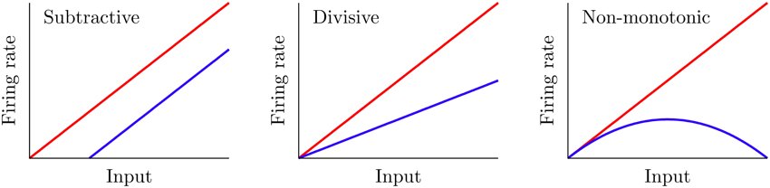
Figure 1. Three different gain control effects commonly observed in real neural systems. The red curve corresponds to the f-I curve before the gain modulation, and the blue curve shows it after the modulation. Subtractive gain control implies a shift of the original f-I curve, while divisive control leads to a change in slope. Non-monotonic gain control usually reflects more sophisticated input–output properties of neurons and synapses.

Mechanisms providing the other two types of gain control shown in Figure 1 have been more elusive. Divisive gain control is often assumed in rate models of neurons and neural populations (Carandini and Heeger, 1994; Chance and Abbott, 2000). However, biophysical mechanisms for such a gain modulation have been hard to identify (Holt and Koch, 1997; Doiron et al., 2001; Chance et al., 2002). On the other hand, non-monotonic gain control has been reported to be induced by short-term depression (de la Rocha and Parga, 2005; Lewis et al., 2007). However, general biophysical mechanisms which cover all these gain control strategies have been difficult to identify and characterize up to date.

In this work, we present a computational model of a neural circuit which is able to display these three types of gain control (subtractive, divisive, and non-monotonic). We consider a generic neural circuit in which neurons receive a given stimulus both directly, i.e., from sensory receptors, and indirectly, via inhibitory interneurons driven by the same stimulus (a pathway referred here as feedforward inhibition, but that is also known in this context as open-loop feedback Litwin-Kumar et al., 2012). Our results, both numerical and analytical, show that these neurons can exhibit the three different types of gain control described above (and shown in Figure 1). The particular type of gain control exhibited by the system depends on (1) the noise level present on neurons and (2) the strength of the negative input provided by the inhibitory neurons, which may be easily modulated in real circuits via long-term synaptic plasticity and therefore provides a highly versatile gain control mechanism. We also carefully analyze the conditions under which the f-I curve of the neural system becomes non-monotonic.

In addition to these results, we also study the above gain control mechanism in the case in which the feedforward inhibition introduces a temporal delay in the signal transmission (reflecting the presence of finite propagation times in the real brain). The existence of such a delay increases the variability of the effective current arriving to the neurons, which in turn leads to a linearization of the f-I curves. The gain control induced by feedforward inhibition is also present in this more realistic scenario. Finally, we use our model to explain the divisive gain control observed in vivo in the superficial pyramidal (SP) neurons of the electrosensory lateral-line lobe (ELL), a cerebellum-like structure of the weakly electric fish Apteronotus leptorhynchus (Bastian, 1986b; see also Figure 2A).

FIGURE 2

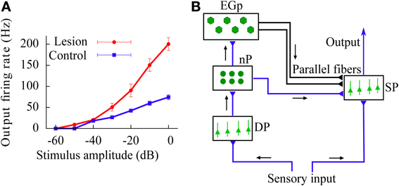
Figure 2. (A) In vivo experimental recording of the firing rate (relative to baseline activity) of SP neurons in the ELL of the weakly electric fish, as a function of the stimulus intensity. Data from control fish is compared with data from fish for which synapses providing the feedforward inhibition via the cerebellar parallel fibers have been removed (lesion). This implies that the effect caused by the parallel fibers is mainly a divisive gain control. Data taken from Bastian (1986b). (B) Scheme of the neural circuit considered in our study. Black arrows show the direction of the input transmission. Parallel fibers are represented by the black lines drawn from the EGp to the SP population. Note that both SP and DP cells receive the sensory input.

2. Materials and Methods

A simplified scheme of the cerebellum-like circuit that we consider in this study is shown in Figure 2B. This circuit resembles the electrosensory lateral-line lobe (ELL), a primary sensory area in the brain of the weakly electric fish Apteronotus leptorhynchus (Maler et al., 1991), although our results can be easily generalized to any circuit in the brain presenting a degree of feedforward inhibition comparable to the one present in the circuit of Figure 2B.

Briefly, sensory inputs coming from electroreceptors arrive to two different pools of neurons: the superficial pyramidal (SP) and the deep pyramidal (DP) neurons (Maler, 2007). Both populations are mainly feedforward, and neurons within a population do not connect between themselves (i.e., no recurrent connectivity). From the population of DP neurons, the stimulus is transmitted to the nucleus praeminentialis (nP) and then to a population of granule cells called the eminentia granularis (EGp). A subset of neurons in the nP directly connects to SP cells and provides an inhibitory feedforward signal. Granule cells of the EGp transmit the signal they receive from a subgroup of nP cells to the SP cells via a massive set of parallel fibers (Berman and Maler, 1999). Apart from a direct excitatory synaptic connection with SP cells, the parallel fibers also synapse onto inhibitory interneurons which then project onto the soma and/or apical dendrites of SP cells and strongly inhibit them. As a consequence of this strong inhibition (or, more precisely, disynaptic inhibition), the overall contribution of parallel fibers to SP neurons is mainly inhibitory (Bastian, 1986b). Note that another subset of nP neurons is excitatory and connects directly to the SP cells as well as disynaptically through inhibitory interneurons. A compelling option is to amalgamate the latter pathway with the other one going directly from the nP to the SP cells. We shall make no further reference to this third pathway. The pathway followed by the sensory stimulus going from DP neurons to SP neurons via the nP and the EGp is called open-loop feedback, or feedforward inhibition (note that both populations receive the stimuli, and thus lie at the same processing stage, however, DP cells send signals to SP cells but do not receive them back). Finally, neurons in the SP population project onto higher areas of the brain.

We consider a population of N deep pyramidal (DP) neurons receiving sensory input from electroreceptors. The membrane potential V^D_i(t) of the DP neuron i follows a simple leaky integrate-and-fire (LIF) dynamics,

$\begin{array}{cc}{\tau }_m\frac{d{V}_i^D(t)}{dt}=-V_i^D(t)+\mu +\sqrt{{\tau }_m}\sigma {\xi }_i^D(t),& (1)\end{array}$

where τ_m is the membrane time constant, μ is the sensory input (that we consider constant for simplicity), and ξ^D_i(t) is a Gaussian white noise of zero mean and delta-type autocorrelation 〈ξ^D_i(t)ξ^D_j(t + τ)〉 = δ_ijδ(τ), with δ_ij and δ(t) being the Kronecker and Dirac delta, respectively. This noise term was included in the model to reflect the intrinsic stochasticity of the deep neurons (Bastian and Nguyenkim, 2001). The factor σ reflects the noise intensity of this stochastic term.

Following the typical dynamics of the LIF model, when the membrane potential reaches a certain threshold V_th, an action potential is generated by the neuron and the membrane potential is reset to V_r, and remains there for a refractory period τ_r.

In the real neural circuit, the population of DP neurons projects onto the nP, then some nP cells project directly onto SP cells while others connect with the EGp, whose granule cells make synaptic contact with the SP neurons both directly and through disynaptic inhibition. In our model, we simplify these intricate feedforward connections by assuming that the activity of the DP population ultimately drives the dynamics of the SP cells, so that the input that a SP neuron receives from the feedforward inhibition pathway is given by

$\begin{array}{cc}f(t)={\tau }_{m}G\frac{1}{N}{\displaystyle \sum _{i=1}^N{\displaystyle \sum _{t_{i,k}}s}}\left(t-t_{i,k}\right).& (2)\end{array}$

Here, the first sum runs over all DP neurons, and the second sum runs over the spike times of each presynaptic DP neuron (i.e., t_i,k is the k-th spike time from the i-th presynaptic neuron). The factor G/N may be identified as the effective strength of synapses onto the SP cells. Since the net polarity of the DP to SP feedforward pathway seems mainly inhibitory (Bastian, 1986b; Doiron et al., 2003), we assume G ≤ 0.

The synaptic filter function, s(τ), describes the effect of a given presynaptic spike on the postsynaptic potential, and it is given by a delayed alpha function

$\begin{array}{cc}s\left(\tau \right)=\left(\frac{\tau -{\tau }_d}{{\tau }_s^2}\right)e^{-\frac{\tau -{\tau }_d}{{\tau }_s}}\Theta \left(\tau -{\tau }_d\right),& (3)\end{array}$

where τ_s is the synaptic transmission time scale, τ_d is a temporal delay, and Θ(x) is the Heaviside step function (i.e., Θ(x) = 1 if x > 0, and Θ(x) = 0 otherwise). Note that s(τ) is normalized so that integration over a large enough time window yields unity.

Equation (2) can also be written by using a convolution of the population average for the DP cells and the synaptic filter. The population average is

$\begin{array}{cc}{Y}^D(t)=\frac{1}{N}{\displaystyle \sum _{i=1}^N{y}_i^D}(t),& (4)\end{array}$

where y^D_i(t) = ∑_ti,k δ(t − t_i,k) is the spike train of DP neuron i. Hence,

$\begin{array}{cc}f(t)={\tau }_{m}G\left(s\ast Y^D\right)(t),& (5)\end{array}$

where (a ∗ b)(t) is the convolution of functions a(t) and b(t).

Since all SP neurons will receive, on average, the same input from sensory receptors and from the feedforward inhibitory pathway, we will consider the response of a typical SP cell, and the output statistics will be valid for all the other SP neurons. The membrane potential V^S(t) of a typical SP neuron is described, as in the case of DP neurons, by a simple leaky integrate-and-fire (LIF) dynamics,

$\begin{array}{cc}{\tau }_m\frac{d{V}^S(t)}{dt}=-V^S(t)+\mu +f(t)+\sqrt{{\tau }_m}\sigma {\xi }^S(t),& (6)\end{array}$

where, as for the DP neurons, μ is the sensory input and the last term considers the intrinsic stochasticity of the neuron (with ξ^S(t) being a Gaussian white noise of zero mean and delta-type autocorrelation). The term f(t) is the input coming from the DP cells and is already known. Again, when the membrane potential reaches the threshold V_th, a spike is generated and V^S(t) is reset to V_r during a period τ_r.

Unless specified otherwise, we choose the following values for the time constants: τ_m = 10 ms, τ_r = 1 ms, τ_s = 5 ms, and τ_d = 10 ms. For parameters related to the membrane potential we consider, without loss of generality, dimensionless units. We set V_th = 1 and V_r = 0, and therefore μ, σ, and G will be in “resting-to-threshold” units. For simulations, we used a DP population of N = 500 neurons unless another size is specified.

3. Results

In the following sections, we will analyze the gain control performed by the DP population on the SP neuron. Even though the gain is properly defined as the derivative of a f-I curve, we shall present f-I curves only since these are the ones usually obtained experimentally—and therefore conclusions arising from the analysis of these curves would naturally translate into results for the derivative of f-I curves. We will compare the f-I curve of a SP cell with and without the feedforward modulation, for different parameter regimes. From Equation (5), setting G = 0 makes the feedforward signal f(t) vanish. But with G = 0, the DP and SP neurons share the same f-I curve since they share the same properties (compare Equation 6 with f(t) = 0 and Equation 1). Hence, the gain control can be fully understood by comparing the SP cell's f-I curve with that of a DP neuron. A gain control will be called subtractive when there is a noticeable shift along the input (i.e., μ) axis in the SP f-I curve with respect to the DP f-I curve. Divisive gain control occurs when the slope (derivative) of the SP f-I curve is mainly scaled by a constant factor with respect to that of the DP population. Finally, a non-monotonic gain control involves the presence of a maximum in the SP f-I curve, so that the scaling factor connecting the slopes of the SP and DP f-I curves changes sign with the input (see Figure 1).

3.1. Subtractive Gain Control

We start our analysis by considering the limit case in which neurons in our system are deterministic (i.e., σ = 0). In this case, the mean firing rate of the DP neurons may be easily obtained by solving Equation (1) for a given neuron. Since the input is the same for all DP neurons, their firing rate will also be the same. One obtains (Tuckwell, 1988)

$\begin{array}{cc}{r}_D={\left[{\tau }_r+{\tau }_m\log \left(\frac{V_r-\mu }{V_{th}-\mu }\right)\right]}^{-1}\Theta \left(\mu -V_{th}\right).& (7)\end{array}$

For convenience, we define the effective bias to the SP cell as the sum of the sensory input plus the feedfoward inhibitory contribution, i.e., μ_eff = μ + f(t). In the diffusion limit (Brunel, 2000), and ignoring fluctuation terms, the effective bias can be written as

$\begin{array}{cc}{\mu }_{\text{eff}}=\mu +{\tau }_{m}G{r}_D.& (8)\end{array}$

In the case of a deterministic system, it takes the form

$\begin{array}{cc}{\mu }_{\text{eff}}=\mu +\frac{{\tau }_{m}G\Theta \left(\mu -V_{th}\right)}{{\tau }_r+{\tau }_m\log \left(\frac{V_r-\mu }{V_{th}-\mu }\right)}.& (9)\end{array}$

Finally, the expression for the SP firing rate is given by

$\begin{array}{cc}{r}_S={\left[{\tau }_r+{\tau }_m\log \left(\frac{V_r-{\mu }_{\text{eff}}}{V_{th}-{\mu }_{\text{eff}}}\right)\right]}^{-1}\Theta \left({\mu }_{\text{eff}}-V_{th}\right).& (10)\end{array}$

The dependence of the effective bias on the sensory input, given by Equation (9), is depicted in Figure 3A. By careful inspection of this figure, one can see that the effective bias increases linearly with μ until μ = V_th. Beyond that point, DP cells start firing and the effective bias starts decreasing, therefore frustrating the firing of the SP cells.

FIGURE 3

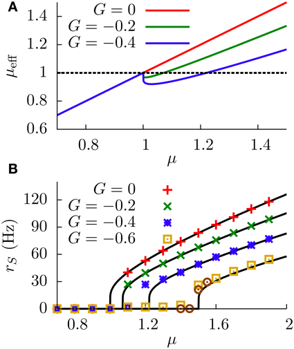
Figure 3. (A) Effective bias entering the SP neuron as a function of the sensory input μ, for the deterministic case (σ = 0). Red line (G = 0) indicates the effective bias for the case in which no feedforward inhibition is considered. (B) Response of the SP neuron to sensory input (i.e., the f-I curve of the SP cell), for the deterministic case. Numerical simulations of a network of N = 100 DP neurons (symbols) show a very good agreement with our theoretical estimations (lines). Circles denote the G = −0.6 case for a network of N = 500 DP neurons, indicating that the small discrepancies between simulations and theory in the firing onset are due to finite-size effects of the simulation.

More precisely, the SP cells will start to fire as soon as μ_eff = μ + τ_mGr_D(μ) becomes greater than V_th. Since we have μ_eff < μ for G < 0, the onsets will occur at different μ values for SP and DP cells, leading to a shift of the gain along the μ axis. This shift becomes evident when we consider the divergences of the SP and DP gains at the firing onsets (the divergences are caused by the derivative of the Heaviside functions appearing in Equations 7, 10). For G < 0, the divergence of the derivative of r_S is shifted to the right on the μ axis with respect to the divergence of the derivative of r_D. Such a shift of the sharp SP firing onset (with respect to the DP firing onset) constitutes a subtractive effect. In addition, for large enough values of μ, the denominator in the second term of the r.h.s. of Equation (9) tends to τ_r, and the effective bias becomes then μ_eff ≃ μ + Gτ_m/τ_r, leading again to a shift of the SP f-I curve for G < 0. It is worth noting that, due to the ratio of time scales τ_m/τ_r ~ 10 obtained for realistic values of the parameters, μ_eff will be significantly smaller than μ even for moderate values of G, which means that SP cells would saturate much later than DP cells along the μ axis.

Based on the above reasoning, one should therefore expect to observe a subtractive effect of the feedforward inhibition on the f-I curve of the SP neuron at zero noise. This is indeed what we observe in Figure 3B, where the results of numerical simulations of the model for σ = 0 show a very good agreement with our theoretical expression given by Equation (10). We can observe that the displacement of the firing onset depends on G as theoretically predicted, with more negative values of G leading to larger shifts of the onset of firing. Therefore, the modulation of the strength G leads to a subtractive gain control in the f-I curve of the deterministic (σ = 0) system.

3.2. Divisive Gain Control

After analyzing the deterministic case, we can now study the more general case in which neurons in the circuit present some level of stochasticity (i.e., σ > 0) in their dynamics. Such a stochasticity may be due, for instance, to the noisy dynamics of ion channels (White et al., 2000), or to synaptic bombardment from other surrounding neurons (Hô and Destexhe, 2000), for instance (see also Longtin, 2013 for a review).

For the stochastic case σ > 0, the mean firing rate of the DP neurons may be obtained by solving Equation (1), and it is given by (Tuckwell, 1989)

$\begin{array}{cc}{r}_D={\left[{\tau }_r+{\tau }_m{\displaystyle {\int }_{z_r^D}^{z_{th}^D}\sqrt{\pi }}{e}^{z^2}\left(1+\text{erf}(z)\right)dz\right]}^{-1},& (11)\end{array}$

where $z_{th}^D\equiv \frac{V_{th}-\mu }{\sigma }$, $z_r^D\equiv \frac{V_r-\mu }{\sigma }$, and erf(z) is the error function. The effective bias is again μ_eff = μ + τ_mGr_D, although the explicit form is more complex now. Finally, we can write the mean firing rate of SP neurons as

$\begin{array}{cc}{r}_S={\left[{\tau }_r+{\tau }_m{\displaystyle {\int }_{z_r^S}^{z_{th}^S}\sqrt{\pi }}{e}^{z^2}\left(1+\text{erf}(z)\right)dz\right]}^{-1},& (12)\end{array}$

where $z_{th}^S\equiv \frac{V_{th}-{\mu }_{\text{eff}}}{\sigma }$ and $z_r^S\equiv \frac{V_r-{\mu }_{\text{eff}}}{\sigma }$.

The main effect of the addition of noise to the DP neuron model is the appearance of a smooth linearization around the onset of the f-I curve for these neurons (Doiron et al., 2001). This is due to noise-induced firing, which is especially important when the neuron is slightly below the firing threshold.

As a consequence of this linearization, the effective bias μ_eff may be approximately described, for values of μ close to the DP firing onset, as

$\begin{array}{cc}{\mu }_{\text{eff}}=\mu +{\tau }_{m}G{r}_D\simeq \mu +{\tau }_{m}G\left(C_1\mu +C_2\right),& (13)\end{array}$

where C₁ and C₂ are constants, with C₁ » C₂ for realistic values of the parameters. The effective bias, therefore, would be approximately linear, with a slope that depends on G. Such a linear dependence is shown in Figure 4A, where we can see that μ_eff is indeed well approximated by a linear relationship with μ, and that the slope depends on G. In particular, as G goes to more negative values the slope of the μ_eff − μ relationship decreases. We will restrict ourselves here to the case of G having relatively small absolute values, so that μ_eff will be an increasing function of μ in all cases. Large negative values of G, which could compromise this tendency, will be addressed in the next section.

FIGURE 4

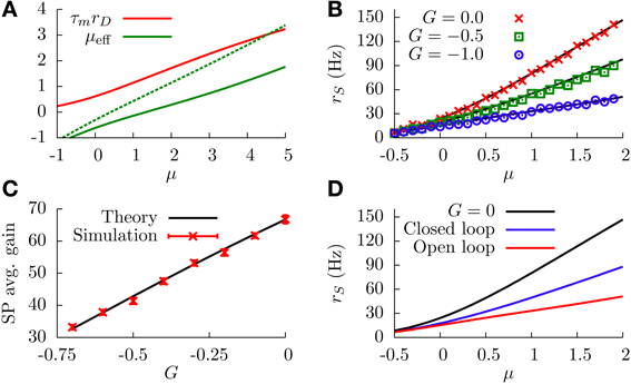
Figure 4. (A) DP firing rate (red line) and effective bias (solid green line) as a function of the sensory input μ. One can see that both curves can be considered as approximately linear with μ (this is valid as long as |G| is not very large). Parameters are $\sigma =\sqrt{3}$, G = −1. The green dotted curve is the same as the solid green line, but for G = −0.5. (B) SP firing rate as a function of the sensory input, for different values of G and σ = 1. The divisive gain control occurs as G takes larger negative values. (C) Average gain of the SP f-I curve as a function of G, for σ = 1. The average gain is obtained by fitting the f-I curve with a linear function over a range of μ values for which the curve is approximately linear. The displayed results differ by the origin of the f-I curves used. For the solid black line, the rates are computed from the analytical formula (Equation 12). For the red symbols, the f-I curves are extracted from simulations of network. The error bars come from the fitting procedure, and serve to illustrate how linear the f-I curves are for the chosen μ ranges. (D) Comparison between the divisive gain control in our model (open-loop feedback) and the one studied in Sutherland et al. (2009) (closed-loop feedback), for σ = 1. As the panel shows, the open-loop feedback mechanism studied here provides a stronger divisive effect than the one studied by Sutherland et al. for the same feedback strength and conditions. Both the open-loop and closed-loop cases correspond to the same strength, G = −1. For all panels, solid or dotted lines come from theoretical (analytical) expressions, whereas symbols come from simulations.

Interestingly, since the f-I curve of an isolated SP neuron is also linearized by the presence of stochasticity, the above approximation can be applied again: the multiplicative effect that G has on the slope of μ_eff will also affect the slope of the SP f-I curve in the same way. Indeed, by comparison of Equations (11, 12), we can see that the response of a SP cell to μ_eff is identical to the response of a DP cell to μ, so we can assume the same linear dependence r_S ≃ C₁μ_eff + C₂ and arrive at the following divisive relationship

$\begin{array}{cc}{r}_S=\left(1+C_1{\tau }_m G\right)r_D.& (14)\end{array}$

This relationship also holds, in an approximate way, when one solves Equation (12) analytically, without considering any explicit linearization of the firing rates. This is shown in Figure 4B, where one can observe that increasing the strength of the feedforward inhibition has a divisive effect on the f-I curve of the SP neuron, as predicted. The figure also shows the good agreement between numerical simulations of the model and the theoretical expression, given by Equation (12). Figure 4C shows more clearly the relation between G and the SP gain, and we observe that larger negative values of G produce a smaller slope on the SP f-I curve. Consequently, the modulation of the feedforward inhibitory strength (in the range of small |G|) provides a divisive gain control to the system when stochasticity is considered.

In the mechanistic description presented above, the divisive gain modulation strongly depends on the fact that DP neurons drive the response of SP neurons without any restrictions (such as feedback from other cells to the DP neurons). This approach differs from previous attempts to explain the divisive gain control found in vivo (Bastian, 1986b), such as the one presented in Sutherland et al. (2009). In this previous approach, Sutherland et al. considered a unique population of ELL pyramidal cells, without distinguishing between DP and SP neurons. The system was then assumed to display a closed-loop feedback circuit, in which the population of pyramidal neurons projected their output to a feedback kernel, which in turn inhibited the activity of the population. Because the negative feedback was affecting all neurons in this case, a high firing rate would be prevented by the closed-loop inhibition. In the approach we present here, on the other hand, DP neurons (which drive the gain control of SP cells) do not receive inhibitory feedback, and therefore they are able to raise their firing rate higher and produce a stronger and more effective modulation of the SP firing rate than in the closed-loop scenario. This can be seen in Figure 4D, where our open-loop model is compared with a closed-loop version of the same model for the same values of the parameters (the case G = 0 is also shown for comparison). In the closed-loop model, the firing rate of the unique pyramidal cell population ν is given by

$\begin{array}{cc}\nu ={\left[{\tau }_r+{\tau }_m{\displaystyle {\int }_{z_r}^{z_{th}}\sqrt{\pi }}{e}^{z^2}\left(1+\text{erf}(z)\right)dz\right]}^{-1},& (15)\end{array}$

where $z_{th}=\frac{V_{th}-\mu -{\tau }_{m}G\nu }{\sigma }$ and $z_r=\frac{V_r-\mu -{\tau }_{m}G\nu }{\sigma }$. It is worth noting that both z_th and z_r depend on the population firing rate ν, and therefore Equation (15) has to be solved recursively. As Figure 4D shows, the open-loop model proposed here allows for a stronger modulation than the closed-loop model for the same parameter values and, in particular, for the same value of G in both cases.

3.3. Non-Monotonic Gain Control

In the previous section, we assumed small absolute values of G to simplify our treatment. This allowed us to understand, from a qualitative point of view, the origin of the divisive gain control in our feedforward inhibitory pathway system, and our findings were supported by both our numerical simulations and our theoretical description. However, these results could be different for larger values of G, as a strong feedforward inhibition driven by sensory input could overcome the excitatory effects of this same sensory input on SP cells. If that were the case, μ_eff would no longer increase with μ (or, at least, not for all values of μ), and the effect of G on the f-I curve might change. In order to explore such a possibility, we need to consider a more careful analysis of the stochastic case (i.e., σ > 0) for large values of G.

We start by identifying potential extrema in the f-I curve of the SP neuron, which would be an expected effect of feedforward inhibition overcoming excitation in SP cells for a given value of μ. Since the SP firing rate is a monotonically increasing function of μ_eff (see Equation 12), finding the extrema of the effective bias as a function of μ would be equivalent to finding the extrema of the f-I curve for SP cells. The condition for extrema of the effective bias μ_eff = μ + τ_mGr_D can be obtained from $\frac{d{\mu }_{\text{eff}}}{d\mu }=0$, and it gives

$\begin{array}{cc}\frac{d{r}_D}{d\mu }=-\frac{1}{{\tau }_{m}G},& (16)\end{array}$

or, in a more explicit form,

$\begin{array}{cc}\sigma +\sqrt{\pi }{\tau }_m^{2}G{r}_D^2\left[e^{z_{th}^2}\left(1+\text{erf}\left(z_{th}\right)\right)-e^{z_r^2}\left(1+\text{erf}(z_r)\right)\right]=0.& (17)\end{array}$

We will consider the condition of extrema in its simplified version (i.e., Equation 16) for clarity. The relationship r_D versus μ, given by Equation (11), takes a sigmoidal-like shape: r_D tends to zero for large negative μ, and to 1/τ_r for large positive μ. The maximum slope reached by r_D (which we will denote as γ) would be located somewhere between these two limits. Therefore, $\frac{d{r}_D}{d\mu }$ would follow approximately a bell shape: it is zero at both ends of the μ axis, and it has a maximum (of value γ) for a moderate value of μ.

With this information, and together with Equation (16), it is easy to see that extrema will exist only when $\gamma >\frac{1}{{\tau }_m\left|G\right|}$, which typically occurs for large enough absolute values of the feedforward inhibitory strength. In this case, we will have two extrema (since $\frac{d{r}_D}{d\mu }$ is bell-shaped and will cross the constant level $\frac{1}{{\tau }_m \left|G\right|}$ twice). Figure 5A shows $\frac{d{r}_D}{d\mu }$ as a function of μ, in a situation in which the two extrema exist.

FIGURE 5

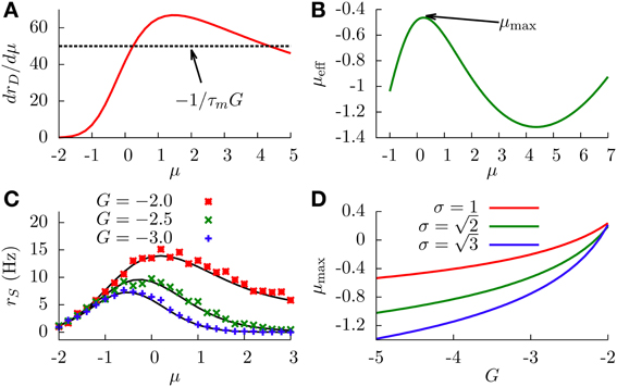
Figure 5. (A) Graphical representation of the condition for the existence of extrema (Equation 16). We can see that solutions for this equation exist only when γ (the peak value of the curve) is larger that $\frac{1}{{\tau }_m\left|G\right|}$ (dashed line). Parameters are σ = 1 and G = −2. (B) Effective bias as a function of μ, showing the existence of a maximum and a minimum. Parameters are σ = 1 and G = −2. (C) SP firing rate as a function of the input μ, for different values of G, displaying non-monotonic gain control. We chose $\sigma =\sqrt{2}$. (D) Position of the SP firing rate peak (shown in panel C) as a function of G, for different values of σ. In all panels, solid lines come from theoretical (analytical) expressions, whereas symbols come from simulations.

The concrete shape of the effective bias with μ is shown in Figure 5B. The two extrema correspond to a maximum (at small μ) and a minimum (at larger μ). This yields a bell-shape dependence of the effective bias on μ (at low values), followed by an increase with μ (for high values). The cause for this behavior is the following: at very small values of μ, the firing rate of the DP neurons is not high enough, and the main contribution to the effective bias is the sensory stimulus μ, with the feedforward inhibition playing a minor role. As μ makes the DP firing rate increase, the feedforward inhibition term becomes dominant (since G is negative and large) and the effective bias starts to decrease, completing the bell-shape profile observed in Figure 5B. After that, and for very large values of μ, the DP firing rate approaches its saturation value 1/τ_r. At this point the sensory stimulus μ becomes the dominant term and μ_eff begins to rise again. It is worth noting that this second rising of μ_eff occurs at input levels where the firing rate of DP neurons saturates, and such sensory input levels are beyond the range in which biologically relevant information can be linearly processed in the system, according to electroreceptor input–output characteristics (Gussin et al., 2007). The attainment of the maximum rate, however, occurs for biologically sound biases, as exemplified in Figure 5C.

Since the firing rate of SP cells monotonically increases with the effective bias, the maximum and minimum found in μ_eff are also observed for the SP firing rate, as shown in Figure 5C. This implies that, for a stochastic system, enhancing the negative feedforward strength may drive the system from a divisive to a non-monotonic gain control regime. The figure also shows that the location and height of the peak of the SP firing rate is also modulated by G. This is to be expected, since the stronger the inhibition, the sooner the DP firing rate will start decreasing the effective bias. Large negative values of G will shift the location of the SP firing rate peak toward lower values of μ, as can be observed in Figure 5C and, with more detail, in Figure 5D. The level of stochasticity has also an impact on the position of the peak: larger values of σ will increase the overall firing rate of DP neurons, and the resulting increment in the feedforward inhibition will shift the peak toward even lower values of μ, as Figure 5D also shows.

Our neural circuit, therefore, is able to display three different regimes, corresponding to subtractive, divisive, and non-monotonic gain control. As the theory and numerical simulations show, both the level of stochasticity σ and the feedforward strength G play an important role in the behavior of the system. Figure 6 shows a phase diagram of the system as a function of these two parameters. The subtractive gain control is observed only for deterministic systems (σ = 0), since the introduction of some level of noise would smooth the DP firing onset and we would go into other regimes. For σ > 0 the system can be in the divisive or non-monotonic regime, depending on the value of G. As discussed in the previous section, small absolute values of G would linearize the DP rate, effective bias and SP rate with respect to μ, leading to the appearance of divisive gain control. For large negative G, the feedforward inhibition can eventually overcome the input μ to the SP neuron and the circuit will display non-monotonic gain control. The critical line separating the divisive and non-monotonic regimes is given by

$\begin{array}{cc}\gamma =\frac{1}{{\tau }_m\left|G\right|}.& (18)\end{array}$

To obtain the critical line in Figure 6, we varied G—from within the divisive region—for each value of σ until the condition for extrema (Equation 17) at finite values of μ was first met (and actualizing Equation 18).

FIGURE 6

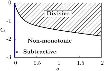
Figure 6. Phase diagram of the neural system studied. The subtractive gain control regime corresponds to the σ = 0 axis, and the critical line separating the divisive and the non-monotonic gain control regimes is given by Equation (18).

We emphasize that, in order to get a non-monotonicity in the SP firing rate, the derivative of the effective bias must vanish for a certain μ value, and the SP cell must have a non-zero firing rate around that value. Because of these two conditions, a non-monotonic behavior cannot be obtained for zero noise. Indeed, in the absence of noise, the DP firing rate is not differentiable at the μ value for which the maximum should occur, and furthermore the SP firing rate would be zero for that μ value.

We simplified the above analysis of the system by assuming that the SP and DP cells share the same properties, namely the same bias (μ) and the same level of noise (σ). We argue that this analysis can be extended to more general contexts. In real systems, neural attributes are not uniform. For instance, in the cortex, inhibitory interneurons fire irregularly in response to constant inputs in vitro (Stiefel et al., 2013), whereas pyramidal neurons are relatively regular (Mainen and Sejnowski, 1995). In the ELL, even though both the SP and the DP cells receive a common external input, they do not possess the same variability (Bastian and Nguyenkim, 2001), which may translate into different biases and noise intensities. Furthermore, even a weak neuron-to-neuron variability among the neural populations could induce non-trivial effects in information processing (Mejias and Longtin, 2012; Nicola et al., 2013). Above, we amalgamated the intrinsic bias and the applied current (I_app, say) under the umbrella variable μ. To accommodate different neural properties, we could use two separate intrinsic biases (μ_S and μ_D) and noise intensities (σ_S and σ_D), and study the SP firing rate as a function of I_app. This could produce slightly different results than above. As an example, for the noiseless case (σ_S = σ_D = 0), the SP cells could start to fire before the DP neurons—provided that μ_S is large enough—, stay active for a limited range of I_app values, become silent when the DP cells attain a sufficient rate, and then fire again for higher I_app. This would constitute a mixed regime showing both non-monotonic and subtractive gain controls. Note that this mixed regime is also observable for uniform neural properties when the noise is low. In the latter case, the isolated blob of non-zero firing rate is due to noise.

3.4. Time-Dependent Stimuli and Synaptic Delays

Real neural systems deal with time-dependent stimuli. In sensory networks, neurons are responsible for encoding the temporal features of information coming from the environment. When dealing with time-dependent signals, a number of factors have to be considered in addition to the ones included up to now in our study. For instance, the existence of temporal delays in the transmission of information, due to the finite transmission speed of action potentials along the axons, becomes important. In the particular case of the ELL, signals from the DP cells have to travel through different neural populations before arriving to SP cells. Traveling such a distance causes a temporal delay in the transmission that, in some cases, may reach tens of milliseconds (Maler et al., 1991; Bol et al., 2011). Although this temporal delay did not have an effect in our previous results, with μ being constant in time (data not shown), it might have a significant impact in more realistic situations, when the sensory input presents temporal fluctuations and some level of autocorrelation. Different synaptic filter functions s(τ) might have an effect in these realistic situations as well.

To test our model for these conditions we use, as sensory input, a time-varying quantity $\widehat{\mu }(t)$ of the form

$\begin{array}{cc}\widehat{\mu }(t)=\mu +\zeta (t),& (19)\end{array}$

where μ is the constant bias, and ζ(t) is a gaussian low-pass filtered noise of zero mean and standard deviation σ_c. This noise term is generated using a Butterworth fourth-order digital filter with cut-off frequency of 100 Hz. In the following, to explore the behavior of our model for other synaptic filter functions, we consider a delta-type synaptic function s(τ) = δ(τ − τ_d).

When the temporal delay τ_d is set to zero, the main effect of considering this slowly fluctuating input is a slight increase in the SP firing rate along the f-I curve, as Figure 7A shows. The black line in the figure shows the f-I curve for σ_c = 0, and the red line shows the same f-I curve for σ_c = 1. This firing rate increase is simply due to the presence of the extra fluctuating term ζ(t).

FIGURE 7

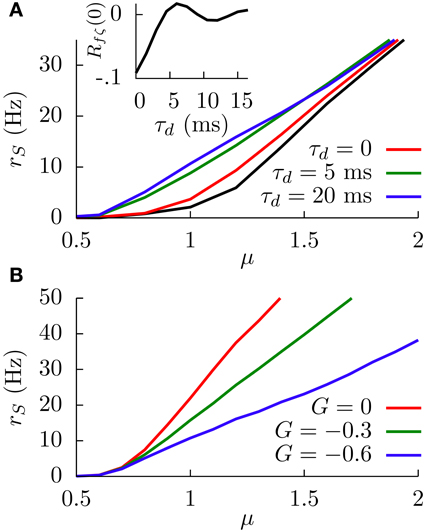
Figure 7. (A) Simulation results of the effect of the temporal delay on the f-I curve of the system at G = −0.6. The black line corresponds to the case in which the sensory input is just a constant bias and only the white noise is present. For other curves, the fluctuating term ζ(t) is also present, and the effect of varying τ_d is shown. Inset: Theoretical dependence of the covariance of f(t) and ζ(t) on the temporal delay. (B) Simulation results of the SP firing rate versus constant bias for different values of G, a white noise term, and a slow fluctuating term ζ(t), for a temporal delay τ_d = 20 ms. In both panels, we have σ = 0.1, σ_c = 0.3, and τ_m = 15 ms.

The figure also shows, interestingly, that considering temporal delays τ_d larger than zero leads to a significant increment in the SP firing rate, especially around the firing onset. To understand this phenomenon, it is useful to consider a slow (with respect to τ_m) positive fluctuation in $\widehat{\mu }(t)$, arriving at DP and SP neurons simultaneously. If the temporal delay τ_d of our circuit from DP cells to SP cells is zero, the transient increment in the sensory input received by the SP neuron will be compensated almost simultaneously (apart from the response time) by the transient increment of the DP firing rate, which will have an inhibitory effect on the SP neuron since G < 0. The effective bias received by the SP neuron, therefore, will be mainly unaffected by such a fluctuation.

In the presence of some level of temporal delay, however, this “compensation” from the DP cells may arrive late, maybe once the transient increment in SP firing due to the fluctuation is over. Even more, this late compensation from DP cells could cause a transient decrement in the effective bias that the SP neuron receives. As a consequence, the effective bias arriving at the SP cells will be highly fluctuating, and these input fluctuations will cause an increment in the SP firing rate. This novel variability-increasing effect would be especially important around the SP firing onset, and our simulation results confirm this point (Figure 7A). The effect of the temporal delay on the level of fluctuations in the effective bias can also be mathematically derived (see Appendix). Indeed, our calculations show (inset in Figure 7A) that the covariance of f(t) and ζ(t), and therefore the fluctuations of the effective bias, increases from negative values toward zero with the temporal delay τ_d (with some minor oscillatory component), supporting these findings on the delay-induced effects on SP firing rate. Time-dependent stimuli would also induce correlations between DP and SP cells, which would depend on the temporal delays along with a number of other factors (Ostojic et al., 2009).

In Figure 7B, one can see an example of the divisive gain control for this more realistic situation with delay. In this case, the sensory input has a fluctuating part ζ(t) and a temporal delay of 20 ms. The behavior of the system is qualitatively similar to the one observed previously (i.e., large negative values of G induce a divisive effect on the gain of the f-I curve). The non-monotonic behavior also holds for this more realistic model (data not shown).

In our treatment of the effect of delay on the f-I curve, we assumed that the feedforward inhibitory strength G is a constant. That is, G had the same magnitude for all frequencies contained in the signal. This may not be the case for real systems. For instance, in the weakly electric fish, the EGp parallel fibers are known to be inactive when sinusoidal signals of higher frequency than about 20 Hz are applied to the network (Bol et al., 2011). On the other hand, the direct inhibition coming from the nP seems to be active for an extended frequency range (Doiron et al., 2004). So, G may generally depend on frequency in a non-trivial way. This fact can easily be included into the result for the covariance of f(t) and ζ(t) appearing in the Appendix, provided that one knows—at least approximately—how G changes with frequency. If, for example, G is zero above a given frequency, then, obviously, signals only containing frequencies above that cutoff should have no effect on the f-I curve.

3.5. Comparison with Experimental Data

We now apply our model to in vivo data showing gain control in SP cells of weakly electric fish (Bastian, 1986b). In Figure 2A, reproduced from Bastian (1986b), the firing rates of SP cells in control fish is compared with those in fish for which the EGp has been lesioned. The result of this procedure is to eliminate the signal coming from the parallel fibers. Bastian's results show that the EGp contribution modulates the f-I curve of SP neurons, producing a divisive gain control. Since this form of gain control has been identified as one of the behaviors displayed by our model, it might be interesting to test whether the model is able to quantitatively explain the experimental data. Here, we shall restrict ourselves to analytical f-I curves (Equation 12) since they have been shown to be in good agreement with those extracted from numerical simulations of Equations (1, 6). The experimental results are given as relative firing rates versus the stimulus intensity in decibels. To apply our model, we first need to convert these relative firing rates to absolute ones and relate the experimental stimuli to our μ.

The stimuli are amplitude modulations (AMs, in mV/cm) of the fish's electric field. In mathematical expressions we shall denote the intensity of these AMs by the symbol E_AM. The zero-decibel reference is E^ref_AM = 2 mV/cm (Bastian, 1986b), so that the number of decibels is given by 20 log₁₀(E_AM/E^ref_AM). Relative firing rates for the lesion and control cases are given by the rates for given AMs from which is subtracted the rate in the spontaneous regime (i.e., when E_AM = 0). More precisely, absolute firing rates are given by

$\begin{array}{cc}{r}_S^{C(L)}\left(E_{\text{AM}}\right)=r_S^{C(L)}(0)+\Delta r_S^{C(L)}\left(E_{\text{AM}}\right),& (20)\end{array}$

where Δr^C(L)_S(E_AM) represents relative firing rates in the control (lesion) case. From Bastian (1986a), it appears that r^C_S(0) − r^L_S(0) ~ 10 Hz, which means that the net effect of the EGp parallel fibers is actually excitatory in the spontaneous regime. On the other hand, it is clear from Figure 2A that the EGp contribution is inhibitory for larger E_AM. Therefore, this contribution changes sign somewhere between 0 and 2 mV/cm. From inspection of Figure 8A, in which absolute firing rates are plotted, this transition occurs for a small AM value (where the lesion and control curves intersect).

FIGURE 8

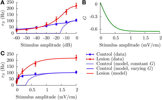
Figure 8. Divisive gain control measured in SP cells in vivo and the theoretical predictions of our model. (A) Absolute firing rates (in contrast to Figure 2A where rate changes relative to baseline were plotted) as a function of the stimulus amplitude in decibels. Experimental absolute rates (symbols) are obtained from the relative rates appearing in Figure 2A by adding the baseline rates for the lesion and control cases (see text for details, especially Equation 20). To simulate the lesion (i.e., absence of parallel fibers) in the model, we set G = 0 (red line). The theoretical control curves (solid and dashed blue lines) differ by the assumptions on G. For the dashed blue line, G = −0.65 for all amplitude modulations; for the solid one, G is given by the curve illustrated in panel (B) (G(E_AM) = G₀ + B/[1 + exp(−κE_AM)], with G₀ = 0.75, B = −1.4, and κ = 5). Panel (C) contains the same information as panel (A), but with a linear scale for the x axis.

We now relate the AMs to our μ. The SP and DP cells receive input from electrosensory afferents, which encode the AMs of the electric field. We consider that μ encompasses an intrinsic bias μ₀ and a simple summation of these afferent inputs. The average input to a ELL pyramidal cell is then

$\begin{array}{cc}\mu ={\mu }_0+{\tau }_m{G}_{\text{aff}}{r}_{\text{aff}}\left(E_{\text{AM}}\right)\equiv {\mu }_0+\gamma \left(E_{\text{AM}}\right),& (21)\end{array}$

where G_aff is the afferent synaptic strength times the number of afferents (compare with Equation 8). The afferents' firing rate, r_aff(E_AM), is a sigmoid taking the form of a Boltzmann function (Benda et al., 2005):

$\begin{array}{cc}{r}_{\text{aff}}\left(E_{\text{AM}}\right)=\frac{r_{\text{max}}}{1+e^{-k\left(E_{\text{AM}}-h\right)}},& (22)\end{array}$

where r_max is the maximum firing rate. The slope of the linear part of this curve is given by r_maxk/4, whereas h is the AM value at which r_aff = r_max/2. Replacing Equation (22) into (21) provides the required relationship between μ and E_AM. We further define the constant A ≡ τ_mG_affr_max.

To fit the data corresponding to a lesioned fish, i.e., which lacks the set of parallel fibers connecting the EGp with the SP cells, we set G = 0. This is not rigorously true since, from Figure 2B, the direct inhibitory signal from the nP could still be active, and hence G should not be strictly zero. However, given the overall large effect that the parallel fibers have on the SP cells' f-I curve (Figure 2A), it seems plausible to neglect the nP component of the total feedforward inhibitory pathway in first approximation. Heuristically, we could write G = G_EGp + G_nP, where G_EGp (respectively G_nP) is the strength of the feedforward inhibition coming from the EGp (respectively nP). Then the effective bias would be expressed as μ_eff = μ_0,S + γ(E_AM) + τ_m(G_EGp + G_nP)r_D, with μ_0,S the AM-independent bias of the SP cell, which is assumed to be different than that of the DP cells. Our approximation consists in setting μ_0,S + τ_mG_nPr_D ≈ μ_0,D ≡ μ₀ and identifying G_EGp with G.

All parameters other than G are assumed identical for the lesion and control cases. These parameters were determined by inspection of the lesion data and by comparison with other studies of the ELL pyramidal neurons (Doiron et al., 2003, 2004; Bol et al., 2011; Mejias et al., 2013). The time constants are τ_m = 6 ms and τ_r = 0.8 ms. The noise intensity σ is set to 0.01. Such a small value is prescribed by the overall aspect of the lesion firing rate when plotted against a linear scale for the AMs (Figure 8C). To model the input μ, we set μ₀ = −0.16, A = 2.31, and k = 3 cm/mV. A range of plausible values for k has been established from an inspection of Figure 6D in Benda et al. (2005). The parameters μ₀ and A are then set in such a way that the theoretical f-I curve for the lesion case adequately fits with the corresponding experimental results. Also, h is set to 0 mV/cm to simplify. From Figure 8A (or C), one sees that the red line (lesion) is a good fit to the experimental curve.

For the control case, making G a constant for the whole range of AMs is incompatible with the experimental results for low AMs. The dotted blue curves in Figures 8A,C illustrate this point. For instance, fixing G = −0.65 makes the theoretical f-I curve agree with the experimental results for large AMs, but it fails to model what happens for smaller AMs. The agreement for large AMs is mainly due to the saturation of the afferents' activity, i.e., μ does not vary appreciably under strong stimulations. Consequently, the divisiveness of the gain control at large amplitudes results from a different mechanism than the one presented up to now in the paper. For small AMs, given the very low noise intensity, a moderately high negative feedforward strength naturally yields a subtractive gain control. To get a divisive gain control for small AMs, we have to take into account the variation of G with the stimulus amplitude E_AM.

As discussed above, the feedforward strength G changes from negative to positive values as E_AM decreases from 2 to 0 mV. The theoretical firing rate for the control case fits with the experimental one for E_AM = 2 mV if we set G = −0.65. It is reasonable to assume that G saturates for large positive and negative AM values. A simple function comprising these characteristics is a sigmoid akin to that given in Equation (22), but with a negative “r_max.” It is displayed in Figure 8B for positive AMs. The solid blue curves in Figures 8A,C show a good agreement between theory and experiment when this function is used. We stress, however, that this function has been determined in a purely ad hoc way to illustrate that a varying G is necessary.

Our simple model is able to explain the divisive gain control obtained in vivo for the SP cells as long as the feedforward strength is allowed to change with the stimulus amplitude. As stated in section 2, the SP cells receive direct excitation and disynaptic inhibition from the parallel fibers. These contributions have different respective weights depending on the stimulus intensity, yielding a variable net feedforward strength (Lewis et al., 2007). Also, SP cells possess receptive fields of the ON center-OFF surround type (Maler, 2007). Center and surround have different activation thresholds (Bastian et al., 2002), so the proportion of inhibition and excitation depends on the intensity of AMs. Such a differential activation might have an impact on phenomena depending on a neuron's activity, namely the synaptic plasticity.

4. Discussion

The modulation of input–output characteristics is a major strategy used by neural systems for the processing and gating of information. Neurons able to change their f-I (firing rate versus input) curve stand as a prominent example of this. While very general mechanisms are known to produce subtractive gain control, mechanisms providing other forms of modulation, such as divisive or non-monotonic gain control (see Figure 1), have been harder to identify (Holt and Koch, 1997; Chance and Abbott, 2000; Doiron et al., 2001; Chance et al., 2002; Longtin et al., 2002; Sutherland et al., 2009). In this work, we presented a biologically plausible mechanism which yields subtractive, divisive and non-monotonic gain control. We analyzed, both with theoretical approaches and numerical simulations, the conditions for which each behavior may appear. The mechanism is based on the interaction between noise and some level of input-driven feedforward inhibition, and constitutes an example of a generic neural strategy which can produce different types of computationally-desirable modulations of f-I curves.

The concrete neural circuit considered in the study is very general: a feedforward neural assembly inhibits target neurons, and both populations receive a common external input. Such a circuit has already been used to study the role of feedforward inhibition in decorrelating neural activity in the somatosensory cortex of rats (Middleton et al., 2012). In the present work, it is used to model the ELL of the weakly electric fish. The feedforward population is composed of so-called deep pyramidal (DP) neurons, whose targets are neurons that inhibit superficial pyramidal (SP) cells. It is the modulation of the SP cells' firing activity that is studied here. However, the simplicity of the network and neuron models suggests that our results could apply to other systems with a similar structure.

As stated before, the f-I behavior of the neural network depends on the level of neural noise and the strength of the feedforward inhibition. In most situations, when neurons present some level of stochasticity, the feedforward inhibitory strength will determine whether the gain control is divisive or non-monotonic. This makes the system highly versatile, since the feedforward inhibitory strength, which can be seen as efficacies of the synaptic connections involved, could be modulated by long-term synaptic plasticity. This might be the case in the ELL of the weakly electric fish, as different types of long-term plasticity have been identified in the parallel fiber synapses with SP neurons in this and other species of electric fish (Han et al., 2000; Harvey-Girard et al., 2010). If that were the case, then as the inhibitory feedforward contribution becomes stronger, the divisive gain control observed experimentally in SP cells would turn into a non-monotonic gain control. Indeed, non-monotonic f-I curves for SP neurons have been recently observed in vitro under direct parallel fiber stimulation (Figure 3C in Lewis et al., 2007), supporting this hypothesis. Further experimental work, however, is needed to adequately test our prediction of non-monotonic gain control emerging for strong feedforward inhibition.

The existence of a non-monotonic gain control regime, as hypothesized by our modeling study and suggested by recent experimental findings (Lewis et al., 2007), would have interesting functional advantages with respect to monotonic relationships. For instance, a non-monotonic dependence in the f-I curve of a neural circuit would allow for having a high gain (i.e., high sensitivity) for low and moderate input levels while ensuring, by decreasing firing rates, that the energy constraints of the circuit are met for large inputs (something that a monotonic f-I curve cannot provide). Interestingly, it has been proposed that the non-monotonic input–output relationship caused by a combination of short-term synaptic depression and facilitation could be important for detection of coincident spikes (Mejias and Torres, 2008) and burst transmission (Izhikevich et al., 2003). Similar features might be present in our system as well, since the non-monotonic input–output profiles that we obtained via feedforward inhibition are similar to those given by short-term synaptic plasticity.

The gain control mechanism presented here holds for more realistic situations, such as when considering a time-dependent sensory stimulus. In the presence of complex input signals, the presence of temporal delays in the systems becomes an important factor, and we have considered it in our study as well. The introduction of a temporal delay in our feedforward inhibitory term revealed a novel effect in the dynamics of the system: as the delay increases, an excitatory input fluctuation arriving to a SP cell from the senses does not coincide in time with its inhibitory counterpart arriving from the inhibitory feedforward pathway. As a consequence, the level of fluctuations arriving at SP cells increases, which in turn increases the SP firing rate, especially near the firing onset. Our theoretical approach is able to explain this effect as well (see Appendix). In spite of these new effects in the dynamics of SP cells, the feedforward-driven gain control remains the same as in the original model, indicating that the mechanism can work as well for time-dependent stimuli.

Finally, we found that the basic model used to obtain the aforementioned gain control regimes is able to describe the divisive gain control observed in vivo in the SP cells of the ELL (Bastian, 1986b) for moderate to large stimuli. For low amplitude stimuli, the control has a significant subtractive component. Once the model is augmented with a feedforward inhibitory strength that depends on stimulus intensity, it exhibits divisive behavior at all amplitudes (i.e., even for low amplitude stimuli). This illustrates the versatility of our model, and shows how it can be modified to depict more subtle gain control phenomena in real systems.

Conflict of Interest Statement

The authors declare that the research was conducted in the absence of any commercial or financial relationships that could be construed as a potential conflict of interest.

Acknowledgments

This work was funded by the Natural Sciences and Engineering Research Council of Canada (NSERC) and in particular its Discovery Accelerator program, the Canadian Institutes for Health Research (CIHR) and the Fonds de Recherche en Sciences Naturelles et Technologies du Québec (FQRNT).

References

Abbott, L. F., Varela, J. A., Sen, K., and Nelson, S. B. (1997). Synaptic depression and cortical gain control. Science 275, 220–224. doi: 10.1126/science.275.5297.221

Pubmed Abstract | Pubmed Full Text | CrossRef Full Text

Alitto, H. J., and Usrey, W. M. (2004). Influence of contrast on orientation and temporal frequency tuning in ferret primary visual cortex. J. Neurophysiol. 91, 2797–2808. doi: 10.1152/jn.00943.2003

Pubmed Abstract | Pubmed Full Text | CrossRef Full Text

Andersen, R., and Mountcastle, V. (1983). The influence of the angle of gaze upon the excitability of the light- sensitive neurons of the posterior parietal cortex. J. Neurosci. 3, 532–548.

Pubmed Abstract | Pubmed Full Text

Bastian, J. (1986a). Gain control in the electrosensory system: a role for the descending projections to the electrosensory lateral line lobe. J. Comp. Physiol. A 158, 505–515. doi: 10.1007/BF00603796

Pubmed Abstract | Pubmed Full Text | CrossRef Full Text

Bastian, J. (1986b). Gain control in the electrosensory system mediated by descending inputs to the electrosensory lateral line lobe. J. Neurosci. 6, 553–562.

Pubmed Abstract | Pubmed Full Text

Bastian, J., Chacron, M. J., and Maler, L. (2002). Receptive field organization determines pyramidal cell stimulus-encoding capability and spatial stimulus selectivity. J. Neurosci. 22, 4577–4590.

Pubmed Abstract | Pubmed Full Text

Bastian, J., and Nguyenkim, J. (2001). Dendritic modulation of burst-like firing in sensory neurons. J. Neurophysiol. 85, 10–22.

Pubmed Abstract | Pubmed Full Text

Benda, J., Longtin, A., and Maler, L. (2005). Spike-frequency adaptation separates transient communication signals from background oscillations. J. Neurosci. 25, 2312–2321. doi: 10.1523/JNEUROSCI.4795-04.2005

Pubmed Abstract | Pubmed Full Text | CrossRef Full Text

Berman, N. J., and Maler, L. (1999). Neural architecture of the electrosensory lateral line lobe: adaptations for coincidence detection, a sensory searchlight and frequency-dependent adaptive filtering. J. Exp. Biol. 202, 1243–1253.

Pubmed Abstract | Pubmed Full Text

Bol, K., Marsat, G., Harvey-Girard, E., Longtin, A., and Maler, L. (2011). Frequency-tuned cerebellar channels and burst-induced ltd lead to the cancellation of redundant sensory inputs. J. Neurosci. 31, 11028–11038. doi: 10.1523/JNEUROSCI.0193-11.2011

Pubmed Abstract | Pubmed Full Text | CrossRef Full Text

Brunel, N. (2000). Dynamics of sparsely connected networks of excitatory and inhibitory spiking neurons. J. Comput. Neurosci. 8, 183–208. doi: 10.1023/A:1008925309027

Pubmed Abstract | Pubmed Full Text | CrossRef Full Text

Carandini, M., and Heeger, D. (1994). Summation and division by neurons in primate visual cortex. Science 264, 1333–1336. doi: 10.1126/science.8191289

Pubmed Abstract | Pubmed Full Text | CrossRef Full Text

Chance, F., and Abbott, L. (2000). Divisive inhibition in recurrent networks. Network 11, 119–129. doi: 10.1088/0954-898X/11/2/301

Pubmed Abstract | Pubmed Full Text | CrossRef Full Text

Chance, F. S., Abbott, L. F., and Reyes, A. D. (2002). Gain modulation from background synaptic input. Neuron 35, 773–782. doi: 10.1016/S0896-6273(02)00820-6

Pubmed Abstract | Pubmed Full Text | CrossRef Full Text

de la Rocha, J., and Parga, N. (2005). Short-term synaptic depression causes a non-monotonic response to correlated stimuli. J. Neurosci. 25, 8416–8431. doi: 10.1523/JNEUROSCI.0631-05.2005

Pubmed Abstract | Pubmed Full Text | CrossRef Full Text

Doiron, B., Chacron, M. J., Maler, L., Longtin, A., and Bastian, J. (2003). Inhibitory feedback required for network oscillatory responses to communication but not prey stimuli. Nature 421, 539–543. doi: 10.1038/nature01360

Pubmed Abstract | Pubmed Full Text | CrossRef Full Text

Doiron, B., Lindner, B., Longtin, A., Maler, L., and Bastian, J. (2004), Oscillatory activity in electrosensory neurons increases with the spatial correlation of the stochastic input stimulus. Phys. Rev. Lett. 93, 048101. doi: 10.1103/PhysRevLett.93.048101

Pubmed Abstract | Pubmed Full Text | CrossRef Full Text

Doiron, B., Longtin, A., Berman, N., and Maler, L. (2001). Subtractive and divisive inhibition: effect of voltage-dependent inhibitory conductances and noise. Neural Comput. 13, 227–248. doi: 10.1162/089976601300014691

Pubmed Abstract | Pubmed Full Text | CrossRef Full Text

Ferster, D., and Miller, K. D. (2000). Neural mechanisms of orientation selectivity in the visual cortex. Annu. Rev. Neurosci. 23, 441–471. doi: 10.1146/annurev.neuro.23.1.441

Pubmed Abstract | Pubmed Full Text | CrossRef Full Text

Gussin, D., Benda, J., and Maler, L. (2007). Limits of linear rate coding of dynamic stimuli by electroreceptor afferents. J. Neurophysiol. 97, 2917–2929. doi: 10.1152/jn.01243.2006

Pubmed Abstract | Pubmed Full Text | CrossRef Full Text

Han, V. Z., Grant, K., and Bell, C. C. (2000). Reversible associative depression and nonassociative potentiation at a parallel fiber synapse. Neuron 27, 611–622. doi: 10.1016/S0896-6273(00)00070-2

Pubmed Abstract | Pubmed Full Text | CrossRef Full Text

Harvey-Girard, E., Lewis, J., and Maler, L. (2010). Burst-induced anti-hebbian depression acts through short-term synaptic dynamics to cancel redundant sensory signals. J. Neurosci. 30, 6152–6169. doi: 10.1523/JNEUROSCI.0303-10.2010

Pubmed Abstract | Pubmed Full Text | CrossRef Full Text

Hildebrandt, K. J., Benda, J., and Hennig, R. M. (2011). Multiple arithmetic operations in a single neuron: the recruitment of adaptation processes in the cricket auditory pathway depends on sensory context. J. Neurosci. 31, 14142–14150. doi: 10.1523/JNEUROSCI.2556-11.2011

Pubmed Abstract | Pubmed Full Text | CrossRef Full Text

Hô, N., and Destexhe, A. (2000). Synaptic background activity enhances the responsiveness of neocortical pyramidal neurons. J. Neurophysiol. 84, 1488–1496.

Pubmed Abstract | Pubmed Full Text

Holt, G. R., and Koch, C. (1997). Shunting inhibition does not have a divisive effect on firing rates. Neural Computat. 9, 1001–1013. doi: 10.1162/neco.1997.9.5.1001

Pubmed Abstract | Pubmed Full Text | CrossRef Full Text

Izhikevich, E. M., Desai, N. S., Walcott, E. C., and Hoppensteadt, F. C. (2003). Bursts as a unit of neural information: selective communication via resonance. Trends Neurosci. 26, 161–167. doi: 10.1016/S0166-2236(03)00034-1

Pubmed Abstract | Pubmed Full Text | CrossRef Full Text

Lewis, J. E., Lindner, B., Laliberté, B., and Groothuis, S. (2007). Control of neuronal firing by dynamic parallel fiber feedback: implications for electrosensory reafference suppression. J. Exp. Biol. 210, 4437–4447. doi: 10.1242/jeb.010322

Pubmed Abstract | Pubmed Full Text | CrossRef Full Text

Lindner, B., Doiron, B., and Longtin, A. (2005). Theory of oscillatory firing induced by spatially correlated noise and delayed inhibitory feedback. Phys. Rev. E 72, 061919. doi: 10.1103/PhysRevE.72.061919

Pubmed Abstract | Pubmed Full Text | CrossRef Full Text

Litwin-Kumar, A., Chacron, M. J., and Doiron, B. (2012). The spatial structure of stimulishapes the timescale of correlations in population spiking activity. PLoS Comput. Biol. 8:e1002667. doi: 10.1371/journal.pcbi.1002667

Pubmed Abstract | Pubmed Full Text | CrossRef Full Text

Longtin, A. (2013). Neuronal noise. Scholarpedia 8, 1618. doi: 10.4249/scholarpedia.1618

Pubmed Abstract | Pubmed Full Text | CrossRef Full Text

Longtin, A., Doiron, B., and Bulsara, A. R. (2002). Noise-induced divisive gain control in neuron models. Biosystems 67, 147–156. doi: 10.1016/S0303-2647(02)00073-4

Pubmed Abstract | Pubmed Full Text | CrossRef Full Text

Ly, C., and Doiron, B. (2009). Divisive gain modulation with dynamic stimuli in integrate-and-fire neurons. PLoS Comput. Biol. 5:e1000365. doi: 10.1371/journal.pcbi.1000365

Pubmed Abstract | Pubmed Full Text | CrossRef Full Text

Mainen, Z., and Sejnowski, T. (1995). Reliability of spike timing in neocortical neurons. Science 268, 1503–1506. doi: 10.1126/science.7770778

Pubmed Abstract | Pubmed Full Text | CrossRef Full Text

Maler, L. (2007). “Neural strategies for optimal processing of sensory signals,” in Computational Neuroscience : Theoretical Insights into Brain Function. Progress in brain research, Vol. 165, eds P. Cisek, T. Drew, and J. F. Kalaska (Amsterdam: Elsevier), 135–154. doi: 10.1016/S0079-6123(06)65009-7

Pubmed Abstract | Pubmed Full Text | CrossRef Full Text

Maler, L., Sas, E., Johnston, S., and Ellis, W. (1991). An atlas of the brain of the electric fish apteronotus leptorhynchus. J. Chem. Neuroanat. 4, 1–38. doi: 10.1016/0891-0618(91)90031-7

Pubmed Abstract | Pubmed Full Text | CrossRef Full Text

Mejias, J. F., and Longtin, A. (2012). Optimal heterogeneity for coding in spiking neural networks, Phys. Rev. Lett. 108, 228102. doi: 10.1103/PhysRevLett.108.228102

Pubmed Abstract | Pubmed Full Text | CrossRef Full Text

Mejias, J. F., Marsat, G., Bol, K., Maler, L., and Longtin, A. (2013). Learning contrast-invariant cancellation of redundant signals in neural systems. PLoS Comput. Biol. 9:e1003180. doi: 10.1371/journal.pcbi.1003180

Pubmed Abstract | Pubmed Full Text | CrossRef Full Text

Mejias, J. F., and Torres, J. J. (2008). The role of synaptic facilitation in spike coincidence detection. J. Comput. Neurosci. 24, 222–234. doi: 10.1007/s10827-007-0052-8

Pubmed Abstract | Pubmed Full Text | CrossRef Full Text

Middleton, J. W., Omar, C., Doiron, B., and Simons, D. J. (2012). Neural correlation is stimulus modulated by feedforward inhibitory circuitry. J. Neurosci. 32, 506–518. doi: 10.1523/JNEUROSCI.3474-11.2012

Pubmed Abstract | Pubmed Full Text | CrossRef Full Text

Nicola, W., and Campbell, S. A. (2013). Mean-field models for heterogeneous networks of two-dimensional integrate and fire neurons. Front. Comput. Neurosci. 7:184. doi: 10.3389/fncom.2013.00184

Pubmed Abstract | Pubmed Full Text | CrossRef Full Text

Ostojic, S., Brunel, N., and Hakim, V. (2009). How connectivity, background activity, and synaptic properties shape the cross-correlation between spike trains. J. Neurosci. 29, 10234–10253. doi: 10.1523/JNEUROSCI.1275-09.2009

Pubmed Abstract | Pubmed Full Text | CrossRef Full Text

Perkel, D. H., Schulman, J. H., Bullock, T. H., Moore, G. P., and Segundo, J. P. (1964). Pacemaker neurons: effects of regularly spaced synaptic input. Science 145, 61–63. doi: 10.1126/science.145.3627.61

Pubmed Abstract | Pubmed Full Text | CrossRef Full Text

Rothman, J. S., Cathala, L., Steuber, V., and Silver, R. A. (2009). Synaptic depression enables neuronal gain control. Nature 457, 1015–1018. doi: 10.1038/nature07604

Pubmed Abstract | Pubmed Full Text | CrossRef Full Text

Salinas, E., and Sejnowski, T. J. (2001). Gain modulation in the central nervous system: where behavior, neurophysiology, and computation meet. Neuroscientist 7, 430–440. doi: 10.1177/107385840100700512

Pubmed Abstract | Pubmed Full Text | CrossRef Full Text

Segundo, J. P. (1970). “Communication and coding by nerve cells,” in The Neurosciences, Second Study Program, eds G. Quarton, T. Melnechuk, and F. Schmitt (New York, NY: Rockefeller University Press), 569–586.

Serrano, E., Nowotny, T., Levi, R., Smith, B. H., and Huerta, R. (2013). Gain control network conditions in early sensory coding. PLoS Comput. Biol. 9:e1003133. doi: 10.1371/journal.pcbi.1003133

Pubmed Abstract | Pubmed Full Text | CrossRef Full Text

Stiefel, K. M., Englitz, B., and Sejnowski, T. J. (2013). Origin of intrinsic irregular firing in cortical interneurons. Proc. Natl. Acad. Sci. U.S.A. 110, 7886–7891. doi: 10.1073/pnas.1305219110

Pubmed Abstract | Pubmed Full Text | CrossRef Full Text

Sutherland, C., Doiron, B., and Longtin, A. (2009). Feedback-induced gain control in stochastic spiking networks. Biol. Cybern. 100, 475–489. doi: 10.1007/s00422-009-0298-5

Pubmed Abstract | Pubmed Full Text | CrossRef Full Text

Trotter, Y., and Celebrini, S. (1999). Gaze direction controls response gain in primary visual-cortex neurons. Nature 398, 239–242. doi: 10.1038/18444

Pubmed Abstract | Pubmed Full Text | CrossRef Full Text

Tsodyks, M., and Markram, H. (1997). The neural code between neocortical pyramidal neurons depends on neurotransmitter release probability. Proc. Natl. Acad. Sci. U.S.A. 94, 719–723. doi: 10.1073/pnas.94.2.719

Pubmed Abstract | Pubmed Full Text | CrossRef Full Text

Tuckwell, H. C. (1988). Introduction to Theoretical Neurobiology, Vol. 1. Cambridge: Cambridge University Press. doi: 10.1017/CBO9780511623202

CrossRef Full Text

Tuckwell, H. C. (1989). Introduction to Theoretical Neurobiology, Vol. 2. Cambridge: Cambridge University Press.

White, J. A., Rubinstein, J. T., and Kay, A. R. (2000). Channel noise in neurons. Trends Neurosci. 23, 131–137. doi: 10.1016/S0166-2236(99)01521-0

Pubmed Abstract | Pubmed Full Text | CrossRef Full Text

A. Appendix

In this Appendix, we consider the situation where the SP cell receives the external input μ + ζ(t) (cf. Equation 19), together with the delayed synaptic inputs from the DP cells, f(t). Since ζ(t) is zero-mean, the SP cell receives on average a signal μ + τ_mGrD. The goal here is to determine the intensity of the fluctuations of the total input with respect to that average. These fluctuations play the role of an effective noise which alters the f-I curve of the SP cell. In particular, we determine the effect of the delay on the magnitude of the fluctuations.

We shall compute the auto-covariance function of f(t) + ζ(t)—we discard the constant μ—, defined by

$\begin{array}{cc}\begin{array}{l}{C}_{f+\zeta }\left(\tau \right)\equiv \langle \left[f(t)+\zeta (t)\right]\left[f\left(t+\tau \right)+\zeta \left(t+\tau \right)\right]\rangle -{\tau }_m^2{G}^2{r}_D^2\\ =C_f\left(\tau \right)+R_{f\zeta }\left(\tau \right)+R_{f\zeta }\left(-\tau \right)+R_{\zeta }\left(\tau \right),\end{array}& (23)\end{array}$

where C_f(t) ≡ 〈f(t)f(t + τ)〉 − τ²_mG²r²_D is the auto-covariance function of f(t), R_fζ(τ) ≡ 〈f(t)ζ(t + τ)〉 is the cross-correlation function of f(t) and ζ(t), and R_ζ(τ) ≡ 〈ζ(t)ζ(t + τ)〉 is the auto-correlation function of ζ(t). The brackets 〈·〉 signify averages over realizations of the internal (ξ^D_i) and external (ζ) noises. We compute these quantities separately below.

A.1 Auto-Covariance of f(t)

We consider both delta and alpha synapses. We first get the power spectrum of f(t) and then Fourier transform it to get the auto-correlation function, from which we subtract τ²_mG²r²_D to get the auto-covariance function. Consider first the following restriction of all y^D_i to the interval [0, T], i.e.,

$y_{i,T}^D\equiv \{\begin{array}{c}{y}_i^D(t)\text{ for }t\in [0,T]\\ 0\text{ elsewhere}\end{array}.$

We define the Fourier operator, , as

and its inverse, , as

With $f_T(t)\equiv {\tau }_m\frac{G}{N}{\displaystyle {\sum }_i(s\ast y_{i,T}^D)(t)}$, we have

The power spectrum of f(t) is defined as

$\begin{array}{cc}{S}_f\left(\omega \right)=\underset{T\to \infty }{\lim }\frac{\langle |{\tilde{f}}_T\left(\omega \right){|}^2\rangle }{T}.& (25)\end{array}$

Using Equation (24), we get

$S_f\left(\omega \right)={\tau }_m^2\frac{G^2}{N^2}|\tilde{s}\left(\omega \right){|}^2{\displaystyle \sum _{i,j}\underset{T\to \infty }{\lim }}\frac{\langle {\tilde{y}}_{i,T}^D\left(\omega \right){\tilde{y}}_{j,T}^{D^{\ast }}\left(\omega \right)\rangle }{T}.$

Analogously to Equation (25), we define the cross-spectrum of two DP cells as

$\begin{array}{cc}{S}_D^{\text{cross}}\left(\omega \right)=\underset{T\to \infty }{\lim }\frac{\langle {\tilde{y}}_{i,T}^D\left(\omega \right){\tilde{y}}_{j,T}^{D^{\ast }}\left(\omega \right)\rangle }{T}\left(i\ne j\right).& (26)\end{array}$

Given the homogeneity of the deep cell layer, all DP cells share the same power spectrum, S_D(ω), and all cross-spectra are the same for any neuron pairs. Hence,

$\begin{array}{cc}{S}_f(\omega )={\tau }_m^2\frac{G^2}{N}|\tilde{s}(\omega ){|}^2\left[S_D(\omega )+(N-1)S_D^{\text{cross}}(\omega )\right].& (27)\end{array}$

One may interpret $|\tilde{s}(\omega ){|}^2$ as the energy spectrum of the synaptic filter. For N = 1, we get the usual output power spectrum of a linear system with impulse response function τ_mGs(t).

If we assume that DP cells' spike trains are wide-sense stationary random processes, it should be the case for f(t) as well. By the Wiener–Khintchin theorem, the auto-correlation function of f(t) is then

Since

where s(t) ≡ s(−t), we get

$R_f(\tau )={\tau }_m^2\frac{G^2}{N}\{\left(\underset{\_}{s}\ast s\right)\ast \left[R_D+(N-1)R_D^{\text{cross}}\right]\}(\tau ).$

On the one hand, for α synapses,

${\displaystyle {\int }_{-\infty }^{\infty }\left(\underset{\_}{s}\ast s\right)}(t)dt={\left({\displaystyle {\int }_{-\infty }^{\infty }s}(t)dt\right)}^2=1.$

On the other hand, for δ synapses, $|\tilde{s}(\omega ){|}^2=1$, so that

Therefore, we can write

$C_f(\tau )={\tau }_m^2\frac{G^2}{N}\{\left(\underset{\_}{s}\ast s\right)\ast \left[R_D+(N-1)R_D^{\text{cross}}-N{r}_D^2\right]\}(\tau ),$

or

$\begin{array}{cc}{C}_f(\tau )={\tau }_m^2{G}^2\left\{\left(\underset{\_}{s}\ast s\right)\ast \left[\frac{R_D-R_D^{\text{cross}}}{N}+C_D^{\text{cross}}\right]\right\}(\tau ).& (29)\end{array}$

For α synapses,

$\begin{array}{cc}\begin{array}{l}\left(\underset{\_}{s}\ast s\right)(t)=\frac{1}{4{\tau }_s}[\left(1+\frac{t}{{\tau }_s}\right)e^{-\frac{t}{{\tau }_s}}\Theta (t)+\\ \left(1-\frac{t}{{\tau }_s}\right)e^{\frac{t}{{\tau }_s}}\Theta (-t)].\end{array}& (30)\end{array}$

For δ synapses, (s ∗ s)(t) = δ(t) from Equation (28), hence

$\begin{array}{cc}{C}_f(\tau )={\tau }_m^2{G}^2\left[\frac{R_D(\tau )-R_D^{\text{cross}}(\tau )}{N}+C_D^{\text{cross}}(\tau )\right].& (31)\end{array}$

Since R_D(τ) contains a Dirac delta function, δ(τ), there is a white noise component due to the synaptic bombardment in the case of δ synapses. This component is low-pass filtered in the case of α synapses.

A.2 Autocorrelation of ζ

Given that ζ is a zero-mean, low-pass filtered Gaussian white noise of standard deviation σ_c, its auto-correlation function is

$\begin{array}{cc}{R}_{\zeta }(\tau )={\sigma }_c^2\frac{\sin \left({\omega }_c\tau \right)}{{\omega }_c\tau },& (32)\end{array}$

where ω_c = 2πf_c, with f_c being the cutoff frequency.

A.3 Cross-Correlation Function (R_fζ(τ) + R_fζ(−τ))

We now compute R_fζ(τ) + R_fζ(−τ) in Equation (23). We will conclude that this term only depends on the delay τ_d. We will then obtain an expression for the covariance R_fζ(0), which represents the intensity of the effective noise caused by the interaction of f and ζ. This noise is responsible for the linearization of the f-I curve observed in Figure 7A.

Since S_fζ(−ω) = S*_fζ(ω), we have

where

$\begin{array}{cc}{S}_{f\zeta }(\omega )=\underset{T\to \infty }{\lim }\frac{\langle {\tilde{f}}_T\left(\omega \right){\tilde{\zeta }}_T^{\ast }\left(\omega \right)\rangle }{T}.& (34)\end{array}$

Using Equation (24), we get

$\begin{array}{cc}\begin{array}{l}{S}_{f\zeta }(\omega )={\tau }_m\frac{G}{N}\tilde{s}(\omega ){\displaystyle \sum _i\underset{T\to \infty }{\lim }}\frac{\langle {\tilde{y}}_{i,T}^D(\omega ){\tilde{\zeta }}_T^{\ast }(\omega )\rangle }{T}\\ ={\tau }_{m}G\tilde{s}(\omega )S_{D\zeta }(\omega ),\end{array}& (35)\end{array}$

where again we have used the homogeneity of the DP cells. S_Dζ(ω) is the cross-spectrum of any DP cell with the external input. Provided that the variance of ζ is not too large, we can write

$\begin{array}{cc}{\langle {\tilde{y}}_{i,T}^D\left(\omega \right)\rangle }_{|{\zeta }_T}={\tilde{A}}_{\mu ,\sigma }^D(\omega ){\tilde{\zeta }}_T(\omega )+2\pi r_D\delta (\omega ),& (36)\end{array}$

where the notation 〈x〉_|ζT means the average of x for a given sample function restricted to [0, T] of the process ζ (“frozen noise”), taken over realizations of the internal noise. In the above equation, r_D is the rate evaluated with Equation (11) without the time-dependent external input ζ(t). The susceptibility (or transfer function) Ã^D_μ,σ(ω) depends on μ, σ, and τ_r (Lindner et al., 2005):

with Δ = [V²_r − V²_th + 2μ(V_th − V_r)/2σ², and are parabolic cylinder functions. Multiplying both sides of Equation (36) by ${\tilde{\zeta }}_T^{\ast }(\omega )$, averaging over realizations of ζ_T, dividing by T and taking the limit T → ∞ gives

$\begin{array}{cc}{S}_{D\zeta }(\omega )={\tilde{A}}_{\mu ,\sigma }^D(\omega )S_{\zeta }(\omega ),& (37)\end{array}$

where S_ζ(ω) is the power spectrum of ζ. Substituting this into Equation (35) and using Equation (33) yields

Since S_ζ(ω) = (σ²_c/2f_c)[Θ (ω + ω_c) − Θ(ω − ω_c)], we obtain

$\begin{array}{cc}\begin{array}{l}{R}_{f\zeta }(\tau )+R_{f\zeta }(-\tau )=\frac{{\tau }_{m}G{\sigma }_c^2}{f_c}{\displaystyle {\int }_{\text{-}{\omega }_{\text{c}}}^{{\omega }_{\text{c}}}Re\left[\tilde{s}(\omega ){\tilde{A}}_{\mu ,\sigma }^D(\omega )\right]\times }\\ e^{-i\omega \tau }\frac{d\omega }{2\pi }.\end{array}& (39)\end{array}$

Of all the contributions to C_f+ζ(τ), only R_fζ(τ) + R_fζ(−τ) depends on the delay τ_d (through the Fourier transform of s(t), which makes e^iωτ_d appear). In the inset of Figure 7A we display the covariance of f and ζ, R_fζ(0), for delta synapses. Writing Ã^D_μ,σ(ω) = |Ã^D_μ,σ(ω)|e^iϕ_A(ω) and $\tilde{s}(\omega )=e^{i{\varphi }_s}$, with ϕ_s = ωτ_d, we get, from Equation (39),

$\begin{array}{cc}{R}_{f\zeta }(0)=\frac{{\tau }_{m}G{\sigma }_c^2}{2{\omega }_c}{\displaystyle {\int }_{-{\omega }_c}^{{\omega }_c}|}{\tilde{A}}_{\mu ,\sigma }^D(\omega )|\cos \left[{\varphi }_A(\omega )+{\varphi }_s(\omega )\right]d\omega . & (40)\end{array}$

The expression above can be calculated with Maple. A LIF neuron model can be seen as a low-pass filter. Precisely, |Ã^D_μ,σ(ω)| is an even function which decreases to zero for large ω values. For a small ω_c, ϕ_A ≈ βω on [−ω_c, ω_c], with β a positive proportionality constant, so that

$\begin{array}{cc}{R}_{f\zeta }(0)\approx \frac{{\tau }_{m}G{\sigma }_c^2}{2{\omega }_c}{\displaystyle {\int }_{-{\omega }_c}^{{\omega }_c}|}{\tilde{A}}_{\mu ,\sigma }^D(\omega )|\cos \left[\left(\beta +{\tau }_d\right)\omega \right]d\omega .& (41)\end{array}$

For τ_d < −β + π/2ω_c, the first zero-crossing of cos[(β + τ_d)ω] lies outside the interval [−ω_c, ω_c]. When τ_d increases from 0 to −β + π/2ω_c, R_fζ(0) increases monotonically with τ_d (because G < 0) This increase continues until the second zero-crossing of cos[(β + τ_d)ω] reaches ±ω_c. Hence, a maximum occurs at τ_d = −β + 3π/(2ω_c). Beyond that value, R_fζ(0) oscillates as more and more of the function cos[(β + τ_d)ω] gets compressed into [−ω_c, ω_c]. For very large delays, the integral tends to zero. In summary, this calculation shows that the noise component coming from the delayed interaction of the feedforward function f(t) with the time-varying input ζ(t) increases monotonically for small delays. For larger delays, it starts to show damped oscillations around zero (see inset of Figure 7A).