A pooling-LiNGAM algorithm for effective connectivity analysis of fMRI data

Introduction

Functional connectivity and effective connectivity analyses have been widely used in the neuroimaging communities (Friston, 1994; Biswal et al., 1995; Greicius et al., 2003). Functional connectivity reflects the temporal correlations between spatially remote brain regions (Friston et al., 1993), and effective connectivity evaluates the influence that one brain region exerts on others (Friston, 1994). With the ability to describe the directionality of information transferred within a brain network, effective connectivity has become a hot topic in cognitive neuroscience research.

A variety of analysis methods have been developed for estimating effective connectivity, such as the Structural Equation Modeling (McLntosh and Gonzalez Lima, 1994), Dynamic Causal Modeling (Friston et al., 2003), Granger Causality Mapping (Goebel et al., 2003), and Bayesian Network (Zheng and Rajapakse, 2006). In a number of functional magnetic resonance imaging (fMRI) effective connectivity studies, the Gaussian assumption is usually made (Geiger and Heckerman, 1994; Bollen, 1998), however, most of fMRI data possess non-Gaussion distributions. Structural Equation Modeling and Dynamic Causal Modeling are model-driven methods and may be not suitable for resting-state fMRI data (Heckerman, 2008) or for situations where the prior knowledge is insufficient. Bayesian Network is a data-driven method but requires the data to be Gaussian-distributed (Shachter and Kenley, 1989; Baker et al., 1994; Wu and Lewin, 1994). Granger Causality Mapping uses a vector autoregressive model to estimate the effective connectivity among regions. It is also data-driven and only requires the data to be wide-sense stationary and has a zero mean (Goebel et al., 2003). However, Granger Causality Mapping is sensitive to noise and down sampling, thus it may generate spurious causality under some circumstances (Geiger and Heckerman, 1994; Chen et al., 2006; Shimizu et al., 2006).

A new method named linear non-Gaussian acyclic model (LiNGAM) algorithm was proposed by Shimizu et al. (2006) and suggested to be a promising tool to estimate the causal relationship among non-Gaussian distributed data. The fundamental difference of LiNGAM from most classical effective connectivity methods is the assumption of non-Gaussian distributions. The LiNGAM algorithm utilizes higher-order distributional statistics [Independent Component Analysis (ICA)] to estimate causal relations (Shimizu et al., 2006). This algorithm is data-driven and uses the following assumptions: (a) the data generating process is linear, (b) no unobserved confounders are present, and (c) disturbance variables follow non-Gaussian distributions. With a linear, non-Gaussian setting, LiNGAM can estimate the full causal model without undetermined parameters (Shimizu and Kano, 2008), whereas methods with Gaussian data need more information to work, such as the causal ordering of variables (Shimizu et al., 2006).

The LiNGAM algorithm could perform more stably in simulated data with more data points, e.g., the number of data points ≥1000 (Smith et al., 2011). However, the number of data points is fairly small (usually no more than 300) in most fMRI experiments. One viable strategy to address this issue is to pooling data points across subjects, in this way, a larger number of data points could be submitted to the LiNGAM algorithm. In this study, this method is called as pooling-LiNGAM (pLiNGAM), and the pooling subject can be termed as the virtual subject (V-subject).

The pooling of data points from multiple subjects actually belongs to group analysis method. There are mainly three categories of group analysis techniques, including the “virtual-typical-subject” (VTS) method, the “individual-structure” (IS) method, and “common-structure” (CS) method. The VTS method assumes that every subject within a group performs the same function and has the same connectivity network, and it does not consider inter-subject variability (Li et al., 2008). The IS method learns a network for each subject separately and then performs group analysis on the individually learned networks (Goncalves et al., 2001; Li et al., 2007). It considers inter-subject variability but may not integrate group data tightly enough (Li et al., 2008). The CS method imposes the same network structure on each subject, while allowing different parameters across subjects (Mechelli et al., 2002; Kim et al., 2007). It considers the group similarity at the structural level and inter-subject variability at the parameter level (Li et al., 2008). Each technique has its own advantages. Specifically, the VTS approach fits the data when inter-subject variability is assumed minimal, for example healthy subjects; the IS approach fits the data with large inter-subject variability, such as patients with large ranged clinical scores; while the CS approach otherwise (Li et al., 2008). The pLiNGAM used in this paper belongs to the VTS technique, thus our current study only considered the case where the inter-subject variability is low, such as the healthy subjects group.

In this paper, we aimed to demonstrate the feasibility of pLiNGAM on the estimation of effective connectivity by pooling data points across subjects. First, in order to examine the validity of pLiNGAM, the simulated fMRI data that is described in Smith's study (Smith et al., 2011) was adopted. Then, to verify the practicability of pLiNGAM algorithm, the real fMRI data was further used.

Materials and Methods

Methods

In this section, the original LiNGAM theory and the proposed pLiNGAM theory will be introduced.

LiNGAM theory

The LiNGAM algorithm has the following properties:

(a) Suppose x_i (i ∈ {1, …, m}, x_i stands for the observed variables) can be arranged in their causal order k(i). For example, as in the Gaussian Bayesian theory, there are two observed variables x and y, if x is the parent node of y, then the causal order of x and y satisfy the relation of k(x) > k(y). The generating process of variables x_i is recursive (Shimizu and Kano, 2008) and can be represented graphically by a directed acyclic graph (Pearl, 2000; Spirtes et al., 2000).

(b) Each variable x_i is a linear function of the preceding/parent variables, a “disturbance” term e_i, and an optional constant term c_i, that is

$\begin{array}{cc}{x}_i={\displaystyle \sum _{k(j)<k(i)}{b}_{ij}}{x}_j+e_i+c_i& (1)\end{array}$

where b_ij is the weight coefficient, k(i) is the causal order for each variable.

(c) The disturbances e_i are non-Gaussian distributions, non-zero variances, and independent of each other.

After subtracting the mean from each variable x_i and re-writing the equation in a matrix form, the following equation can be obtained:

$\begin{array}{cc}x=Bx+e& (2)\end{array}$

where x is data vector containing the component x_i, B is the weight coefficients matrix and can be permuted to a strict lower triangular matrix if the causal ordering of variables is known (strict lower triangular matrix is defined as the lower triangular matrix with all zeros on the diagonal) and e is a disturbance term. Then, we can have:

$\begin{array}{cc}x=Ae& (3)\end{array}$

where A = (I − B)⁻¹. Matrix A can be permuted to lower triangular (all diagonal elements are non-zero). For Equation (3), the independence and non-Gaussianity of e define the special ICA model.

ICA is commonly used to discover hidden sources from a set of observed data when the sources are non-Gaussian and maximally independent. In this algorithm, FastICA (Hyvärinen and Oja, 1997) is chosen to estimate the sources e and the weight coefficients matrix B. However, there are two essential indeterminacies that ICA cannot solve: the order of independent components and the scaling of independent component amplitudes (Comon, 1994). In LiNGAM algorithm, the first indeterminacy can be solved by reordering the components following the rule that matrix B is a strict lower triangular matrix. If the results cannot be reordered to lower triangular, approaches have been produced to set the upper triangular elements to zero by changing the matrix as little as possible (Goebel et al., 2003). The second indeterminacy is usually handled by fixing the weights of their corresponding observed variables to unity. To assess the significance of the estimated connectivity for the LiNGAM algorithm, three statistical tests are usually performed to prune the edges of the estimated network: (a) Wald test, testing the significance of b_ij; (b) chi-square test, examining an overall fit of the model assumptions; and c) difference chi-square test, comparing nested models (Shimizu et al., 2006).

pooling-LiNGAM (pLiNGAM) theory

To avoid the fatigue of subjects and ensure the quality of the data, researchers often conduct relatively short fMRI experiments. The length of time for data acquisition from these experiments is usually limited, such as 480 s (8 min), thus may result in the unstable results of LiNGAM algorithm. To address this issue, the pLiNGAM algorithm of pooling data over multiple subjects is proposed (Smith et al., 2011).

In this method, long enough fMRI data points are obtained for an artificial subject, referred to as the “V-subject,” by pooling several single subjects. As a V-subject is constructed from more than one single subject, it is preferred to assume that the inter-subject variability can be ignored. Here we provide formulated forms of extended LiNGAM, which is pLiNGAM. Suppose there are n subjects, then each variable x = (x_i1, x_i2, …, x_in) (i ∈ {1, …, m}) is a linear function of the preceding/parent variables and a “disturbance” term e = (e_i1,e_i2, …, e_in) and an optional constant term c = (c_i1,c_i2, …, c_in), that is

$\begin{array}{cc}\begin{array}{l}(x_{i1},x_{i2},\dots ,x_{in})={\displaystyle \sum _{k(j)<k(i)}{b^{\prime }}_{ij}}(x_{j1},x_{j2},\dots ,x_{jn})\\ +(e_{i1},e_{i2},\dots ,e_{in})+(c_{i1},c_{i2},\dots ,c_{in})\end{array}& (4)\end{array}$

where b^′ij is the weight coefficient, k(i) belongs to the causal order and e = (e_i1, e_i2, …, e_in) is non-Gaussian distributions, non-zero variances and independent of each other.

Then the mean is subtracted from each variable x = (x_i1, x_i2, …, x_in), the equation can be rewritten in a matrix form as:

$\begin{array}{cc}\begin{array}{l}\left[\begin{array}{cccc}{x}_{11}& x_{12}& \cdots & x_{1n}\\ \cdots & \cdots & \cdots & \cdots \\ x_{m1}& x_{m2}& \cdots & x_{mn}\end{array}\right]=\left[\begin{array}{cccc}{b}_{11}& b_{12}& \cdots & b_{1m}\\ \cdots & \cdots & \cdots & \cdots \\ b_{m1}& b_{m2}& \cdots & b_{mm}\end{array}\right]\\ \left[\begin{array}{cccc}{x}_{11}& x_{12}& \cdots & x_{1n}\\ \cdots & \cdots & \cdots & \cdots \\ x_{m1}& x_{m2}& \cdots & x_{mn}\end{array}\right]+\left[\begin{array}{cccc}{e}_{11}& e_{12}& \cdots & e_{1n}\\ \cdots & \cdots & \cdots & \cdots \\ e_{m1}& e_{m2}& \cdots & e_{mn}\end{array}\right]\end{array}& (5)\end{array}$

If we abbreviate the matrixes, (5) can be expressed as:

$\begin{array}{cc}{x}^{\prime }=B^{\prime }{x}^{\prime }+e^{\prime }& (6)\end{array}$

where x′ denotes the variable matrix, B′ is the weight coefficients matrix and can be permuted to a strict lower triangular matrix according to the causal ordering of variables. Then we can get the form of Equation (6) the same as Equation (2).

Based on the Equation (6), we can also get Equation (7) that defines the special ICA model as follows:

$\begin{array}{cc}{x}^{\prime }=A^{\prime }{e}^{\prime }& (7)\end{array}$

where A′ = (I − B′)⁻¹.

The specific steps of pLiNGAM based on V-subjects consist of the following steps:

(1) Generate V-subjects. First, randomly select m (1 ≤ m ≤ n) subjects (the length of a single subject is L_s) from the total n subjects. Then, the m subjects' data are pooled into one V-subject with a randomly order. The length of each V-subject is therefore L_m = m*L_s. Figure 1 illustrates the procedure.

(2) Apply LiNGAM algorithm to the V-subjects. Default parameters of the ICA-LiNGAM algorithm are used, except for the “skew” instead of the “tanh” nonlinearity because the “skew” nonlinearity presents better results (Smith et al., 2011).

FIGURE 1

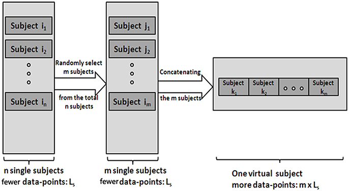
Figure 1. The procedure of generating the V-subjects. Subject i₁ … i_n stands for the total n single subjects, which have few data-points. Subject j₁ … j_m stands for the m subjects selected from the total n subjects. Then the V-subject is the pooling data of the m selected subjects in a random order.

The error of the pLiNGAM algorithm is measured by the false positive ratio (FPR), false negative ratio (FNR), false direction ratio (FDR) and the sum of FPR, FNR, and FDR. FPR stands for the ratio of the number of falsely added edges to the whole possible existing edges, FNR denotes the ratio of the number of falsely missed edges to the whole possible existing edges, and FDR is the ratio of the number of edges that are wrongly identified in the direction to the whole possible existing edges. Furthermore, the sum of FPR, FNR and FDR is calculated to represent the total error of pLiNGAM.

Simulated fMRI Data

The simulated data are from Smith et al. in their 2011 publication (Smith et al., 2011), which have been widely used in fMRI studies (Cole et al., 2010; Smith et al., 2011). The simulations are generated using the Dynamic Causal Modeling fMRI forward model (Friston et al., 2003), in which the Dynamic Causal Modeling uses a nonlinear balloon model (Buxton et al., 1998) for the vascular dynamics. These data can provide 28 simulations, and we select the No. 7 simulation set which has 5000 data points in this paper because it has more than enough data points for the purpose of our study. The No. 7 simulation set contains 5 nodes with 250 min of data at a repetition time of 3 s. The total number of data points is 5000 (scans) for each of the 50 simulated subjects. The coefficients matrix used to generate these 50 subjects data have the same structure with slightly different coefficients.

Real fMRI Data

Participants

12 healthy right-handed young students, including 5 males and 7 females (mean age: 21 years) participate in our study. This study is supported by the Beijing Normal University Imaging Center. All subjects have provided written informed consent.

Data acquisition

Images are acquired using a Siemens Trio 3-Tesla scanner (Siemens, Erlangen, Germany) in the National Key Laboratory for Cognitive Neuroscience and Learning, Beijing Normal University. Participants are instructed to remain motionless, close their eyes but stay awake during the entire scanning procedure which lasts for 8 min. All of the functional data are acquired using an echo-planar imaging sequence with the following parameters: 33 axial slices, TR = 2000 ms, TE = 30 ms, acquisition voxel size, 3.13 × 3.13 × 3.60 mm³, in-plane resolution = 64×64 and matrix = 64 × 64, 240 volumes.

Data analyses

Data preprocessing. The first five volumes of the total 240 volumes in the functional fMRI data are removed to make the signal more stable. Image preprocessing including slice timing, realignment, normalization, and smoothing (FWHM = 8 mm) are conducted using the SPM8 software (http://www.fil.ion.ucl.ac.uk/spm).

Default mode network (DMN) and regions of interest (ROIs). Group ICA is performed to the preprocessed data using the fMRI toolbox (http://mialab.mrn.org/software/#gica) to determine the default mode network (DMN). In recent years, ICA has been widely used to identify the low-frequency neural network during resting-state or cognitively undemanding fMRI scans (Calhoun et al., 2001; Greicius and Menon, 2004; van de Ven et al., 2004). The Group ICA includes two rounds of principal component analysis, ICA separation and back-reconstruction. In ICA separation, the Extended Infomax algorithm is used (Lee et al., 1999). To select the independent component that best matches the DMN, a DMN template is developed based on a dataset of regions reported by Greicius et al. (Greicius and Menon, 2004). Subsequently, the DMN at the single subject level is acquired, and one sample t-test (p < 0.05, false discovery rate corrected) is performed (Figure 2). Figure 2 shows the regions with significant connectivity at the resting state including the medial prefrontal cortex (mPFC), posterior cingulate cortex (PCC), left/right inferior parietal cortex (lIPC/rIPC), left/right lateral and inferior temporal cortex (lITC/rITC), and left/right (para) hippocampus (lHC/rHC). Then, these eight core DMN regions are selected as nodes (ROIs) for the LiNGAM analysis. The coordinates of the eight maximally activated voxels in the core DMN ROIs are given in Table 1, and the ROIs are generated with a sphere with 6 mm-radius centered at the voxel with the maxima local T-value. Then, the data points of each ROI are extracted with the software rest (http://restfmri.net/forum/index.php).

FIGURE 2

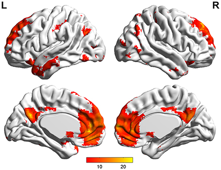
Figure 2. DMN identified by group ICA (p < 0.05, false discovery rate corrected).

TABLE 1

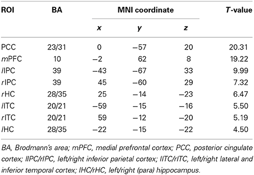
Table 1. The coordinates of all the ROIs for real fMRI data (p < 0.05, false discovery rate corrected).

pLiNGAM on the real fMRI data. Before applying the pLiNGAM on the real fMRI data, the distribution of the V-subject obtained from the real fMRI data is examined by the One-Sample Kolmogorov–Smirnov Test. If the distribution is non-Gaussian, then the LiNGAM will be used on the V-subject to estimate the effective connectivity network among the eight core DMN ROIs.

Results

Simulated Validation

To verify the feasibility of pLiNGAM on the estimation of effective connectivity of fMRI data, some simulation validation are performed, including the desired number of data points that is needed to make the results of LiNGAM stable, the feasibility of the pooling of data points across multiple subjects, the effectiveness of V-subjects in pLiNGAM and the influence of pooling order on pLiNGAM.

Desired number of data points of LiNGAM

The simulated data is used to investigate the desirable number of data points that can make the LiNGAM algorithm stable. Part of the total data points (5000 data points) of each single subject is applied to the LiNGAM. Part of data points in each subject are selected at the beginning of the total data points and the length of the points ranges from 200 to 5000. To avoid the influence of differences between subjects, the LiNGAM algorithm is applied to 50 subjects and the FPR, FNR, and FDR are calculated by averaging the fifty results. The average FPR, FNR, and FDR and the sum of FPR, FNR and FDR are shown in Figure 3 (FDR is 0, so it is not shown in the figure). Three statistical tests: Wald test, chi-square test, and difference chi-square test (p = 0.05) are performed to prune the edges of the estimated network. Figure 3 illustrates that both FPR and FNR are consistently decreasing as the number of data points increases. The sum of FPR and FNR reduces to approximate 7% when the length of data points arrives 5000. Because of the limitation of the number of total data points, this algorithm is not tested with longer data points.

FIGURE 3

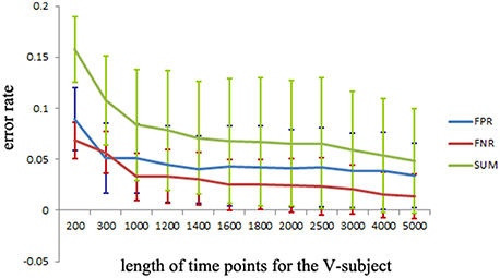
Figure 3. FPR, FNR, FDR and the sum of FPR, FNR, and FDR (SUM) of the simulated subjects with different length of data points for LiNGAM algorithm (FDR is 0, so it is not shown in the figure).

Feasibility of subject pooling

To confirm pooling over subjects' data is a feasible method, the following two validations are performed.

(a) First, test if the pooling step could keep the distribution of the data non-Gaussian. Use the Kolmogorov–Smirnov Test to examine the distribution of the data. For the simulated data, the distribution of each single subject and several V-subjects is tested. The V-subjects were constructed as shown in Figure 1. Each of these V-subjects is pooled with several (range from 1 to 25) single subjects (each with 200 data points), then 25 V-subjects with the length of data points ranging from 200 to 5000 can be constructed. The results of the Kolmogorov–Smirnov Test in Table 2 show that all the single subjects and the V-subjects are significant non-Gaussian distribution. Furthermore, we note that the main difference of the distribution of the single subjects or V-subjects from Gaussian is the “peakedness,” then one classical measurement of the “peakedness” for non-Gaussian distribution named Kurtosis Test is adopted (Hyvärinen and Oja, 2000). The results show that the data has different kurtosis value from 3, e.g., 3.41, 3.98, 4.99 (the kurtosis value of Gaussian distribution is 3), further indicating the deviation of the data from Gaussian distribution. All these results indicate that the V-subjects are feasible to the LiNGAM algorithm.

(b) Second, test if the pooling step could improve the accuracy of the estimated model, in other words, test whether the result of pooling of subjects is better than that of single subject. Three groups of data are modeled: single-subject_2000 (G1), V-subject_2000 (G2), and single-subject_200 (G3). More specifically, the single-subject_2000 group consists of 10 subjects and each single subject has 2000 data points. The V-subject_2000 group is a V-subject with 2000 data points, which are pooled from 10 single subjects with 200 data points each. The single-subject_200 group consists of 10 single subjects and each single subject has 200 data points. The 10 subjects used in this paper are randomly selected from the total 50 subjects and the pooling order is random.

TABLE 2

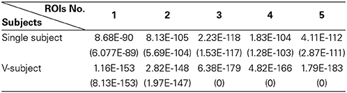
Table 2. The p-value [mean (STD)] of One-Sample Kolmogorov–Smirnov Test of 5 ROIs for the simulated fMRI data.

Then, the FPR, FNR, and FDR of these three groups are calculated, and the sum of FPR, FNR, and FDR for the three groups is shown in Figure 4A. The results clearly show that the G1 group has a smaller sum of FPR, FNR, and FDR compared to the other two groups, and the G2 group has a smaller sum of FPR, FNR, and FDR than the G3 group. Furthermore, one sample t-test is performed on G3 and G1 respectively to verify whether the mean of G3 or G1 is significantly different from G2. The results are encouraging (T = −4.291, p = 0.002 for G1; T = 3.973, p = 0.003 for G3). These statistical results denote that the G1 group shows better results than both the G2 group and G3 group, and G2 group shows better results than G3 group, which indicating that subject pooling is feasible for the LiNGAM algorithm, and pLiNGAM can offer better results when data points were few for the single subjects. Furthermore, to test if the error rate of the G2 group is stable across different subsets of 10 single subjects, 50 V-subject_2000 are constructed by randomly selecting 10 single subjects. The sum of FPR, FNR, and FDR of these V-subject_2000 are then calculated, and the results show that the error rate of the G2 group is stable across different selections of the 10 subjects (Figure 4B).

FIGURE 4

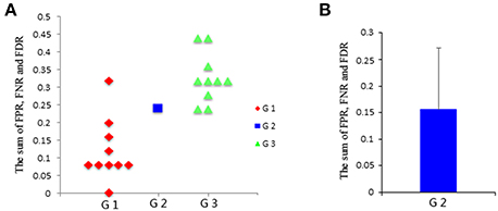
Figure 4. (A) The sum of FPR, FNR, and FDR of three groups: G1: single-subject_2000, G2: V-subject_2000, and G3: single-subject_200; (B) the sum [mean (SD)] of FPR, FNR, and FDR of the G2 group across 50 different V-subject_2000s.

pLiNGAM with V-subjects

To explore the FPR, FNR, and FDR estimated using the pLiNGAM with the V-subjects, the V-subjects are constructed according to the schematic shown in Figure 1. Each of the V-subjects is pooled with several (range from 1 to 25) single subjects (200 data points). For example, in each single subject, 200 data points are selected at the beginning of the total data points, then the 6 single subjects with data points of 200 are combined to form one V-subject with data points of 1200. The length of data points of each V-subject ranges from 200 to 5000. To ensure the reliability of the results, 50 V-subjects are constructed for each length of data points. Figure 5 demonstrates that when data points are more than 2000, the sum of FPR, FNR, and FDR reaches 15%, which is better than most other effective connectivity methods (Cole et al., 2010; Smith et al., 2011).

FIGURE 5

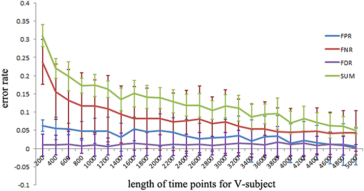
Figure 5. The FPR, FNR, FDR and the sum of FPR, FNR, and FDR (SUM) of the simulated V-subjects for pLiNGAM algorithm. The length of data points of V-subjects ranges from 200 to 5000.

Influence of the pooling order

To determine whether the order of pooling subjects has any effect on the estimated network, the following test is conducted. 10 single subjects are randomly selected from the total 50 subjects. Among 3628800 possible orders, 3000 orders are randomly selected to examine this effect. For each of the 3000 pooling orders, a V-subject is generated. Then, the pLiNGAM algorithm is applied to these V-subjects and the FPR, FNR, and FDR are calculated. Our results show that the estimated network has no relation with the order of pooling, which is consistent with the fact that the major advantage of concatenation of data points across subjects in ICA is ordering the components in different subjects in the same way (Calhoun et al., 2001).

Real fMRI Validation

The distribution of the V-subject from the real fMRI data follows non-Gaussian according to the One-Sample Kolmogorov–Smirnov Test (shown in Table 3). Thus, the pLiNGAM is applicable for the real fMRI data.

TABLE 3

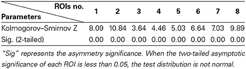
Table 3. The result of One-Sample Kolmogorov–Smirnov Test of 8 ROIs for real fMRI data.

In this section, the stability of causal network is tested on the real fMRI data using pLiNGAM, and the results of effective connectivity for the real fMRI data are also displayed.

The stability of effective connectivity on real fMRI data

pLiNGAM is tested with different subsets of subjects from the real fMRI data to validation the robustness and stability of the result. Several subjects, n = 3 for example, are randomly selected from all the subjects (a total of 12 subjects) to construct the V-subject for 100 times (3, 4, 5, 6, 7, 8, and 9 subjects are tested respectively to ensure the procedure of random selection be repeated for 100 times, while 1, 2, 10, 11, 12 subjects can't be randomly selected for 100 times and are not used for testing). For each number of subjects, the causal network is analyzed for 100 times, and the common structure of the 100 causal networks is then considered as a baseline to calculate the FPR, FNR, and FDR of each causal network. Then the average of the sum of the FPR, FNR, and FDR is taken as the variability of the results. As it is shown in Figure 7, the variability of different subsets of the subjects is not high (about 0.26 for different number of subjects). This variability is comparable with the results of many algorithms that are mentioned in Smith et al., such as Granger, Bayes net and so on (Smith et al., 2011). Furthermore, the variability of different subsets of the subjects is stable along with the increased number of subjects (slightly decrease). These results indicate the stability and robustness of the causal networks that obtained by pLiNGAM.

The results of effective connectivity for real fMRI data

Figure 6 shows the effective connectivity model of DMN during the resting state investigated by the pLiNGAM algorithm (using all the 12 subjects). From Figure 6, we can conclude the following connections: mPFC→rHC/rIPC/lITC/PCC/rITC/lIPC/lHC, rIPC→PCC/rHC/lHC/lITC, rITC→rIPC/lIPC/PCC/lITC/lHC/rHC, lITC→PCC/lHC/rHC, lIPC→PCC/rIPC/rHC/lHC/lITC (p < 0.05, Wald statistics). Seven direct connections are detected between mPFC, rHC, rITC, lHC, lIPC, PCC, and the other ROIs. Interestingly, all links associated with mPFC are out-going connections, and all links associated with rHC are in-going connections. Furthermore, six of the total seven links associated with rITC are out-going connections, and six of the total seven links associated with lHC are in-going connections. In addition, five of the total seven links associated with lIPC are out-going connections, and five of the total seven links associated with PCC are in-going connections.

FIGURE 6

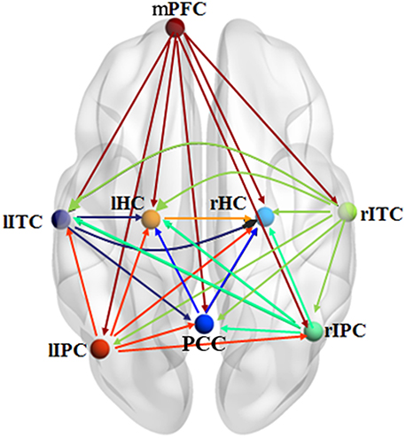
Figure 6. Effective connectivity model of DMN during the resting state explored by pLiNGAM. The different line colors indicate connections originating from different nodes. The effective connectivity has been corrected using Wald statistics, chi-square test and difference chi-square test with p < 0.05 as the significant level.

Discussion

This study employs the pLiNGAM algorithm to explore the effective connectivity of fMRI data with the V-subject. The results demonstrate that the pLiNGAM is feasible for both simulated and real fMRI data.

The pLiNGAM algorithm has several advantages in estimating the effective connectivity of brain areas. First, the simulated fMRI data demonstrate that pLiNGAM produces a more robust effective connectivity model with the V-subject than the original single subject. With a small number of data points, however, the computational stability of pLiNGAM cannot be guaranteed because in ICA estimation, the weight matrix B often converges on different values when there are not enough data points (Goebel et al., 2003). Second, this algorithm is based on the assumptions of non-Gaussianity of disturbance variables, linearity and an acyclic model, which allow the identification of the full causal model. Previous methods (Pearl, 2000; Shimizu and Kano, 2008) based on the assumption of Gaussianity require additional information (such as the causal order of variables) to obtain a full causal model (Shimizu et al., 2006). Third, a V-subject composed of more than one subject can provide more valuable information compared to a single subject. Fourth, the sum of FPR, FNR and FDR for the V-subjects can fall to 15% (Figure 5), which is smaller than most of other approaches (45%) (Cole et al., 2010; Smith et al., 2011).

Our results of the simulated data show that the sum of FPR, FNR, and FDR can just reduce to approximate 7% but not 0% when there are sufficient number of data points (shown in Figure 5), indicating that we can't obtain a perfect network of the simulated data even if the data points are long enough. This situation is explainable. A sampling step was done in the procedure of generating the simulated data (Smith et al., 2011), thus may result in the loss of information about the data. Furthermore, some noises are also added into the simulated data (Smith et al., 2011). All these process may cause the imperfect performance of pLiNGAM even when the data points are long enough.

The subject pooling has been verified to be a reasonable method through the simulated fMRI data. Then this method is applied to the real fMRI data, and the results show that the causal network is reliable and stable across different subsets of subjects, which further indicated the feasible application of pLiNGAM in the situation with low inter-subject variability. Furthermore, most of the links associated with the PCC are in-going connections, demonstrating that the PCC acts as a confluent node. Similar conclusions have been acquired in the previous studies (Li et al., 2012; Yan et al., 2013). In addition, the links associated with mPFC show good consistency because all links are out-going connections. Li et al.'s (2012) study also supports this result.

The variability in Figure 7 for the real fMRI data is not significantly decreasing (slightly decreasing) as the number of subjects increases, which is different from the results of the V-subject in Figure 5. This may because that the variability in the real fMRI data is more stable than that of the simulated data, thus having reached the flat part toward the tail like that in Figure 5. To a certain extent, the variability is stable (slightly decrease) along with the increased number of subjects for the real fMRI data, which indicates the stability and robustness of the causal networks that obtained by pLiNGAM. In any way, further detailed explorations are needed to delve into this problem in our future study.

FIGURE 7

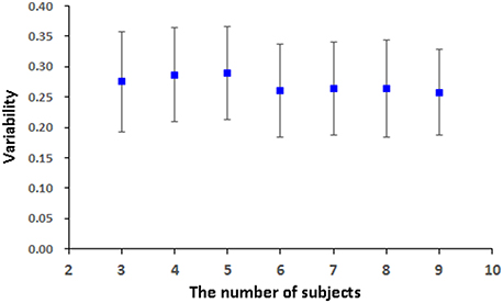
Figure 7. The variability [mean (STD)] of the 100 V-subjects constructed from different number of subjects (3, 4, 5, 6, 7, 8, and 9 respectively) for the real fMRI data with pLiNGAM algorithm.

While having many merits, the pLiNGAM method still has several limitations. First, it only performs well when the inter-subject variability is low. pLiNGAM is one form of the “VTS” technique (Li et al., 2008), which assumes that every subject within a group performs the same function and has the same connectivity network. Other group analysis method based on LiNGAM, such as the algorithm proposed in Shimizu (2012), assumes that each subject shares a causal ordering but different connection strengths, which is similar with the “CS” approach (Li et al., 2008). So this algorithm in Shimizu (2012) may perform worse than pLiNGAM when the inter-subject variability is low (e.g., the healthy subject group), while better than pLiNGAM when inter-subject variability is a little larger (e.g., patient group). Therefore, more efforts are needed to improve pLiNGAM in order to be applicable for more general situations. Second, the V-subjects have more data points, thus may result in longer calculation time. In addition, the calculation time also depends on group sizes and the number of ROIs (Hyvärinen and Oja, 1997). Third, the assumption of an acyclic model may be a limitation to the fMRI data. This assumption implies that information can only be transmitted from one ROI to another, but not transmitted back. However, feedback is an important feature for biological systems, such as cortico-subcortical loops (Lynch and Tian, 2006). In any way, further exploration is needed to improve the pLiNGAM algorithm.

Conflict of Interest Statement

The authors declare that the research was conducted in the absence of any commercial or financial relationships that could be construed as a potential conflict of interest.

Acknowledgments

This work was supported by the Key Program of National Natural Science Foundation of China (91320201), the Funds for International Cooperation and Exchange of the National Natural Science Foundation of China (61210001), the Excellent Young Scientist Program of China (61222113), and Program for New Century Excellent Talents in University (NCET-12-0056).

References

Baker, J. R., Weisskoff, R. M., Stern, C. E., Kennedy, D. N., Jiang, A., Kwong, K. K., et al. (1994). “Statistical assessment of functional MRI signal change,” in Proceedings of the 2nd Annual Meeting of the Society of Magnetic Resonance, 626.

Biswal, B., Zerrin Yetkin, F., Haughton, V. M., and Hyde, J. S. (1995). Functional connectivity in the motor cortex of resting human brain using echo-planar mri. Magn. Reson. Med. 34, 537–541. doi: 10.1002/mrm.1910340409

Pubmed Abstract | Pubmed Full Text | CrossRef Full Text | Google Scholar

Bollen, K. A. (1998). Structural Equation Models. John Wiley & Sons, Ltd.

Google Scholar

Buxton, R. B., Wong, E. C., and Frank, L. R. (1998). Dynamics of blood flow and oxygenation changes during brain activation: the balloon model. Magn. Reson. Med. 39, 855–864. doi: 10.1002/mrm.1910390602

Pubmed Abstract | Pubmed Full Text | CrossRef Full Text | Google Scholar

Calhoun, V. D., Adali, T., Pearlson, G. D., and Pekar, J. J. (2001). A method for making group inferences from functional MRI data using independent component analysis. Hum. Brain Mapp. 14, 140–151. doi: 10.1002/hbm.1048

Pubmed Abstract | Pubmed Full Text | CrossRef Full Text | Google Scholar

Chen, Y., Bressler, S. L., Knuth, K. H., Truccolo, W. A., and Ding, M. (2006). Stochastic modeling of neurobiological time series: power, coherence, Granger causality, and separation of evoked responses from ongoing activity. Chaos 16, 26113. doi: 10.1063/1.2208455

Pubmed Abstract | Pubmed Full Text | CrossRef Full Text | Google Scholar

Cole, D. M., Smith, S. M., and Beckmann, C. F. (2010). Advances and pitfalls in the analysis and interpretation of resting-state FMRI data. Front. Syst. Neurosci. 4:8. doi: 10.3389/fnsys.2010.00008

Pubmed Abstract | Pubmed Full Text | CrossRef Full Text | Google Scholar

Comon, P. (1994). Independent component analysis, a new concept? Signal Process 36, 287–314. doi: 10.1016/0165-1684(94)90029-9

CrossRef Full Text | Google Scholar

Friston, K. J. (1994). Functional and effective connectivity in neuroimaging: a synthesis. Hum. Brain Mapp. 2, 56–78. doi: 10.1002/hbm.460020107

CrossRef Full Text | Google Scholar

Friston, K. J., Frith, C. D., Liddle, P. F., and Frackowiak, R. (1993). Functional connectivity: the principal-component analysis of large (PET) data sets. J Cerebr Blood F Met 13, 5. doi: 10.1038/jcbfm.1993.4

Pubmed Abstract | Pubmed Full Text | CrossRef Full Text | Google Scholar

Friston, K. J., Harrison, L., and Penny, W. (2003). Dynamic causal modelling. Neuroimage 19, 1273–1302. doi: 10.1016/S1053-8119(03)00202-7

Pubmed Abstract | Pubmed Full Text | CrossRef Full Text | Google Scholar

Geiger, D., and Heckerman, D. (1994). “Learning gaussian networks,” in Proceedings of the 10th International Conference on Uncertainty in Artificial Intelligence (Morgan Kaufmann Publishers Inc.), 235–243.

Goebel, R., Roebroeck, A., Kim, D., and Formisano, E. (2003). Investigating directed cortical interactions in time-resolved fMRI data using vector autoregressive modeling and Granger causality mapping. Magn. Reson. Imaging 21, 1251–1261. doi: 10.1016/j.mri.2003.08.026

Pubmed Abstract | Pubmed Full Text | CrossRef Full Text | Google Scholar

Goncalves, M. S., Hall, D. A., Johnsrude, I. S., and Haggard, M. P. (2001). Can meaningful effective connectivities be obtained between auditory cortical regions? Neuroimage 14, 1353–1360. doi: 10.1006/nimg.2001.0954

Pubmed Abstract | Pubmed Full Text | CrossRef Full Text | Google Scholar

Greicius, M. D., Krasnow, B., Reiss, A. L., and Menon, V. (2003). Functional connectivity in the resting brain: a network analysis of the default mode hypothesis. Proc. Natl. Acad. Sci. U.S.A. 100, 253–258. doi: 10.1073/pnas.0135058100

Pubmed Abstract | Pubmed Full Text | CrossRef Full Text | Google Scholar

Greicius, M. D., and Menon, V. (2004). Default-mode activity during a passive sensory task: uncoupled from deactivation but impacting activation. J. Cogn. Neurosci. 16, 1484–1492. doi: 10.1162/0898929042568532

Pubmed Abstract | Pubmed Full Text | CrossRef Full Text | Google Scholar

Heckerman, D. (2008). “A tutorial on learning with Bayesian networks,” in Innovations in Bayesian Networks (Berlin; Heidelberg: Springer), 33–82.

Google Scholar

Hyvärinen, A., and Oja, E. (1997). A fast fixed-point algorithm for independent component analysis. Neural Comput. 9, 1483–1492. doi: 10.1162/neco.1997.9.7.1483

CrossRef Full Text | Google Scholar

Hyvärinen, A., and Oja, E. (2000). Independent component analysis: algorithms and applications. Neural Netw. 13, 411–430. doi: 10.1016/S0893-6080(00)00026-5

Pubmed Abstract | Pubmed Full Text | CrossRef Full Text | Google Scholar

Kim, J., Zhu, W., Chang, L., Bentler, P. M., and Ernst, T. (2007). Unified structural equation modeling approach for the analysis of multisubject, multivariate functional MRI data. Hum. Brain Mapp. 28, 85–93. doi: 10.1002/hbm.20259

Pubmed Abstract | Pubmed Full Text | CrossRef Full Text | Google Scholar

Lee, T., Girolami, M., and Sejnowski, T. J. (1999). Independent component analysis using an extended infomax algorithm for mixed subgaussian and supergaussian sources. Neural Comput. 11, 417–441. doi: 10.1162/089976699300016719

Pubmed Abstract | Pubmed Full Text | CrossRef Full Text | Google Scholar

Li, J., Li, R., Chen, K., Yao, L., and Wu, X. (2012). Temporal and instantaneous connectivity of default mode network estimated using Gaussian Bayesian network frameworks. Neurosci. Lett. 513, 62–66. doi: 10.1016/j.neulet.2012.02.008

Pubmed Abstract | Pubmed Full Text | CrossRef Full Text | Google Scholar

Li, J., Wang, Z. J., and McKeown, M. J. (2007). “A multi-subject, dynamic Bayesian networks (dbns) framework for brain effective connectivity,” in Acoustics, Speech and Signal Processing, IEEE International Conference, 429–432.

Google Scholar

Li, J., Wang, Z. J., Palmer, S. J., and McKeown, M. J. (2008). Dynamic Bayesian network modeling of fMRI: a comparison of group-analysis methods. Neuroimage 41, 398–407. doi: 10.1016/j.neuroimage.2008.01.068

Pubmed Abstract | Pubmed Full Text | CrossRef Full Text | Google Scholar

Lynch, J. C., and Tian, J. (2006). Cortico-cortical networks and cortico-subcortical loops for the higher control of eye movements. Prog. Brain Res. 151, 461–501. doi: 10.1016/S0079-6123(05)51015-X

Pubmed Abstract | Pubmed Full Text | CrossRef Full Text | Google Scholar

McLntosh, A. R., and Gonzalez Lima, F. (1994). Structural equation modeling and its application to network analysis in functional brain imaging. Hum. Brain Mapp. 2, 2–22. doi: 10.1002/hbm.460020104

Pubmed Abstract | Pubmed Full Text | CrossRef Full Text | Google Scholar

Mechelli, A., Penny, W. D., Price, C. J., Gitelman, D. R., and Friston, K. J. (2002). Effective connectivity and intersubject variability: using a multisubject network to test differences and commonalities. Neuroimage 17, 1459–1469. doi: 10.1006/nimg.2002.1231

Pubmed Abstract | Pubmed Full Text | CrossRef Full Text | Google Scholar

Pearl, J. (2000). Causality: Models, Reasoning and Inference. Cambridge: MIT press.

Google Scholar

Shachter, R. D., and Kenley, C. R. (1989). Gaussian influence diagrams. Manage. Sci. 35, 527–550. doi: 10.1287/mnsc.35.5.527

CrossRef Full Text | Google Scholar

Shimizu, S. (2012). Joint estimation of linear non-Gaussian acyclic models. Neurocomputing 81, 104–107. doi: 10.1016/j.neucom.2011.11.005

CrossRef Full Text | Google Scholar

Shimizu, S., Hoyer, P. O., Hyvärinen, A., and Kerminen, A. (2006). A linear non-Gaussian acyclic model for causal discovery. J. Mach. Learn. Res. 7, 2003–2030.

Pubmed Abstract | Pubmed Full Text | Google Scholar

Shimizu, S., and Kano, Y. (2008). Use of non-normality in structural equation modeling: application to direction of causation. J. Stat. Plan. Infer. 138, 3483–3491. doi: 10.1016/j.jspi.2006.01.017

CrossRef Full Text | Google Scholar

Smith, S. M., Miller, K. L., Salimi-Khorshidi, G., Webster, M., Beckmann, C. F., Nichols, T. E., et al. (2011). Network modelling methods for FMRI. Neuroimage 54, 875–891. doi: 10.1016/j.neuroimage.2010.08.063

Pubmed Abstract | Pubmed Full Text | CrossRef Full Text | Google Scholar

Spirtes, P., Glymour, C. N., and Scheines, R. (2000). Causation, Prediction, and Search. MIT press.

Google Scholar

van de Ven, V. G., Formisano, E., Prvulovic, D., Roeder, C. H., and Linden, D. E. (2004). Functional connectivity as revealed by spatial independent component analysis of fMRI measurements during rest. Hum. Brain Mapp. 22, 165–178. doi: 10.1002/hbm.20022

Pubmed Abstract | Pubmed Full Text | CrossRef Full Text | Google Scholar

Wu, D., and Lewin, J. S. (1994). “Evaluation of non-parametric statistical measures and data clustering for functional MR data analysis,” in Proceedings of the SMR 2nd Annual Meeting (San Francisco, CA), 629.

Yan, H., Zhang, Y., Chen, H., Wang, Y., and Liu, Y. (2013). Altered effective connectivity of the default mode network in resting-state amnestic type mild cognitive impairment. J. Int. Neuropsychol. Soc. 19, 400–409. doi: 10.1017/S1355617712001580

Pubmed Abstract | Pubmed Full Text | CrossRef Full Text | Google Scholar

Zheng, X., and Rajapakse, J. C. (2006). Learning functional structure from fMR images. Neuroimage 31, 1601–1613. doi: 10.1016/j.neuroimage.2006.01.031

Pubmed Abstract | Pubmed Full Text | CrossRef Full Text | Google Scholar