Sensor selection and chemo-sensory optimization: toward an adaptable chemo-sensory system

Introduction

The idea to mirror the biological senses, particularly the biological sense of olfaction, with artificial electronic systems has been a human dream for many years (Persaud and Dodd, 1982; Gardner and Bartlett, 1999). The choice of olfaction is not coincidental. While for humans, whose vision and hearing senses are their primary mode of communication with the outside world, olfaction is a rather little used sense, as demonstrated by the relatively normal lives led by people with anosmia – people who cannot smell – for most of the animals, olfaction is the primary means of exploration and communication (Bhandawat et al., 2007). The biggest challenge in performing such an imitation, though, is how to reliably emulate this system by understandable artificial mechanisms, commonly referred to as electronic noses (e-nose). e-Nose, or their odorant chemo-receptors to be more precise, play an important role in this challenge not only because they serve as oversimplified, yet accurate, reproductions, and simulations of the biological sense of olfaction, but also because these artifacts are able to non-invasively detect, acquire, interpret, select, and organize the sensory information of certain situations that humans can not perceive or understand (Persaud and Dodd, 1982; Freund and Lewis, 1995; Dickinson et al., 1996; Gardner and Bartlett, 1999). The capabilities of odor chemo-sensors are broad and include many challenging tasks such as discriminating organic compounds with chain lengths that differ by a single carbon atom (White et al., 1996; Persaud and Travers, 1997). However, their limitations in characterizing odor-stimuli, including the poor sensitivity to analytes and the lack of reproducibility in their responses in repeated trials, are still very serious (Moseley and Tofield, 1987). With the advent of the latest technological breakthroughs, recent progress in chemical micro-sensory systems has been stimulated by inter-disciplinary perspectives at the intersection of materials science, micro- and nano-technology, microelectronics, and signal processing/pattern recognition in an attempt to ameliorate these apparent limitations. For example, the effect of microstructure, size feature of the material, the advantages of nano-structured materials (e.g., nanowires, nanorods, nanoribbons), and the efforts to functionalize sensing materials by adding catalysts have been widely studied from the material perspective to improve the sensors’ sensitivity and selectivity as well as to reduce their power consumption and time of response (Yamazoe, 2005; Franke et al., 2006; Comini et al., 2009; Gurlo, 2010; Stoycheva et al., 2011). On the other hand, different feature selection, feature extraction, and pattern-recognition techniques, from the signal processing and machine learning viewpoint, have also been implemented with remarkable results in many critical applications (Di Natale et al., 1995; Eklöv et al., 1997; Nakamoto et al., 1997; Gutierrez-Osuna et al., 1999; Muezzinoglu et al., 2009; Vergara et al., 2011). However, while maintaining and expanding this fruitful interaction is essential for solving these problems ahead, this collaborative platform will be lacking a key player until the material and hardware development component improves, since the current sensory modalities available do not meet the power consumption and dimension restrictions required for particular real-time applications. Therefore, among the many different strategies implemented in the literature, interacting with the conditioning parameters at the sensor level (e.g., working temperature for metal-oxide gas sensors) is the only viable solution to overcome these annotated problems (Moseley and Tofield, 1987).

In principle, almost every odorant-sensing technology offers the advantage of being tunable through the selection of parameter values. Interacting with such parameters influences many critical qualities of the measurement, including sensitivity to analytes and reproducibility. For example, the temperature-modulation technique for metal-oxide gas sensors, takes advantage of such a relationship to enrich the information content of the sensor, since it directly alters the reaction kinetics at the sensor surface in the presence of an odorant (Sears et al., 1989a,b, 1990; Nakata et al., 1992, 1996, 1998; Semancik and Cavicchi, 1999). A thorough understanding of how such interactions take place in the chemo-sensory system requires quantitative characterizations of the response of individual sensors, both within and among chemical stimuli. This approach will enable us to generalize the relationship between the control variable and the target quality.

Once the odorant-sensing/parameter interaction is known (or can be inferred from previous observations), a natural venue to follow is the optimization of the chemo-sensory system with respect to a solid criterion that properly expresses the observed goal. A number of approaches under the notion of optimization have been implemented in the literature, but only a handful of authors have approached the problem in a systematic fashion. In this context, the purpose of this paper is to provide the reader with a critical review of the different efforts that have been made in the context of sensor selection and sensor optimization in the chemo-sensing community for the last years. We will be visiting these criteria individually as we proceed further in this review.

Before embarking upon the subject of optimization, we would like to make a final point in the context of terminology. The label “optimization” has been very popular for many years to describe the terms of “sensor optimization” and “sensor-array optimization” interchangeably. We believe, however, that this terminology can be very misleading, since the former mostly refers to finding the “optimal operational condition” of the sensor device, whereas the latter usually means selecting an “optimal” combination of sensors between a potentially large pool of different sensors that are best suited to the identification task – pretty much as feature selection. Therefore, although these two groups of procedures are fully complementary and valuable tools to analyze our chemical sensors, they deserve to be treated as separate topics. For this reason, we organize the structure of this review according to which of these two aspects of “adaptation” (or sensor optimization among many other names considered) is taking place at the sensor level. It is not say that this adaptation can occur only at one or another side of the coin; sensor optimization may also involve coordination of other aspects, such as the adaptability of the chemical sensors at multiple levels and time scales through their operating parameters targeted when the environmental conditions change. Accordingly, we have decided to give three more specific threads to run this review. The first is gain control in those methods that have been implemented to optimize the chemical sensors when used as a sensor array. The second, which is the other side of the same coin, is a functional analysis of the coding schemes used in the optimization of each chemical sensor individually. And the third is a systematic analysis of the advantages derived from the coding scheme used by the early optimization stages implemented on chemical sensors in an active fashion, or the so-called adaptive sensing optimization. Finally, in order to gain a better understanding of how the optimization processes are occurring at the sensor level, or even to discuss whether the processes are or are not working, we have included an overview of the operating temperature dependence for the response of semiconductor gas sensors at the beginning of the Section “Metal-oxide Gas Sensors and Their Operation: Initial Optimization Methods.” We strongly recommend people who may not be familiarized with the functioning process of chemical sensors, specifically metal-oxide gas sensors, to review this section.

Metal-Oxide Gas Sensors and Their Operation: Initial Optimization Methods

Metal-Oxide Gas Sensors and Temperature Dependence

Undoubtedly, metal-oxide gas sensors have become one of the most widely used sensing technologies in machine olfaction for a diversity of applications. Because of the strict and highly deterministic dependence of the sensor response on its operating temperature, governing the basic operating principle of this sensing technology, we believe that it is worthwhile to provide a good insight into the dynamic behavior and operating principle of metal oxide sensors so we can get a better understanding of how the optimization processes described here take place at the sensor level. Accordingly, the followings lines of this section feature the basic operating principle of the said chemo-sensing technology. The sensitive layer, in this case the metal-oxide film that is made of particles that range from nanometers up to microns, possesses two operating mechanisms. The former is associated with an ideally specific interaction of the surface with the target analyte, whilst the latter refers to an effective transduction of the bulk conductance. If the interaction takes place exclusively at the surface of the sensitive layer, then the bulk conductivity does not contribute and represents only a shunt which decreases the signal-to-noise ratio. On the other hand, for materials in which interaction originates in the bulk of the sensitive layer, the response of the sensor, and in particular its time of response, is affected by the thickness and porosity of the material, giving faster response times for thin films than for thick films (Yamazoe, 2005; Franke et al., 2006; Stoycheva et al., 2011). Accordingly, for a given type of base material, the sensor property sensitively depends on the structural features, the presence and state of catalytically active surface dopants, and the working temperature.

The central reaction mechanism responsible for most of the chemical compound responses/interactions involves changes in the concentration of surface oxygen species, such as O²⁻ (Göpel, 1985, 1988; Göpel et al., 1991). The formation of such ions means that the oxygen adsorbed at the gas/solid interface abstracts electrons from the conduction band of the sensing material, which results in the development of Schottky potential barriers at the grain boundaries. In the case of an n-type semiconductor such as SnO₂, on the one hand, the electrons come from ionized donors via the conduction band, the charge-carrier density at the interface is reduced, and a potential barrier to charge transport, ΔΦ, develops. At the junctions between the grains of the solid (see Figure 1), the depletion layer and the associated potential barrier are responsible for high resistance contacts which dominate the resistance of the sensor. Thus, depending on the temperature, oxygen is ionosorbed on the surface predominantly as O₂₋ ions below 150°C, or as O⁻ ions between 150 and 400°C, which is the general operating temperature range. Above 400°C, the parallel formation of O²⁻ occurs, which is then directly incorporated into the lattice above 600°C (Barsan et al., 1999). In the case of a p-type oxide, on the other hand, adsorbed oxygen acts as a surface acceptor state, abstracting electrons from the valence band, and hence giving rise to an increase in the charge-carrier (holes) concentration.

FIGURE 1

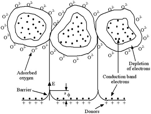
Figure 1. Structural and band model showing the role of intergranular contact regions in determining the conductance over a polycrystalline metal-oxide semiconductor. Three grains with adsorbed oxygen providing surface depletion layers. The depleted layers are responsible for a high contact resistance. For conduction, electrons must cross over the surface barriers.

In response to an analyte and under stationary conditions (i.e., without humidity, constant flow, and fixed operating temperature), the sensor involves an exponential change in the conductance/resistance across its sensing layer. This resulting change can be interpreted as a shift of the state of equilibrium of the surface oxygen reaction due to the presence of the target analyte, which can be either a reducing or oxidizing specie. The response of semiconductor gas sensors to reducing species implies a change in the concentration of adsorbed oxygen species. On the other hand, oxidizing species can interact with the sensor surface in a variety of ways; for example, interacting directly with the surface and forming negatively charged ionosorbed species or in competition with ionosorbed oxygen or oxygen ions for the adsorption sites available (Ruhland et al., 1998). These changes modulate the height of the potential barriers and thus the conductance of the sensing layer. The reason these characteristic conductance–temperature profiles arise is summarized as follows:

• There are different adsorbed oxygen species such as O⁻, O²⁻, and O₂₋ over the temperature range (Sears et al., 1989a; Barsan et al., 1999).

• Different gases have different optimum oxidation temperatures (Moseley and Tofield, 1987).

• Adsorption, desorption, and diffusion rates (of oxygen species, reducing and oxidizing gases, and oxidation by-products) are temperature-dependent (Clifford and Tuma, 1983; Nakata et al., 1991; Wlodek et al., 1991).

Accordingly, when the operating temperature of the sensor varies, the kinetics of adsorption, desorption, and reaction occurring at the sensor surface in the presence of atmospheric oxygen and other reducing or oxidizing species is altered. This approach leads to sensor responses (e.g., transient conductance patterns) that are characteristic of the species present in the gas mixture. Having such an easy way of interacting with the sensor and its characteristics justifies the use of temperature as a control variable in a deterministic setting and, thus, the optimization of the sensor device with respect to this parameter (i.e., the sensor’s operating temperature).

Initial Methods

More than two decades have passed since Parsaud’s pioneering publication on machine olfaction and e-nose appeared in literature (1982). Researchers have since devoted their work to developing signal processing procedures and optimization strategies to ameliorate the performance of metal-oxide gas sensors. This section presents an introduction to such first deployed optimization methods. One of the pioneering works was presented by Corcoran et al. (1998), who applied a triangular waveform (4.16 mHz) to modulate the operating temperature of eight commercially available gas sensors (from Figaro Engineering Inc., Japan, http://www.figaro.co.jp) between 250 and 500°C. They extracted features from the sensor transients using two different approaches. The first approach consisted of sub-sampling the response transients obtaining a 26-point vector (equivalent to 10°C steps) per transient. The second one, on the other hand, consisted of calculating eight secondary features from each response transient, such as the time to maximum value, time to minimum value, maximum positive slope, etc. They implemented then an optimization procedure to determine which sensors and features should be used to better classify the aromas from three loose leaf teas using a neural network classifier. The optimization process consisted of applying genetic algorithms (GAs) for variable selection (Davis, 1991). By applying this technique, the authors showed that it was possible to reach a high success rate in tea classification (93%) using only 21 dynamic features out of the 208 available features. However, the optimization of the temperature-modulating signal (frequency, temperature range, and waveform type) was not considered at the time by the authors. Had this optimization been envisaged, further improvements in classification performance would have been obtained.

More recently, Fort et al. (2002) and Fort et al. (2003) used temperature-modulated metal-oxide gas sensors (sensors modulated with a pure sinusoidal signal) to show that the selection of the signal frequency was of paramount importance for gas identification. The authors demonstrated that if the temperature of the sensors is varied relatively quickly in comparison with the chemical response time, the sensor resistance varies as a function of the temperature with an exponential law characteristic to metal oxides. AS a result, the response shape would have only a slight dependence on the chemical environment. On the other hand, when the operating temperature varies slowly enough in comparison to the chemical response time, the response profile gives a series of quasi-stationary chemical responses. The best discrimination among the species studied (vapors from water solutions containing ethanol and other volatile organic compounds) can be obtained then by selecting a temperature profile with a period close to that for the chemical response time of the sensor. Accordingly, these results suggested that the effectiveness of the temperature-modulation analysis depends on the period of the sine wave, which must be chosen in agreement to the chemical reaction rate of each sensor. Around the same time, Choi et al. (2002) and Huang et al. (2003) got similar results that the ones presented above. The authors evaluated the effect of utilizing different kind of temperature modulation signals, such as pulse, trapezoid, triangular, and saw-tooth, as well as modulating frequency values in the sensor response performance. In particular, utilizing different modulating frequencies values (50, 30, 40, and 20 mHz), Huang et al. (2003) experimentally demonstrated that different and more odor specific response patterns were developing in the sensor response as the modulating frequency was taken nearer to low values (e.g., 20 mHz), suggesting that low-frequency temperature modulation signals are more relevant to alter the kinetics of adsorption, diffusion, and reaction phenomena (i.e., the interaction of odorous compounds and the gas-sensitive surface) occurring at the sensor surface.

Sensor-Array Optimization

A wide variety of sensors, feature extraction, and feature selection methods that are available to the experimenter when considering a new sensing problem have been described elsewhere in the literature (Guyon and Elisseeff, 2003; Rodriguez-Lujan et al., 2010; Vergara and Llobet, 2011). However, when one is working with an array of non-specific sensors, the biggest concern to the experimenter is the number of sensors needed to form a chemo-sensory array. One manner to approach this dilemma might be to augment an existing array by adding sensors appropriate to the new task. However, this is actually a computationally expensive and potentially wasteful solution because using more sensors does not necessarily guarantee improvement in the overall performance. As a consequence, the most conceivable way to address this issue is to design an optimal array of sensors (even comprising completely different sensing technologies) that would promote the maximum accuracy with which the sensory system can estimate the stimulus or optimally discriminate between neighboring stimuli. A number of theoretical studies have been performed with the notion of “array optimization” and are now available in the literature, where can be explored when the experimenter is approaching to a new odor identification scenario. One of the pioneering investigations in this context is the one presented by Zaromb and Stetter (1984), who proposed, over 20 years ago, a theoretical model to estimate the minimum number of parameter P = (S sensors × M operating modes) that would be required to discriminate a mixture of up to A analytes from a pool of n different odorants. By assuming that the response of each sensor is noiseless and binary related to each odor stimulus (i.e., response/no response), they argued for a combinatorial measure of the number of sensors required to detect a given number of chemical species as

The authors, whose work was subsequently corroborated by Alkasab et al. (2002), proposed a “rule of thumb” in their work according to which sensors and operating modes should be selected so that each of the P parameters does not respond to more than P/A individual compounds. Later, in a seminal paper presented by Niebling and Müller (1995), the authors proposed the use of an inverse feature space to design sensor arrays. In this inverse feature space, each of the n analytes was represented as a separate dimension, and each of the s sensors was then represented as a point in this n-dimensional space. They showed that this visual representation should enable the experimenter to detect potential discrimination problems and to design new sensors to adequately address these problems. Gardner and Bartlett (1996) proposed a computational model for cross-selective sensors that also considers the effects of noise and errors. By using the ratio between the total volume of the sensor space and the volume made up by the sensor errors, the authors estimated an upper limit of the number of analytes that can be discriminated by the given array. As a final result, they proposed a measure of performance, which was essentially equivalent to the classical Fisher’s linear discriminant analysis (LDA) ratio (i.e., the ratio of between-class distance to within-class variance).

It was not until the early 2000s when Pearce and Sanchez-Montañes (2003) implemented for the first time an information-theoretic approach for the optimization of chemo-sensory array systems. In particular, they demonstrated how the “tunings” of individual sensors may affect the overall performance of the array. In order to demonstrate the effects of noise and tuning on array performance, they incorporated the concept of “hyper-volume of accessible sensor space” (V_S), a volume in the sensor space that contains the sensor-array response to a specific set of analytes. As Figure 2A suggests, for a three-odor by two-sensor problem, the collinearity limits the number of possible sensor responses. Therefore, the maximum number of analyte mixtures that can be discriminated by the array is limited by the ratio between V_S and V_N (the hyper-volume defined by the accuracy of the sensor array; see Figure 2B).

FIGURE 2

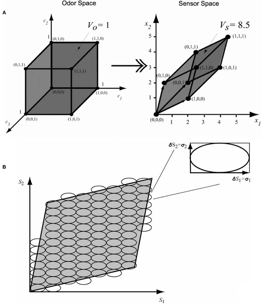
Figure 2. (A) Visualization of a three-odor-to-two-sensor transformation. (B) The maximum number of feature vectors that can be discriminated is the ratio between the hyper-volume of the accessible sensor space (V_S) and the accuracy of the sensor-array response. Figure reproduced with permission from Pearce and Sanchez-Montañes (2003) Copyright 2003 Wiley-VCH, Weinheim.

Assuming that the errors/noise ratio does not exhibit any correlation with the analyte stimulus, the authors showed then that the geometric interpretation in Figure 2 can be expressed by means of the Fisher information (FI) matrix defined as

where c is a vector containing the concentration of the analytes, x is the response of the sensor array to the stimulus c, and p(x|c) is the conditional probability of observing the sensor response x upon a given stimulus c. FI is important in this context because it provides a lower bound (i.e., best-case case) on the accuracy with which the stimulus, c, can be predicted from the sensor response x. This lower limit is determined as

where “var” means the variance, and ĉ is the estimation/prediction of the component i of c, i = 1, …, N. This result was called the “Cramér–Rao Bound” and limits the performance of the best unbiased estimator that can be built.

In order to use these theoretical constructs in practice, the first stage one should perform is the formal description of the sensory context C and a clear specification of the task. The context C, on one hand, quantitatively describes the likelihood of occurrence of each odor stimulus, whereas the chemo-sensory task, on the other hand, is an interpretation of the sensory response (i.e., a quantification or identification task). Once the sensory context and task are properly defined, one then would assume a parametric density p(x|c) for each individual sensor, estimate the parameters from experimental data (i.e., by measuring the sensor-array responses to a number of analyte mixtures), compute the FI using Eq. 2, and finally compute the expected accuracy of the array using Eq. 3. This resulted accuracy estimate would then be used as a “figure of merit” to select an optimal array configuration from a pool of cross-selective sensors. Once the “optimal” array condition is found, a catalog of parameters for each sensor used within practical systems today may then be envisaged, which would make the optimization of sensory array systems to particular detection tasks a simple routine operation.

More recently, in the same domain of information theory, Muezzinoglu et al. (2010) introduced a sensor-array optimization scheme for odor identification. The authors demonstrated the effects of tuning the sensor’s operating parameter in a chemo-sensory array by incorporating a measure-index widely used in signal theory, namely the Mahalanobis distance (MD), which gives a quantitative measure of the separability among probability distributions – odor classes for this specific machine olfaction application case. Since the chemo-sensory records associated to a given odor class have a certain variability regardless of the features selected, they can be assumed to be probability distributions that log the history of each sensor in response to a specific odor class over a feature space. Therefore, optimizing this index over a controllable operating parameter (e.g., the operating temperature in metal-oxide gas sensors) of the sensory device, would result then in improving the classificatory capabilities of the sensor itself, i.e., maximizing the spread of the class prototypes (the class centers) in the feature space while the response variability within each class is minimized.

To demonstrate their scheme, the authors first assumed a two-odor class formulation, where all the possible measurements may belong to one of the two disjoint classes C₁ and C₂ in a specific feature space. Then, given a sample x^s, their goal was to accurately determine which of the two-class-conditional distributions f(x|C₁), f(x|C₂) was more likely to have produced x^s. The squared MD between two-class-conditional distributions is given by

where μ_i = 〈x|C_i〉, i = 1, 2, …, are the class centers and S_1,2 is the weighted average of the two covariance matrices S₁ and S₂ associated to the two-class-conditional distributions. For normally distributed classes, the MD index, which is proportional to the distance between-class centers (the between-class scatter) and inversely proportional to the individual co-variances (the within-class scatters), constitutes the best-possible quantification of the overlap. In this particular odor-discrimination case, this index also becomes the most accurate indicator of the classification performance for any unbiased classifier in the sense that the probability of misclassification is in inverse proportion with the MD value.

In a more generic case, i.e., when the number of classes is greater than two, the between-class scatter component of MD that promotes the dispersion of class centers can be generalized by the sum of their pair-wise distances, thus,

where |C| denotes the number of classes in the problem.

Since the class-conditional distributions are originally unknown to the designer, it is important to be able to estimate the MD index value from previous observations, i.e., previous measurements. Being dependent on the mean and variance, the sample MD is obtained by substituting these two moments by their sample estimates:

where C = {1, …, |C|} denotes the class labels, from which each i∈C class is represented by n_i pre-recorded samples. Each class center is approximated by the sample average of all samples in class i. The joint covariance S_i,j is given by

being Ŝ_i the sample covariance matrix, i.e., the average of the outer products of the observations in class i.

Intuitively, the resulting MD index quantifies the difficulty of the classification problem. When this quantity is large, an arbitrary classifier is expected to perform with higher accuracy, since, relatively to a small MD, the distribution within each class is shrunk (the within-class scatter becomes small) and the two classes are located away from each other in the feature space (i.e., the between-class scatter is large).

Being θ a parameter of a sensor array that alters the sensor response characteristics, the problem configuration is then expected to be sensitive to the said operating parameter, making thereby the MD index dependent on θ. Hence, the value

defines an optimum operating condition for the classification problem at hand.

Although this optimization criterion is applicable to any number and complexity of probability distributions, hence, to any type and number of odorants as well as any sensor technology with a conditioning parameter, the authors have shown the applicability of their approach to a particular three-class classification problem, i.e., ethanol, acetaldehyde, and ammonia. Figure 3A shows the maps of 30 samples, grouped with respect to their class labels, to the selected feature space for heater voltage values applied to the sensor array. As this example illustrates, the three classes move and change their relative positions with the temperature, making the classes easier or more difficult to separate along the sweep. Note also that the two-sensor responses can be highly correlated at certain temperatures and uncorrelated at others. As a measure of separability, the evaluation of the MD estimate, given in Eq. 8 for the triple of classes at each operating temperature labeled as the parameter θ, yields the profile shown in Figure 3B. Based on this evaluation, the best operating condition to distinguish among the triple of classes is determined by the maximum of this curve, which occurs at þeta = 5.4 V, i.e., the best voltage applied to the sensor heater that yields the optimal sensor’s operating temperature.

FIGURE 3

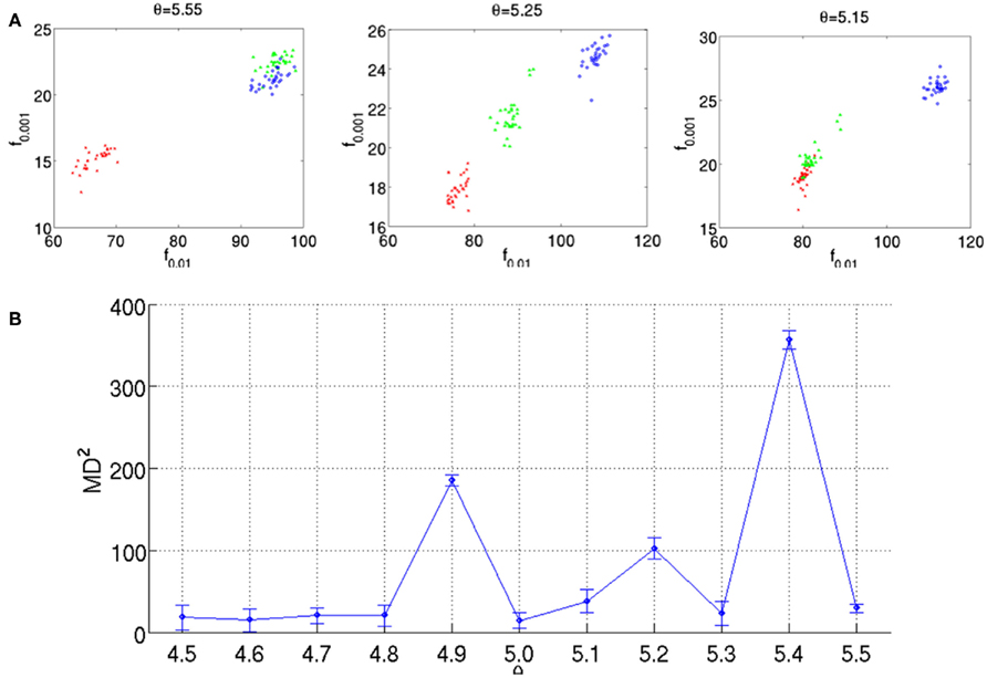
Figure 3. (A) Feature maps obtained for three operating temperatures as indicated by θ on each figure. The two features (i.e., axes) used in this representation are the transient features extracted from the response x₁ of TGS2600 and x₂ of TGS2610. Each of the analyte classes contain 10 samples, which are labeled with a different color/shape on the maps. (B) MD2(θ) evaluations estimated from the dataset for 11 heater voltages. Figure reprinted from Muezzinoglu et al. (2010), Copyright 2010, with permission from Elsevier Science.

Utilizing a similar statistical argument, Raman et al. (2009) pioneered the development of an optimization method to design micro-sensing arrays for complex chemical sensing tasks. The method consisted of utilizing statistical methods to systematically assess the analytical information obtained from the conductometric responses of chemo-resistive elements at different operating temperatures, i.e., the similarity/orthogonality of responses; test their reproducibility; and determine an optimal set of material compositions to be incorporated within an array of sensors for the recognition of individual species. They presented qualitative and quantitative approaches to determine both the sufficiency of the chosen materials for sensing targets in the test matrix and an optimal array configuration for the desired application.

In order to optimize the array configuration, the authors presented a modular approach, a sophisticated temperature pattern (see Figure 4A) and micro-hotplate platforms with different metal-oxide chemo-resistors (see Figure 4B) that examines the target matrix with five high-priority chemical hazards (i.e., ammonia, hydrogen cyanide, chlorine, ethylene oxide, and cyanogen chloride). The temperature program used to operate the sensing elements toggles the temperature between (a) 32 ramp values that sample most of the temperature range of the device and (b) four different baseline temperature values to allow relaxation toward some initial state prior to each ramp temperature. These different baselines allow thus different film–analyte interactions (i.e., adsorption/desorption, decomposition, and reaction) at the sensing surface prior to the ramp measurements. Then, they defined the following objective function with three components:

FIGURE 4

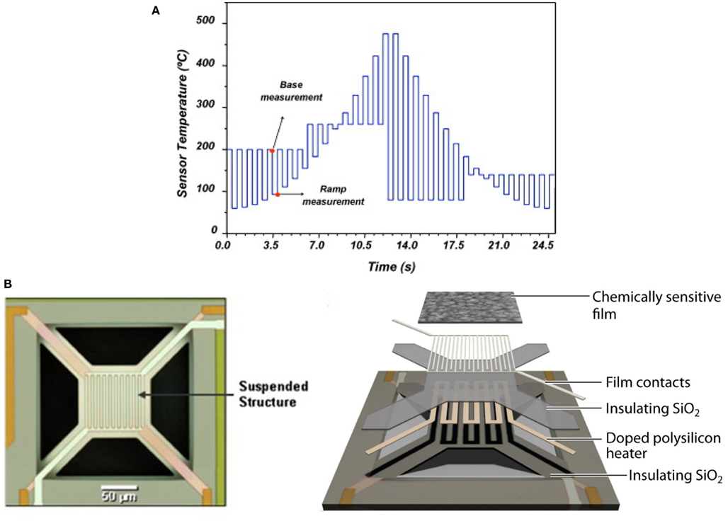
Figure 4. (A) Temperature program used for the detection of high-priority chemical hazards. A conductance measurement was made at each base and ramp temperature, but only the ramp values were used for further analysis in this study. (B) Micro-sensor array platform. A layered schematic showing the three primary components of the micro-sensor elements: polycrystalline silicon heater, interdigitated platinum electrodes, and metal-oxide sensing film. Figure reprinted from Raman et al. (2009), Copyright 2009, with permission from Elsevier Science.

where J is the maximization term that takes into account the sufficiency of solution (i.e., separability of the five chemical analyte clusters from different background conditions and from each other); N₁ and N₂ are two penalty terms that symbolize the number of different materials used and the array size respectively; and γ₁, γ₂, and γ₃, are component weights. The two penalty terms allow comparison between solutions with different numbers of materials and array sizes. In order to be able to increase the objective function, each new material or array element must increase the analyte’s cluster separability sufficiently to compensate for its “cost.” This cluster separability is derived from Fisher’s LDA as follows:

where S_W and S_B are the within-cluster and between-cluster scatter matrices, respectively. Being the ratio of the spread between classes relative to the spread within each class, the measure J increases monotonically as classes become increasingly more separable.

With this approach, the authors were able to demonstrate that cycling each sensing film through the 32 temperatures shown in Figure 4A did not necessarily create information that spanned 32 different dimensions. The responses were highly correlated and information seemed to be grouped based on temperature ranges; all lower temperature responses of a film type provided similar information that differs from that available from high temperature signals. On the other hand, cross-correlations computed across materials were comparatively lower than self-correlations. Therefore, taken together with the results from the dimensionality reduction analysis, these results suggested that different materials provide orthogonal information about the target analytes.

There is a last important remark to emphasize here. The form of dependence of the objective function of the methods presented here on their respective optimizable control parameters is initially unknown, yet to be inferred from a provided training set containing labeled measurements from the same sensor array at representative values of the parameter itself. As a consequence, any change in the problem setup, e.g., addition or removal of an analyte class, necessitates a re-calculation of the control parameter with the updated dataset, meaning that the sensor array must be re-conditioned for each class configuration. This outcome, nonetheless, is normal for any optimization solution considered, meaning that the found solution is to be customized to the set of analytes being analyzed. In any case, the statistical methods presented in this section provided a generalizable methodology for designing and evaluating array-based solutions for a wide variety of specific detection problems. Ultimately, it is envisage that the advances generated by these methods are critical to the production of pre-programmed micro-sensors for non-invasive, real time, multi-species recognition relevant to homeland security, and other applications involving trace analyte detection in complex chemical cocktails.

On the Optimization of Single Chemical Sensors

Much less attention has been paid to the optimization of metal-oxide sensors as a single device. As stated at the beginning of this review, and more specifically in Section “Metal-oxide Gas Sensors and Temperature Dependence,” there are an extensive number of articles reporting empirical studies dealing with dynamic features obtained from transient responses, e.g., different temperature waveforms patterns and stimulus frequencies implemented as a countermeasure to the effects of selectivity and reproducibility encountered in gas sensors. There is no doubt that a high variance in response is detrimental in most chemo-transduction applications that must be tackled. This general treatment, though, constitutes only one facet of the sensor optimization problem that does not necessarily yield better performance in the odor identification task. The reason for this is that a reduction in the response variance does not ensure a non-overlapping class configuration in the feature space. Therefore, to maximize classification performance, one needs a more comprehensive formulation that quantifies the separation of specific odor classes in the sensor response. Both of these aspects have been covered in literature under the notion of “optimization.” The thematic issues relevant to these works will be reviewed here.

Optimization of Excitation Profiles

Chemical sensing can benefit from a variable-temperature signal generation. In most of the cases, the temperature variation (a.k.a. temperature modulation) has been approached empirically by implementing various temperatures waveforms and stimulus frequencies (Sears et al., 1989a,b, 1990; Nakata et al., 1992, 1996, 1998; Semancik and Cavicchi, 1999). Although the results achieved by such a technique are very promising, in most of the reported works the selection of waveforms and the frequencies used to modulate sensor temperature has been conducted in a non-systematic way (Davis, 1991; Corcoran et al., 1998; Choi et al., 2002; Fort et al., 2002, 2003; Huang et al., 2003). Even the selection of features from the sensor transients is a somewhat obscure process. Therefore, since these selections are based on a trial and error procedure, there is no way to ensure that the modulation frequencies, modulation depth, or features chosen are the optimal for a given application. Very few authors, though, have systematically addressed this problem by suggesting different optimization strategies.

The first approach to review, in this context, is the one implemented by Kunt et al. (1998) and Cavicchi et al. (1996), who pioneered the development of an optimization method for temperature-modulated micro-hotplate gas-sensor devices. They implemented a two-step optimization process for determining the optimal temperature trajectory (or trajectories) that would exploit the information characteristics contained in the sensor dynamics when operated in temperature-pulsed mode. In particular, the authors sought to optimize the said sequence by adapting the pulse amplitude, pulse duration, delay between two consecutive pulses, and number of pulses in a cycle to better discriminate between two different gaseous analytes: ethanol and methanol. In the first stage, the authors introduced a black-box dynamical model of the sensor from input–output experimental data; they input a temperature programmed excitatory signal to the heating element of a single micro-hotplate sensor device and collected the sensor conductance in presence to vapors of methanol and ethanol. The authors then sought to predict the next conductance value of the sensor response (y_i+1) from the previous values of the conductance as well as the next and previous values of the temperature set points thus,

where n_y and n_u represent the model order in the input and output, respectively.

Utilizing different dynamic modeling methods, a suitable model F(·) was then built from the experimental data collected, being the wavelet network (WNET) method, for this particular case, the most accurate of all the tested methods. This initial model was further trained to set the final parameter values of the model F(·) and then used to simulate the sensor response to different temperature programs. In the second stage, the authors then implemented an off-line optimization routine to find the “optimal” temperature profile that maximizes the distance between the (simulated) temperature-modulated sensor responses to the targeted gases, thus

where y^MeOH and y^EtOH are the conductance responses predicted by the WNET models for methanol and ethanol, respectively.

Above, the search space for this optimal temperature profile is over a limited subset of realizable temperature pulses (e.g., lower and upper limits are chosen based on the sensor structure) and under the constraint that two consecutive pulses cannot differ in more than 40°C in order to avoid drastic changes in the surface. Finally, the metric used to quantify the said distance is the normalized sum of squared differences (NSSD) between the two response curves

where n is the number of temperature pulses in a cycle.

Figure 5 shows the optimal temperature profile to discriminate ethanol and methanol that was computed and validated through experimental measurements. This temperature profile (see the temperature profile shown in Figures 5C,D) produces methanol and ethanol responses that are out of phase (i.e., easy to discriminate). On the other hand, when applying a simple linear ramp (see Figures 5A,B), the sensor responses to ethanol and methanol were highly overlapped (i.e., becoming a non-trivial case of discrimination).

FIGURE 5

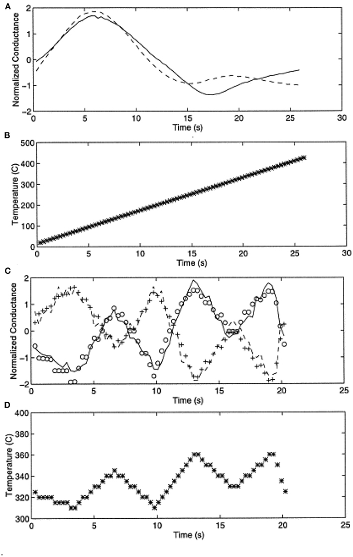
Figure 5. (A) Normalized conductance response to methanol (solid) and ethanol (dashed) upon applying a linear temperature ramp as shown in (B). (C) Actual experiments with methanol (solid line) and ethanol (dashed line) gases, model predictions are shown by circles for methanol and plus for ethanol models; (D) the optimum temperature profile derived from the off-line optimization process. Note the dramatic improvement in discrimination between (A) and (C). Figure reprinted from Kunt et al. (1998), Copyright 1998, with permission Elsevier Science.

Although this methodology is systematic and should be applicable to other analytes, its application to the qualitative and quantitative analysis of multi-component mixtures is not straightforward. The fact that the method relies on the construction of good predictive response models, complicates the optimization process for multi-gas, concentration variant environments.

With this motivation, more recently Vergara et al. (2005a,b, 2007a, 2008) introduced, in a series of works, a system-identification method for optimizing the temperature-modulation frequencies in order to solve a given gas analysis problem. The optimization method consisted of utilizing one of the most useful types of periodic signal for process identification, the pseudo-random sequences of maximum length (PRS-ML), either binary or multi-level, to determine the most suitable temperature-modulation frequencies for discriminating and/or quantifying a number of specific target compounds at different concentrations.

Pseudo-random sequence signals are the most popular choice for the persistently exciting perturbation signals required in system identification. The most common application of these sequences is the identification of linear systems. In particular, the pseudo-random signal sequences considered by the authors in their optimization scheme are based on maximum-length q-sequences, either binary or multi-level¹, the generation and properties of which were described by Zierler (1959). The relevant theory behind these signals is based on the algebra of finite fields. When q (the number of levels) is a prime, the digits of the sequence are the integers 0, 1, …, (q − 1) and the sequence can be generated by a q-level, n-stage shift register with feedback to the first stage consisting of the modulo q sum of the outputs of the other stages multiplied by coefficients a₁, …, a_n, which are also the integers 0, 1, …, (q − 1). The length (or period) of a maximum-length sequence is qⁿ − 1, which signifies that the sequence repeats itself after qⁿ − 1 logic values. The pseudo-random sequences are periodic, deterministic signals that have a flat power spectrum over a large frequency range. These properties imply that a PRS-ML shares some properties with white noise, but with the advantage of being repeatable, which makes these signals even more attractive and suitable for the system-identification task ahead. The generator of such a sequence and an example of a 5-level sequence (fragment) are shown in Figures 6A,B, respectively. Notice how the initial state of the shift register can be any combination of length n of the values 0, 1, …, (q − 1), with an exception made of n = zeros, and that each combination of these values appears as the state of the register exactly once during a period of the PRS-ML (Godfrey, 1993).

FIGURE 6

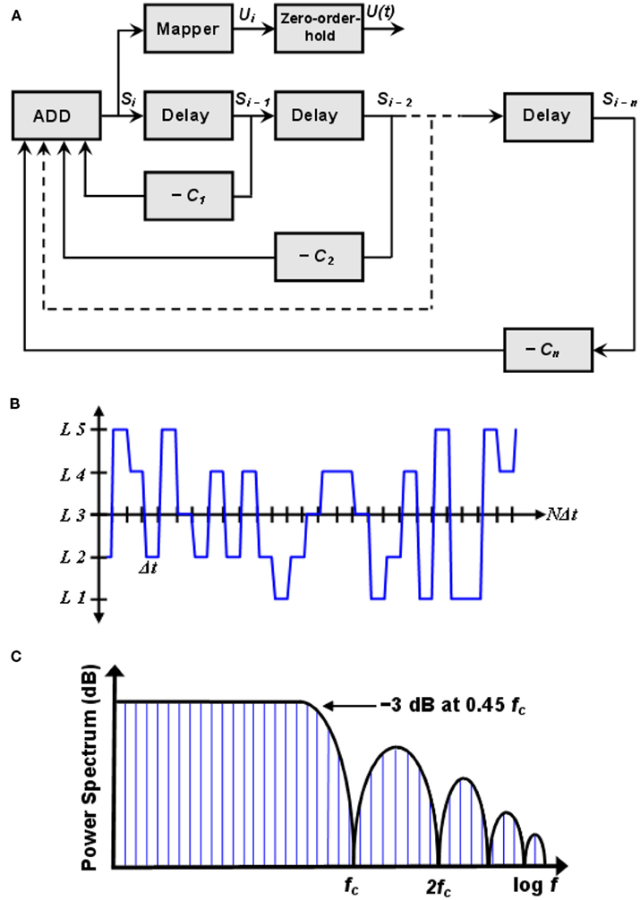
Figure 6. (A) A q-level pseudo-random maximum-length sequence generator. (B) Fragment of a 5-level pseudo-random sequence. (C) Discrete power spectrum of a PRS-ML signal. Spectral resolution is f_c/L, where f_c is the frequency of the clock signal applied to the shift register and L is the length of the sequence. Figure reprinted from Vergara et al. (2007a), Copyright 2007, with permission Elsevier Science.

The impulse response, h(t), is the main descriptor of a linear invariant system. Among the different strategies to estimate the impulse response, noise based methods allow to excite the system under study for enough time to supply it with the necessary energy to obtain a good estimate of h(t). By using white noise as excitation signals, one ensures that there is a homogeneous distribution of the energy over a large frequency range. Since PRS-ML signals have a low crest factor (i.e., low peak-to-average factor), they minimize the risk of saturating the system under study, which, in practice, means that these signals contain energy enough to obtain a good signal-to-noise ratio in a wide frequency range (i.e., measurement with high dynamic range) and that they avoid possible sensor non-linearities caused by signals with high crest factors (e.g., impulsive signals). Therefore, since these excitatory noise signals are deterministic, reproducible results are expected to be obtained, provided that the conditions of the system under analysis remain unchanged.

The power spectrum envelope of a PRS-ML is almost flat up to a frequency equal to 0.45 × f_c, where f_c is the frequency of the clock signal applied to the shift register used to generate the signal. The power spectrum is discrete and the separation between spectral lines (i.e., the spectral resolution) is f_c/L, where L is the length of the PRS-ML. Figure 6C shows the power spectrum of a PRS-ML signal, where, as observed, the power spectrum envelope is similar to the power spectrum of white noise up to the −3 dB cut-off frequency, which in this particular case is equal to 0.45 × f_c.

When the pseudo-random sequence is a maximum-length signal, the impulse response estimate, ĥ(n), can be obtained by computing the circular cross-correlation between the excitatory signal, x(n), and the response signal, y(n). The circular cross-correlation of two sequences x and y in Â^L may be defined as,

Above, the cross-correlation is circular since l + n is interpreted as modulo of L, where L is the length of the sequence and that can be optionally utilized as a normalization factor. The circular cross-correlation between the input and output sequences can readily be interpreted in terms of ĥ(n), since the autocorrelation function of the PRS-ML signal is of approximately impulsive form.

The whole optimization method proposed is illustrated in Figure 7. In a practical instance, it works as follows. First, a voltage PRS-ML signal is applied to the heating element of a micro-hotplate gas sensor while the sensors are exposed to various target compounds (e.g., nitrogen dioxide, ammonia, ethylene, ethanol, acetaldehyde, and their binary mixtures), hence ensuring that the sensor’s working temperature is modulated over the whole wide frequency range considered. Then, for each individual target compound the impulse response h(t) is computed as the circular cross-correlation between the excitation signal (PRS-ML) and the sensor response. Afterward, the absolute values of the FFT of the impulse response estimate are calculated, determining, in essence, which spectral components contain important information for the identification and quantification of gases. Finally, each individual frequency is ranked on the basis of its information content (between-class to within-class scatter ratio), and a subset of the most informative frequencies is selected. As the authors have shown in their results, this procedure succeeded in maximizing the discrimination and quantification of various gases and their mixtures using even a single sensor with its optimized set of modulating frequencies.

FIGURE 7

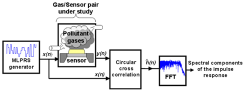
Figure 7. Study of the sensor/gas system using MLPRS signals. The MLPRS voltage signal, x(n), is input to the heating element of a micro-hotplate gas sensor. The transient of the sensor conductance (i.e., the response in the presence of gases), y(n), is recorded. An estimate of the impulse response, ĥ(n), can be computed via the circular cross-correlation of x(n) and y(n). Finally, by performing the FFT of ĥ(n), the spectral components of the impulse response estimate are found. Figure reprinted from Vergara et al. (2007a,c), Copyright 2007, with permission Elsevier Science.

In addition, the authors extended their optimization study on a completely two-stage validation procedure, demonstrating thus the consistency and robustness of the method itself (Vergara et al., 2007c, 2008). The two-stage method consisted of, first, running the whole optimization process presented above utilizing a set of measurements pre-recorded with one micro-sensor array, and then, validate the resulting outcome employing a new set of measurements collected with a different sensor array with the same characteristics of the one used in the first stage. This new set of measurements, though, was based on the multi-sinusoidal temperature-modulating signal showed in Figure 8A, the frequencies of which were the reduced set of the optimal ones estimated in the first stage. The Figures 8B,C show the FFT spectra of the transient response of a sensor in the presence of two different analytes [acetaldehyde (50 ppm) and ethylene (50 ppm)]. Notice how the peaks in these plots correspond to the “optimal” temperature-modulating frequencies selected. As the variation of peaks’ height (i.e., the pattern) between Figures 8B and 8C shows, significant improvements in the classification and quantification capability of a single gas-sensor operated under the temperature-modulation scheme is attained. Particularly, their results revealed a classification performance of up to 98.2% even when a single sensor was used, and a shift of the odor concentration prediction of down to 0.92 ppm for single species and 2.81 ppm for binary mixtures. These illustrated performance improvements were expected, though, in the sense that, as the Figures 8B,C shows, a different pattern develops when different odorant species are measured, whilst the resulting pattern is preserved, to a large extent, when the vapor concentrations change, meaning that the illustrated evaluation is a reliable indicator of the improvement of the classification capability of the sensors when their operating temperature is modulated at the frequencies selected.

FIGURE 8

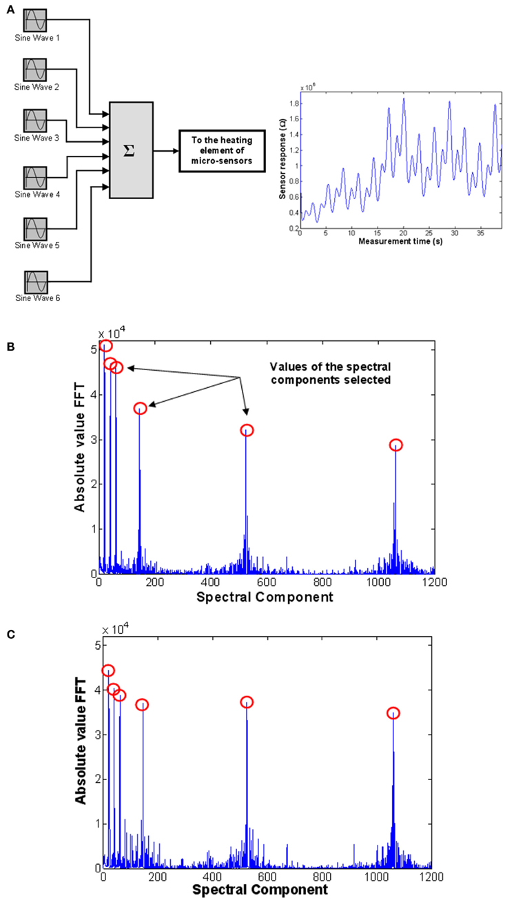
Figure 8. (A) Setup used to generate a multi-sinusoidal signal, which consists of the sum of six sinusoids of identical amplitudes and different frequencies. The signal is applied to the heating element of the micro-sensors studied. FFT (absolute value) of the transient response of a temperature-modulated WO₃ micro-hotplate sensor in the presence of (B) 50 ppm acetaldehyde and (C) 50 ppm ethylene. Figure reprinted from Vergara et al. (2007a, 2008), Copyright 2007 and 87, Copyright 2008, with permission Elsevier Science.

As a final remark to emphasize here, it was demonstrated that for each gas-sensor pair, the modulating frequencies selected are related to the characterization of the interaction between the metal-oxide layer and the gas, e.g., film microstructure; surface diffusion; and reaction kinetics. Even though the method was implemented for the analysis of the specific qualitative and quantitative task earlier described, this optimization procedure is generic and could be applied to many qualitative and quantitative gas analysis applications.

Optimization of the Operating Temperature: Internally Tuning the Chemical Sensors

It has long been known that varying or setting different values of the sensor’s operating temperature affects all the aspects of the sensor response, including its selectivity and sensitivity to different volatile compounds (i.e., the sensor’s ability to encode the odor information), as well as its reproducibility. For example, carbon monoxide (CO) is usually best detected at lower operation temperatures (e.g., 250°C) when using a tin dioxide based sensitive layer, whereas higher temperatures (e.g., 350°C) are used for monitoring hydrocarbons such as methane among others. In view of this, different strategies, such as the idea of periodically changing the sensor working temperature, have been implemented to maximize the performance of the sensors. However, despite the promising results obtained in all these previously cited attempts, one question remains unanswered: given a metal-oxide based chemical sensor, how does one select the best (i.e., the optimal) operating temperature (or temperatures) for fast and reliable discrimination or quantification of chemical species? One conceivable manner to address this issue is to empirically vary the operating temperature through all the possible values available in the sensor so that its response to each gas is maximized (Cavicchi et al., 1996; Maziarz and Pisarkiewicz, 2008). However, this may be an expensive and inefficient solution because it does not guarantee the improvement of the performance of the sensors.

Undoubtedly, heightened sensitivity to a spectrum of chemical hazards is necessary for the detection of analytes at relevant concentrations. However, this general treatment constitutes only one facet of the problem, a substantial selectivity is also necessary to rapidly and accurately perform the odor identity representation task. The reason for this is that an increase in the response does not ensure a non-overlapping class configuration in the feature space. Therefore, to maximize the classification performance, one needs a more comprehensive formulation that quantifies the separation of specific odor classes in the sensor response.

Following this scheme, Vergara et al. (2009b, 2010) formulated an optimization method to select, for a single sensor, the best operating temperature to discriminate a given set of odorants. The authors presented a rigorous way of selecting the best operating temperature for a chemical sensor. The method hinges on an information measure widely used in information theory, namely the relative entropy or Kullback–Leibler divergence (KL-divergence; Kullback and Leibler, 1951), a measure index that rates the difference between two probability distributions. Since these probability distributions may belong to one of the disjoint classes of interest in a particular odor universe, this annotated quantitative measure shows how odors are encoded in every odorant chemo-receptor and how distinguishable they are from each other at different parameter values. Tuning a control parameter, such as the sensor’s operating temperature, will maximize such a difference, yielding thereby a substantial improvement in the classification performance (separation of classes) and reproducibility of the process. In particular, using a metal-oxide gas sensor in an odor-discrimination instance, the authors demonstrated the proposed criterion by studying the impact of adjusting the sensing parameter on the odor-sensor pair interaction and on the confidence of the information yielded by the sensor individually.

The KL-divergence is a very well-known index for class separation that is a non-commutative measure (a “distance” in a heuristic sense) of the difference between two distributions: a conceptual reality [probability distribution g(·)] and an approximate model [probability distribution h(·)]. For two continuous functions qualifying as probability distributions, the KL-divergence is defined by the integral:

where KL is the measure of “information” lost when a model h(·) is used to approximate reality [i.e., model g(·); Kullback and Leibler, 1951].

The utility of the KL-divergence is based on a certain number of properties that make it unique for measuring the difference between two probability distributions. For example, this approach can account for a number of key characteristics of a response, including, for example, higher order moments (e.g., skewness) or multi-modality, which in turn may be involved in the response distribution (at least in odor representation), causing thus loss of information. However, the measure is still not commutative, i.e., KL(g(x) || h(x)) is in general different from KL(h(x) || g(x)); therefore, the KL-divergence is not a legitimate metric by itself. As a consequence, a symmetrized version, namely the KL-distance, can be readily composed after a straightforward manipulation given by:

which the authors adopted as a measure of the class-conditional distributions’ separation for the specific purpose.

In a context C (i.e., the likelihood of occurrence of each odor stimulus from a finite list of analytes whose classes are known) in which one is trying to discriminate two compounds that is complicated by the similarities/overlaps among the class-conditional distributions, the KL-distance index, given in Eq. 16, constitutes an accurate measure of discrimination, hence a good indicator of the classification performance for any unbiased classifier. Therefore, given the simplest two-dimension discrimination problem (i.e., a two-class discrimination task), when the class-conditional distributions depend on a measurement parameter (e.g., operating temperature in metal-oxide gas sensors), maximizing the KL-distance is a valid objective function for tuning that parameter (see Figure 9).

FIGURE 9

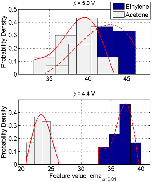
Figure 9. Class-conditional probability distributions in a two-class discrimination instance. Each class response models the histograms by a normalized fifth-order polynomial (plain and dashed lines). These models accurately approximate the sensor’s response to an odor class while accounting for the asymmetry (i.e., skewness) in the distribution. The KL-distance index then captures the influence of the operating parameter on the separability of such distributions. Maximizing this index for a pair of distributions results in a better discrimination between the corresponding two classes (top versus bottom figures). Figure reprinted from Vergara et al. (2010), Copyright 2010, with permission Elsevier Science.

Using a binary classification instance as a case of study may be very convenient from many perspectives; in odor representation, however, this assumption may be very unrealistic. When the number of classes (i.e., the possible outcomes of the identification problem) is more than two, the KL-distance should be generalized to promote the dispersion of the whole classes. The authors have addressed this issue by replacing (16) with the sum of pair-wise distances, thus:

where |C| denotes the number of classes in the problem and g_i(·) and h(·), i ∈ C, j ∈ C, are the class-conditional distributions, each potentially depending on the operating parameter (e.g., the sensor’s operating temperature). The CKL quantifies the difficulty of the classification problem. When this quantity is large, an arbitrary classifier is expected to perform with higher accuracy, since, relative to a small CKL, the distribution within each class shrinks whilst the distance among the considered classes increases in the feature space.

Assuming that β denotes an intrinsic parameter of a sensor device that alters the response characteristics (see Figure 9), then the problem configuration CKL is expected to be sensitive toβ itself. Hence, the value

defines an optimum operating condition for the classification problem at hand.

In demonstrating their optimization scheme, the authors applied the criterion (18) to optimize the operating conditions of commercialized metal-oxide gas sensors (sensors provided by Figaro Engineering Inc., Japan, http://www.figaro.co.jp). In particular, they have examined the performance of each gas sensor in a six-class classification problem, comprised by six different analytes dosed at different concentrations (i.e., ethylene, ethanol, and toluene dosed at 10 ppm; acetone and acetaldehyde at 100 ppm; and ammonia at 120 ppm). They thus studied the impact of adjusting its sensing parameter β on the odor-sensor pair interaction and on the confidence of the information yielded by the sensor individually.

In principle almost any controllable variable that alter or modify the operating characteristics of the sensor, such as the environment temperature, flow rate, or even construction methodologies, can be used as a parameter of the response profile that can be tuned to improve the processing performance. However, in this popular odor sensing technology, it is very well-known, and proved in many empirical works (see, e.g., works from Sears and Nakata), that there is a strict dependence of the sensor response on its operating temperature (temperature normally ranging in high orders of magnitude, e.g., 400°C, responsible of the adsorption/desorption reaction occurring at the micro-porous surface of the sensor in response to an analyte). Accordingly, having such an easy way of interacting with the sensor, the most natural way to optimize the sensor device is with respect to this parameter (i.e., the sensor’s operating temperature), assuming that all the other parameters remain constant. Since the sensor packaging does not permit direct access to this temperature, its tuning can be achieved via a resistive heater element with controllable voltage, which has a deterministic one-to-one mapping with the actual active layer temperature². Accordingly, the authors have considered this heater voltage and the operating temperature interchangeably as the sensing conditioning parameter β to be optimized.

To demonstrate the optimization scheme in a practical instance, the authors established the following procedure: Initially, the form of the dependence of CKL on β is initially unknown, yet to be inferred from a provided training set (containing labeled measurements) from the same sensor at representative β values. For each sensor the authors then compiled a comprehensive dataset containing the analytes described above. Each set of time series contained 30 independent measurements taken from each class at each of the 13 sensor operating temperatures corresponding to the heater voltages β ∈ {3.8, 4.0, …, 6.2 V}³. Thus, the authors represented each of the chemo-sensory records, associated with each odor class and operating temperature, as independent and identically distributed (i.i.d.) samples, from which the class-conditional distribution is derived. Then, they modeled each odorant class by a polynomial fit to the histogram of previously collected samples from that odorant type. In particular, they consider a fifth-order polynomial to represent odorant class/histogram relation. Finally, by plugging these functions into Eq. 17, the CKL criterion (18) was implemented, and the maximum β value obtained, yielding thus the optimal operating temperature values for the particular discrimination task. As a measure of separability, the evaluation of the CKL for the six classes at each temperature β yielded the profile shown in Figure 10 (dashed lines). Based on this evaluation, the best operating condition for each sensor to distinguish between the set of classes is determined by the maximum value of their respective curves.

FIGURE 10

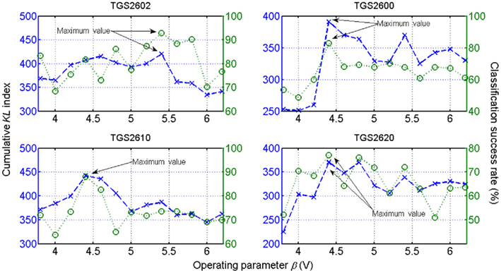
Figure 10. Observed discrimination performance of a linear-SVM classifier of each sensor on the six-class identification problem (dotted lines). Profiles for each sensor as estimated by the CKL index (dashed lines) with respect to β. Based on the proposed criterion, the optimal operating condition that best discriminates between the set of classes can be determined for each sensor individually by obtaining the maximum value of the curve shown. Figure reprinted from Vergara et al. (2010), Copyright 2010, with permission Elsevier Science.

To demonstrate the consistency and robustness of the optimization method, the authors conducted a validation process that consisted of measuring the correlation between the information given by the optimization criterion (18) and the performance given by an arbitrary linear support-vector classifier based classifier. As observed in Figure 10, the results yielded by the SVM classifier (see Figure 10, dotted lines) follow a similar pattern to the estimated measure CKL index (Figure 10, dashed lines) in the sense that their extreme points occur at the same β values. The ordering of these points in magnitude was also preserved to a large extent, meaning that the proposed measurement is a reliable indicator of the classification performance at almost all temperatures within the range.

In addition, the authors validated the whole optimization process with the second dataset 4 months later. To validate the results, they re-calculated the proposed cost function CKL of the second dataset by applying the same procedure described above. Based on this re-evaluation, the best operating condition to distinguish between the new set of classes was determined, and compared to the performance yielded by the linear-SVM classifier. As can be seen in Table 1, the results obtained in the validation stage perfectly matches with the information given by the classifier, showing the consistency of the method. These results indicate that the proposed CKL measure-index is optimum for any complexity of probability distribution models; hence, for any type and number of odorants as well as any type of sensor technology with a conditioning parameter, provided that these models are accurate in identifying the response distribution. Nevertheless, the method could be extended to an arbitrary classification instance as needed, including complex odors at different concentrations or mixtures of gases, provided that a sufficiently representative database of relevant measurements is available. It is also important to emphasize that the solution β* does not impose a particular classification method. Therefore, the parameter value resulting from the maximization of Eq. 18 simplifies the task of an arbitrary unbiased classifier.

TABLE 1

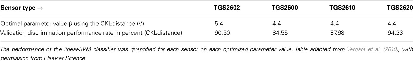
Table 1. Optimal operating parameter values β selected versus the observed classification performances for each metal-oxide gas sensor given by the linear-SVM classifier during the validation stage.

It is important to comment on one last issue here. An operating condition is optimal for a well-defined task. If this task changes then the best condition should be re-calculated. This applies, nonetheless, to any optimization method, not just this one. For example, considering a generic classifier training instance, if the training data changes (e.g., some data turns out to be invalid or relabeled), then the device needs to be re-trained in order to determine the optimal performance. In this optimization case, a re-calculation of β* with the updated dataset is therefore needed, too.

Active-Sensing Optimization

The idea of applying sophisticated signal processing procedures and optimization strategies to ameliorate the performance of metal-oxide gas sensors has been around for more than two decades. Researchers have since used a wide array of dynamic features obtained from transient responses, but most of these studies have been empirical. To the best of our knowledge, very few studies have proposed systematic approaches to optimizing the sensor performance as a single device (Cavicchi et al., 1996; Kunt et al., 1998; Vergara et al., 2005a,b, 2007a,c, 2008, 2009a,b, 2010). These methods, though, require that the optimization be performed off-line; therefore, they cannot adapt to changes in the environment. In view of this, a novel active-sensing approach that can optimize the temperature profile online (i.e., as the sensor collects data from its environment), has recently emerged in literature. The most relevant works on this thematic issue are reviewed in this section.

Active-sensing strategies are inspired by the fact that perception is not a passive process (Gibson, 1979), but an active one, in which an organism controls its sensory organs in order to extract behaviorally relevant information from the environment (see Figure 11A). Active sensing has been traditionally used in robotics and computer vision, in which the localization and navigation tasks, on the one hand, and the recognition of three-dimensional (3-D) objects from 2-D image, on the other hand, respectively, is a recurrent theme (Paletta and Pinz, 2000; Denzler and Brown, 2002; Floreano et al., 2004). In chemical sensing, however, it has received only minimal attention. In one of the earliest studies, Nakamoto et al. (1995) developed a method for active odor blending, where the goal was to reproduce an odor blend by creating a mixture from its individual components. The authors developed a control algorithm that adjusted the mixture ratio, so the response of a gas-sensor array to the mixture could matched the response to the odor blend.

FIGURE 11

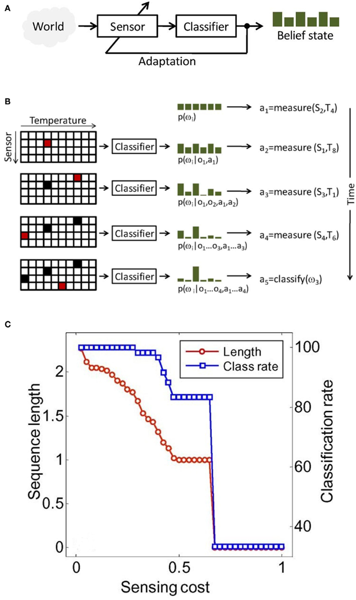
Figure 11. (A) In active sensing, the system adapts its sensing parameters based on its belief about the world (e.g., class membership of a stimulus). (B) Illustration of active-classification with an array of four metal-oxide gas sensors, 10 temperatures per sensor, and a discrimination problem with six chemicals. At time zero, no information is available except that classes are a priori equiprobable: p(ω⁽ⁱ⁾ = 1/6). Based on this information, the active classifier decides to measure the response of sensor S2 at temperature T4, which leads to observation o₁ and an updated posterior p(ω⁽ⁱ⁾|o₁,a₁). After four sensing actions, evidence accumulated in the posterior p(ω⁽ⁱ⁾|o₁… o₁, a₁… a₁) and the cost of additional measurements are sufficient for the algorithm to assign the unknown sample to class ω (3). In this toy example, accurate classification is reached using only 10% of all sensor configurations. (C) Classification performance and average sequence length as a function of feature acquisition costs. Figure adapted from Gosangi and Gutierrez-Osuna (2009) © IEEE.

It was not until 2010, when Gosangi and Gutierrez-Osuna(2009, 2010) proposed an active-sensing approach to optimize the temperature profile of metal oxide sensors in real time, as the sensor reacts to its environment. To see how their approach works let us consider the problem of classifying an unknown gas sample into one of M known categories {ω⁽¹⁾, ω⁽²⁾, …, ω^(M)} using a MOX sensor with D different operating temperatures {ρ⁽¹⁾, ρ⁽²⁾, …, ρ^(D)}. To solve this sensing problem, one typically measures the sensor’s response at each of the D temperatures and then analyzes the complete feature vector x = [χ¹, χ², …, χ^D]^T with a pattern-recognition algorithm. Although straightforward, this passive sensing approach is unlikely to be cost effective because only a fraction of the measurements are generally necessary to classify the chemical sample. Instead, the authors seek to determine an optimal sequence of actions a = [a₁, a₂, …, a_T], where each action corresponds to setting the sensor to one of the D possible temperatures or terminating the process by assigning the sample to one of the M chemical classes. More importantly, they seek to select this sequence of actions dynamically on the basis of accumulating evidence. This process is illustrated in Figure 11B.

In demonstrating their approach, the authors first model the sensor’s steady-state response at temperature ρ_i to chemical ω^(c) with a Gaussian mixture:

where M_i is the number of Gaussians, and are the mixing coefficient, mean vector, and covariance matrix of each Gaussian for class ω^(c), respectively. Given a sequence of actions [a₁, a₂, …, a_T], the authors assumed that the sensor progresses through a series of states s = [s₁, s₂, …, s_T] to produce an observation sequence o = [o₁, o₂, …, o_T]. Each state s_i represents a Gaussian in (19) and is therefore hidden. Following this step, they modeled the dynamic response of a sensor to a sequence of temperature pulses by means of an input–output hidden Markov model. This is a machine learning technique that can be used to learn a dynamic mapping between two data streams: (a) an input (temperature in this case) and (b) an output (sensor conductance). Once a dynamic sensor model has been learned, they then approach the temperature-optimization process as one of sequential decision-making steps under uncertainty, where the goal is to balance the cost of applying additional temperature pulses against the risk of classifying the chemical analyte on the basis of the available information. As a result, the problem is solved through a partially observable Markov decision process (Papadimitriou and Tsitsiklis, 1987).

Simulation results from this study are shown in Figure 11C; these results indicate that the method can balance sensing costs and classification accuracy: higher classification rates can be achieved by decreasing sensing costs, which in turns increases the length of the temperature sequence and the amount of information available to the classifier. One last think to comment on here is that the active-sensing approach proposed here has great potential in pioneering new strategies to be implemented in energy-aware chemical sensing networks using low-cost commercial sensors.

Conclusion and Outlook

Most of the work reviewed in this article has focused on optimization schemes for single sensors or sensor arrays within a single chemo-sensing system. Advances at the intersection of materials science, micro- and nano-technology, microelectronics, and chemical micro-sensory systems together with the explosion of mobile computing and the wireless communications capabilities will soon dramatically influence the deployment of massively distributed sensory micro-systems networks with capabilities that, only years ago, were confined to the lab bench of research laboratories. It can be concluded from the contents of this review that the integration of chemical micro-systems and wireless networks may, indeed, have a profound impact not only in different applications ranging from environmental monitoring to personal health care, but also in the formidable challenges present at the current practices of sensor management and data analysis. However, we believe that the sensor-based detection of chemical analytes in a dynamic real-world environment is a complex task, in which the interest of the final-user is to have reliable, user-friendly, and affordable sensory systems, irrespective of the internal system complexity. Therefore, the concept of an adaptive optimal sensory system can be most successful.

Adaptive sensory systems may be devices that include various chemical transducer types and sensor operation modes, the use of auxiliary sensors, and separation and pre-concentration units, which can respond or adapt their optimal operation to the occurring analysis situations or events. Then, in the instance where a certain odorant compound or a major interfering chemical is present, the sensor/feature selection, sensor operation mode, feature extraction, and data treatment should be able to adapt to this event so that their protocols execute in such a way that the best-possible target-analyte detection is achieved or that the influence of the interfering analyte can be recognized and minimized if not suppressed at all. In dealing with the just described issues, it may be very effective to purposefully select or deselect sensors, to find the optimal sensor’s operation mode, or to use signal ratios or differential values instead of merely increasing the array size or the transducer diversity.

Another important observation to make from the optimization schemes reviewed here is that the chances for these optimization schemes to succeed, or in other words maximizing the performance in a gas-sensor identification system to be more precise, truly depends on multiple factors that all together determine the problem setup. These factors include the hierarchical level of the classification problem pursued (e.g., gas discrimination versus quantification and prediction of the gas concentration), the environmental parameter conditions, the features selected for evaluation, and the classifiers utilized to map the extracted features to class labels (Vergara et al., 2009a). A more comprehensive formulation addressing all of these options would almost certainly yield a better performance than the generic solutions presented in these works (Di Natale et al., 1995; Wilson and De Weerth, 1995; Martinelli et al., 2003; Vergara et al., 2007b,d). We held this issue, though, as an arguable position that we would address in future works.

Finally, when facing a general problem of sensor-array optimization, sensor selection, or sensor optimization, it would be worth considering the following steps:

1. In case there is domain knowledge (e.g., underlying physicochemical phenomena is known or a sensor response model is available), then consider building a better set of “ad hoc” features.

2. Are features commensurate? If a hybrid multi-sensor system is employed, which combines different odor sensing technologies it is likely that feature normalization will be of help.

3. If there is a need to prune the number of sensors or input features (e.g., for simplicity, data understanding, etc.) then start by assessing features individually. This will help in understanding their relative influence on the system. Additionally, if their number is too large use a variable ranking method to implement a first step of filtering.

4. In case some response patterns within the optimization database are suspected to be meaningless or have the wrong class labels, outliers should be detected by employing the top ranking features/sensors obtained in step 3.

5. In case there is not an evident option for the classifier model to be used, start by trying first a linear model. Following the ranking of step 3, construct a sequence of classifiers of similar nature using increasing (or decreasing) subsets of features (e.g., by implementing a forward or backward selection strategy). In case performance is matched or improved with a smaller subset, then try a non-linear classifier model with this subset. As a rule of thumb, it is better to try simple strategies first.

6. If the database available has a large number of samples and there is time enough and computational resources, then it is worth comparing several sensor/feature selection methods coupled to linear or non-linear classifier models. Consider combining filters either with wrapper or embedded approaches. Do not refrain from trying your own ideas.

7. Finally, in order to achieve a stable solution to the optimization problem and effectively improve performance, employ data re-sampling methods (e.g., by constructing bootstrap sets) and redo the sensor selection analysis for different sets.

Conflict of Interest Statement

The authors declare that the research was conducted in the absence of any commercial or financial relationships that could be construed as a potential conflict of interest.

Acknowledgments

This work was partially funded by NATO under the Science for Peace Program grant number CBP.MD.CLG 983914. A. Vergara is funded by the U.S. Office of Naval Research (ONR), contract number N00014-07-1-0741 and by the US Army Medical Research and Materiel Command and the United States Army Research Institute of Environmental Medicine (USARIEM), contract number W81XWH-10-C-0040 in collaboration with Elintrix Inc. E. Llobet is supported by the Spanish Ministry of Science and Innovation and the Catalan Agency for Research under the grant numbers TEC 2009-07107 and 2009-SGR-789, respectively. The authors also acknowledge Joanna Zytkowicz for reading and revising the manuscript.

Footnotes

1. ^One of the main reasons for considering signals with more than 2 levels is that multi-level signals provide the possibility of identifying a better estimate of the linear dynamics of a process with non-linearity than the binary sequences and that they can also be of use in the identification of the non-linear characteristics themselves (Vergara et al., 2005b, 2007a).
2. ^A look-up table with a deterministic one-to-one mapping of the actual active layer temperature and the controllable heater voltage was provided in Figaro Engineering Inc., Japan, http://www.figaro.co.jp
3. ^The operating temperature values selected perform a dataset with a temperature resolution (i.e., separation value among the temperatures evaluated) of 20°C, under the assumption that this temperature resolution suffices in making a reliable inference of the dependence of the CKL on the parameter value β.

References

Alkasab, T. K., White, J., and Kauer, J. S. (2002). A computational system for simulating and analyzing arrays of biological and artificial chemical sensors. Chem. Senses 27, 261–275.

Pubmed Abstract | Pubmed Full Text | CrossRef Full Text

Bhandawat, V., Olsen, S. R., Gouwens, N. W., Schlief, M. L., and Wilson, R. I. (2007). Sensory processing in the Drosphila antennal lobe increases reliability and separability of ensemble odor representations. Nat. Neurosci. 10, 1474–1482.

Pubmed Abstract | Pubmed Full Text | CrossRef Full Text

Barsan, N., Schweizer-Berberich, M., and Göpel, W. (1999). Fundamental and practical aspects in the design of nanoscaled SnO2 gas sensors: a status report. Fresenius J. Anal. Chem. 365, 287–304.

CrossRef Full Text

Cavicchi, R. E., Suehle, J. S., Kreider, K. G., Gaitan, M., and Chaparala, P. (1996). Optimized temperature-pulse sequences for the enhancement of chemically specific response patterns from micro-hotplates gas sensors. Sens. Actuators B Chem. 33, 142–146.

CrossRef Full Text

Choi, N. H., Shim, C. H., Song, K. D., Lee, D. S., Huh, J. S., and Lee, D. D. (2002). Classification of workplace gases using temperature modulation and two SnO2 sensing films on substrate. Sens. Actuators B Chem. 86, 251–258.

CrossRef Full Text

Clifford, P. K., and Tuma, D. T. (1983). Characteristics of semiconductor gas sensor II, Transient response to temperature change. Sens. Actuators B Chem. 3, 233–254.

Comini, E., Baratto, C., Faglia, G., Ferroni, M., Vomiero, A., and Sberveglieri, G. (2009). Quasi-one dimensional metal oxide semiconductors: preparation, characterization and application as chemical sensors. Prog. Mat. Sci. 54, 1–67.

CrossRef Full Text

Corcoran, P., Lowery, P., and Anglesea, J. (1998). Optimal configuration of a thermally cycled gas sensor array with neural network pattern recognition. Sens. Actuators B Chem. 48, 448–455.

CrossRef Full Text

Davis, L. (1991). The Handbook of Genetic Algorithms. New York, NY: Van Nostrand Reinhold.

Denzler, J., and Brown, C. M. (2002). Information theoretic sensor data selection for active object recognition and state estimation. IEEE Trans. Pattern Anal. Mach. Intell. 24, 145–157.

CrossRef Full Text

Di Natale, C., Marco, S., Davide, F., and D’Amico, A. (1995). Sensor array calibration time reduction by dynamic modeling. Sens. Actuators B Chem. 24, 578–583.

CrossRef Full Text

Dickinson, T. A., White, J., Kauer, J. S., and Walt, D. R. (1996). A chemical-detecting system based on a cross-reactive optical sensor array. Nature 382, 697–700.

Pubmed Abstract | Pubmed Full Text | CrossRef Full Text

Eklöv, T., Mårtensson, P., and Lundström, I. (1997). Enhanced selectivity of MOSFET gas sensors by systematical analysis of transient parameters. Anal. Chim. Acta 353, 291–300.

CrossRef Full Text

Floreano, D., Kato, T., Marocco, D., and Sauser, E. (2004). Coevolution of active vision and feature selection. Biol. Cybern. 90, 218–228.

Pubmed Abstract | Pubmed Full Text | CrossRef Full Text

Fort, A., Gregorkiewitz, M., Machetti, M., Rocchi, S., Serrano, B., Tondi, L., Ulivieri, N., Vignoli, V., Faglia, G., and Comini, E. (2002). Selectivity enhancement of SnO2 sensors by means of operating temperature modulation. Thin Solid Films 418, 2–8.

CrossRef Full Text

Fort, A., Machetti, M., Rocchi, S., Serrano, B., Tondi, L., Ulivieri, N., Vignoli, V., and Sberveglieri, G. (2003). Tin oxide gas sensing: comparison among different measurement techniques for gas mixture classification. IEEE Trans. Instrum. Meas. 52, 921–926.

CrossRef Full Text

Franke, M. E., Koplin, T. J., and Simon, U. (2006). Metal and metal oxide nanoparticles in chemiresistors: does the nanoscale matter? Small 2, 36–50.

Pubmed Abstract | Pubmed Full Text | CrossRef Full Text

Freund, M. S., and Lewis, N. S. (1995). A chemically diverse, conducting polymer-based “electronic nose”. Proc. Natl. Acad. Sci. U.S.A. 92, 2652–2656.

Pubmed Abstract | Pubmed Full Text | CrossRef Full Text

Gardner, J. W., and Bartlett, P. N. (1996). Performance definition and standardization of electronic noses. Sens. Actuators B Chem. 33, 60–67.

CrossRef Full Text

Gardner, J. W., and Bartlett, P. N. (1999). In Electronic Noses: Principles and Applications. Oxford: Oxford University Press.

Gibson, J. J. (1979). The Ecological Approach to Visual Perception. Boston: Houghton Mifflin.

Godfrey, K. (1993). Perturbation Signals for System Identification. Prentice Hall International, 39–49, 181–187, 321–347.

Göpel, W. (1985). Chemisorption and charge transfer at ionic semiconductor surfaces: VCH implications in designing gas sensors. Prog. Surf. Sci. 20, 1, 9–103.

CrossRef Full Text

Göpel, W. (1988). Chemical imaging I: concepts and visions for electronic and bioelectronic noses. Sens. Actuators B Chem. 52, 125–142.

CrossRef Full Text

Göpel, W., Hesse, J., and Zemel, J. N. (eds). (1991). Sensors, A Comprehensive Survey, Vol. 2. Weinheim: VCH.

Gosangi, R., and Gutierrez-Osuna, R. (2009). “Active chemical sensing with partially observable Markov decision processes,” in Proceedings of International Symposium on Olfaction and Electronic Noses (ISOEN 2009), Brescia.

Gosangi, R., and Gutierrez-Osuna, R. (2010). Active temperature programming for metal-oxide chemoresistors. IEEE Sens. J. 10, 1075–1082.

CrossRef Full Text

Gurlo, A. (2010). Nanosensors: does crystal shape matter? Small 6, 2077–2079.

Pubmed Abstract | Pubmed Full Text | CrossRef Full Text

Gutierrez-Osuna, R., Nagle, H. T., and Schiffman, S. S. (1999). Transient response analysis of an electronic nose using multi-exponential models. Sens. Actuators B Chem. 61, 170–182.

CrossRef Full Text

Guyon, I., and Elisseeff, A. (2003). An introduction to variable and feature selection. J. Mach. Learn. Res. 3, 1157–1182.

Huang, X., Liu, J., Shao, D., Pi, Z., and Yu, Z. (2003). Rectangular mode of operation for detecting pesticide residue by using a single SnO2 based gas sensor. Sens. Actuators B Chem. 96, 630–635.

CrossRef Full Text

Kullback, S., and Leibler, R. A. (1951). On information and sufficiency. Ann. Math. Stat. 22, 1, 79–86.

CrossRef Full Text

Kunt, T. A., McAvoy, T. J., Cavicchi, R. E., and Semancik, S. (1998). Optimization of temperature programmed sensing for gas identification using micro-hotplate sensors. Sens. Actuators B Chem. 53, 24–43.

CrossRef Full Text

Martinelli, E., Falconi, C., D’Amico, A., and Di Natale, C. (2003). Feature extraction of chemical sensors in phase space. Sens. Actuators B Chem. 95, 132–139.

CrossRef Full Text

Maziarz, W., and Pisarkiewicz, T. (2008). Gas sensors in a dynamic operation mode. Meas. Sci. Technol. 19, 055205.

CrossRef Full Text

Moseley, P. T., and Tofield, B. C. (eds). (1987). Solid-state Gas Sensors. The Adam Hilger Series on Sensors, Bristol.

Muezzinoglu, M., Vergara, A., Huerta, R., and Rabinovich, M. (2010). A sensor conditioning principle for odor identification. Sens. Actuators B Chem. 146, 472–476.

CrossRef Full Text

Muezzinoglu, M., Vergara, A., Huerta, R., Rulkov, N., Rabinovich, M., Selverston, A., and Abarbanel, H. (2009) Acceleration of chemo-sensory information processing using transient features. Sens. Actuators B Chem. 137, 507–512.

Nakamoto, T., Okazaki, N., and Matsushita, H. (1995). Improvement of optimisation algorithm in active gas/odour sensing system. Sens. Actuators A Phys. 50, 191–196.

CrossRef Full Text

Nakamoto, T., Okazaki, N., and Moriizumi, T. (1997). High speed active gas/odor sensing system using adaptive control theory. Sens. Actuators B Chem. 41, 183–188.

CrossRef Full Text

Nakata, S., Akakabe, S., Nakasuji, M., and Yoshikawa, K. (1996). Gas sensing based on a nonlinear response: discrimination between hydrocarbons and quantification of individual components in a gas mixture. Anal. Chem. 68, 2067–2072.

Pubmed Abstract | Pubmed Full Text | CrossRef Full Text

Nakata, S., Kaneda, Y., Nakamura, H., and Yoshikawa, K. (1991). Detection and quantification of CO gas based on the dynamic response of a ceramic sensor. Chem. Lett. 20, 1505–1508.

CrossRef Full Text

Nakata, S., Kaneda, Y., and Yoshikawa, K. (1992). Novel strategy to develop chemical sensors based on nonlinear dynamics-intelligent gas sensor. Sens. Mater. 4, 101–110.

Nakata, S., Ozaki, E., and Ojima, N. (1998). Gas sensing based on the dynamic nonlinear responses of a semiconductor gas sensor: dependence on the range and frequency of a cyclic temperature change. Anal. Chim. Acta 361, 93–100.

CrossRef Full Text

Niebling, G., and Müller, R. (1995). Design of sensor arrays by use of an inverse feature space. Sens. Actuators B Chem. 25, 781–784.

CrossRef Full Text

Paletta, L., and Pinz, A. (2000). Active object recognition by view integration and reinforcement learning. Robot. Auton. Syst. 31, 71–86.

CrossRef Full Text

Papadimitriou, C. H., and Tsitsiklis, J. N. (1987). The complexity of Markov decision processes. Math. Oper. Res. 12, 441–450.

CrossRef Full Text

Pearce, T. C., and Sanchez-Montañes, M. (2003). “Chemical sensor array optimisation: geometric and information theoretic approaches,” in Handbook of Artificial Olfaction Machines, Chapt. 14, eds T. C. Pearce, S. Schiffman, H. T. Nagle, and J. Gardner (Weinheim: Wiley-VCH), 347–376.

Persaud, K., and Dodd, G. (1982). Analysis of discrimination mechanisms in the mammalian olfactory system using a model nose. Nature 299, 352–355.

Pubmed Abstract | Pubmed Full Text | CrossRef Full Text

Persaud, K. C., and Travers, P. J. (1997). Handbook of Biosensors and Electronic Noses. Boca Raton: CRC Press, 563–592.

Raman, B., Meier, D. C., Evju, J. K., and Semancik, S. (2009). Designing and optimizing microsensor arrays for recognizing chemical hazards in complex environments. Sens. Actuators B Chem. 137, 617–629.

CrossRef Full Text

Rodriguez-Lujan, I., Huerta, R., Elkan, C., and Santa Cruz, C. (2010). Quadratic programming feature selection. J. Mach. Learn. Res. 11, 1491–1516.

Ruhland, B., Becker, T., and Müller, G. (1998). Gas-kinetic interactions of nitrous oxides with SnO2 surfaces. Sens. Actuators B Chem. 50, 85–94.

CrossRef Full Text

Sears, W. M., Colbow, K., and Consadori, F. (1989a). General characteristics of thermally cycled tin oxide gas sensors. Semicond. Sci. Technol. 4, 351–359.

CrossRef Full Text

Sears, W. M., Colbow, K., and Consadori, F. (1989b). Algorithms to improve the selectivity of thermally cycled tin oxide gas sensors. Sens. Actuators B Chem. 19, 333–349.

CrossRef Full Text

Sears, W. M., Colbow, K., Slamka, R., and Consadori, F. (1990). Selective thermally cycled gas sensing using fast Fourier-transform techniques. Sens. Actuators B Chem. 2, 283–289.

CrossRef Full Text

Semancik, S., and Cavicchi, R. E. (1999). Kinetically controlled chemical sensing using micromachined structures. Acc. Chem. Res. 31, 5, 279–287.

Stoycheva, T., Vallejos, S., Blackman, C., Moniz, S. J. A., Calderer, J., and Correig, X. (2011). Important considerations for effective gas sensors based on metal oxide nanoneedles films. Sens. Actuators B Chem. doi:10.1016/j.snb.2011.10.052

CrossRef Full Text

Vergara, A., and Llobet, E. (2011). Feature selection versus feature compression in the building of calibration models from FTIR-spectrophotometry datasets. Talanta. doi:10.1016/j.talanta.2011.10.014

CrossRef Full Text

Vergara, A., Llobet, E., Brezmes, J., Ivanov, P., Cané, C., Gràcia, I., Vilanova, X., and Correig, X. (2007a). Quantitative gas mixture analysis using temperature-modulated micro-hotplate gas sensors: selection and validation of the optimal modulating frequencies. Sens. Actuators B Chem. 123, 1002–1016.

CrossRef Full Text

Vergara, A., Llobet, E., Martinelli, E., Di Natale, C., D’Amico, A., and Correig, X. (2007b). Feature extraction of metal oxide gas sensors using dynamic moments. Sens. Actuators B Chem. 122, 219–226.

CrossRef Full Text

Vergara, A., Llobet, E., Ramírez, J. L., Ivanov, P., Fonseca, L., Zampolli, S., Scorzoni, A., Becker, T., Marco, S., and Wöllenstein, J. (2007c). An RFID reader with onboard sensing capability for monitoring fruit quality. Sens. Actuators B Chem. 127, 143–149.

CrossRef Full Text

Vergara, A., Martinelli, E., Llobet, E., Giannini, F., D’Amico, A., and Di Natale, C. (2007d). An alternative global feature extraction of temperature modulated micro-hotplate gas sensors array using an energy vector approach. Sens. Actuators B Chem. 124, 352–359.

CrossRef Full Text

Vergara, A., Llobet, E., Brezmes, J., Vilanova, X., Ivanov, P., Gràcia, I., Cané, C., and Correig, X. (2005a). Optimized temperature modulation of micro-hotplate gas sensors through pseudo random binary sequences. IEEE Sens. J. 5, 1369–1378.

CrossRef Full Text

Vergara, A., Llobet, E., Brezmes, J., Ivanov, P., Vilanova, X., Gràcia, I., Cané, C., and Correig, X. (2005b). Optimised temperature modulation of metal oxide micro-hotplate gas sensors through multilevel pseudo random sequences. Sens. Actuators B Chem. 111–112, 271–280.

CrossRef Full Text

Vergara, A., Martinelli, E., Huerta, R., D’Amico, A., and Di Natale, C. (2011). Orthogonal decomposition of chemo-sensory cues. Sens. Actuators B Chem. 159, 126–134.

CrossRef Full Text

Vergara, A., Martinelli, E., Llobet, E., D’Amico, A., and Di Natale, C. (2009a). Optimized feature extraction for temperature-modualted gas sensors. J. Sens. 2009, 716316.

Vergara, A., Muezzinoglu, M. K., Rulkov, N., and Huerta, R. (2009b). “Kullback-Leibler distance optimisation for artificial chemo-sensors,” in IEEE Sensors Conference, Christchurch.

Vergara, A., Muezzinoglu, M. K., Rulkov, N., and Huerta, R. (2010). Information theory of chemical sensors. Sens. Actuators B Chem. 148, 298–306.

CrossRef Full Text

Vergara, A., Ramirez, J. L., and Llobet, E. (2008). Reducing power consumption via a discontinuous operation of temperature-modulated micro-hotplate gas sensors: application to the logistics chain of fruit. Sens. Actuators B Chem. 129, 311–318.

CrossRef Full Text

White, J., Kauer, J. S., Dickinson, T. A., and Walt, D. R. (1996). Rapid analyte recognition in a device based on optical sensors and the olfactory system. Anal. Chem. 68, 2191–2202.

Pubmed Abstract | Pubmed Full Text | CrossRef Full Text

Wilson, D. M., and De Weerth, S. P. (1995). Odor discrimination using steady-state and transient characteristics of tin-oxide sensors. Sens. Actuators B Chem. 28, 123–128.

CrossRef Full Text

Wlodek, S., Colbow, K., and Consadori, F. (1991). Kinetic model of thermally cycled tin oxide gas sensor. Sens. Actuators B Chem. 3, 123–127.

CrossRef Full Text

Yamazoe, N. (2005). Toward innovations of gas sensor technology. Sens. Actuators B Chem. 108, 2–14.

CrossRef Full Text

Zaromb, S., and Stetter, J. R. (1984). Theoretical basis for identification and measurement of air contaminants using an array of sensors having partly overlapping selectivities. Sens. Actuators B Chem. 6, 225–243.

CrossRef Full Text

Zierler, N. (1959). Linear recurring sequences. J. Soc. Ind. Appl. Math. 7, 31–48.

CrossRef Full Text