A parametric empirical Bayesian framework for the EEG/MEG inverse problem: generative models for multi-subject and multi-modal integration

Introduction

Distributed approaches to the EEG/MEG inverse problem typically entail the estimation of ∼10⁴ parameters, which reflect the amplitude of dipolar current sources (in one to three orthogonal directions) at discrete points within the brain, using data from only ∼10² sensors that are positioned on (EEG), or a short distance from (MEG), the scalp (Mosher et al., 2003). For such ill-posed inverse problems, a Bayesian formulation offers a natural way to introduce multiple constraints, or priors, to “regularize” their solution (Baillet and Garnero, 1997). In particular, there is growing interest in Bayesian approaches to integrate EEG and MEG data, and data from functional magnetic resonance imaging (fMRI), in so-called multi-modal integration or “fusion” schemes (e.g., Trujillo-Barreto et al., 2001; Sato et al., 2004; Daunizeau et al., 2007; Ou et al., 2010; Luessi et al., 2011). Here, we review our recent work in this area, in terms of a parametric empirical Bayesian (PEB) framework that allows the fusion of multiple modalities, and subjects, within the same generative model.

The linearity of the electromagnetic forward model for E/MEG (which maps each source to each sensor, based on quasi-static, numerical approximations to Maxwell’s equations) means that the inverse problem can be expressed as a two-level, hierarchical, probabilistic generative model, in which (hyper) parameters of the higher level (sources) represent priors on the parameters of the lower level (sensors). This hierarchical formulation allows the application of an Empirical Bayesian approach, in which the hyperparameters that control the prior distributions can be estimated from the data themselves (see below, and Sato et al., 2004; Daunizeau et al., 2007; Trujillo-Barreto et al., 2008; Wipf and Nagarajan, 2009; for related approaches). The further assumption of Gaussian distributions for the priors and parameters (hence “PEB,” Friston, et al., 2002) enables a simple matrix formulation of the generative model in terms of covariance components (cf, Gaussian process modeling): Consider the linear model

where Y ∈ ℝ^{n × t} is a n (sensors) × t (time points) matrix of sensor data; L ∈ ℝ^{n × p} is the n × p (sources) “leadfield” or “gain” matrix, J ∈ ℝ^{p × t} is the matrix of unknown primary current density parameters, and E^(l)∼𝒩(0,C^(l)) are random terms sampled from zero-mean, multivariate Gaussian distributions¹. For multiple trials, the data can be further concatenated along the temporal dimension, for example to accommodate induced (non-phase-locked) effects that would be removed by trial-averaging (Friston et al., 2006).

A Generative Model

The spatial covariance matrices C⁽¹⁾ and C⁽²⁾ can be represented by a linear mixture of covariance components, :

where is the “hyperparameter” for the h-th component of the l-th level (and its exponentiation ensures positive covariance components). This results in the generative model illustrated by the Bayesian dependency graph in Figure 1, which has the associated probability densities:

FIGURE 1

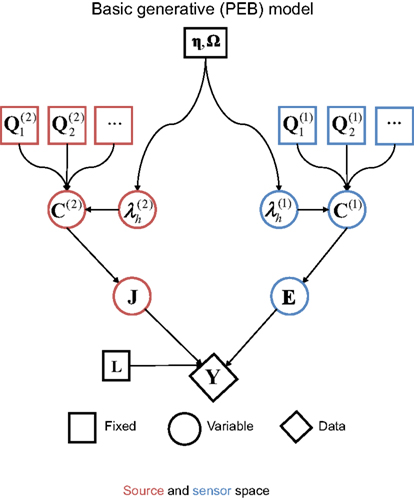
Figure 1. A Bayesian dependency graph representing the basic generative model used for the EEG/MEG inverse problem for one subject and one sensor-type (modality) within the Parametric Empirical Bayesian (PEB) framework. The variables are defined in Eqs 2–4 in the text.

Note that the assumption of a zero-mean for the sources in the second term in Eq. 3 means that C⁽²⁾ functions as a “shrinkage prior” on the sources. Indeed, it can be shown that when the source covariance matrix is the identity matrix (i.e., Q⁽²⁾ = I_p ⇒ C⁽²⁾ = exp(λ⁽²⁾)I_p, where I_p is a p × p identity matrix), the posterior (conditional) mean of J (see below) corresponds to the standard “L2 minimum norm” (MMN), or Tikhonov, solution (Mosher et al., 2003; Hauk, 2004; Phillips et al., 2005). The MMN solution explains data with minimal source energy, where the relative weighting of data fit and source energy is controlled by a regularization parameter, whose value is often derived from an empirical estimate of the signal-to-noise ratio (Fuchs et al., 1998). An elegant aspect of the above Empirical Bayesian formulation is that the degree of regularization is controlled by the hyperparameters, , whose values are optimized in a principled manner based on maximizing (a bound on) the model evidence (see below, and Phillips et al., 2005).

Furthermore, the general formulation above allows multiple spatial priors, on both the sources and the sensors. At the sensor-level, for example, one could assume separate white-noise components for each type of sensor (see Application 1 below), and/or further empirical estimates of (non-brain) noise sources; e.g., from empty-room MEG recordings (Henson et al., 2009a). At the source level, one could add additional smoothness priors (Sato et al., 2004; Friston et al., 2008), or in a more extreme case, one could use hundreds of cortical “patches” within the solution space, to encourage a sparse solution. The latter “multiple sparse priors” (MSP) approach (Friston et al., 2008) entails , where q_h ∈ ℝ^{p × 1} are sampled from a p × p matrix that encodes the proximity of sources within the cortical mesh.

With many hyperparameters (and a potentially complex cost function for gradient ascent; see below), it becomes prudent to further constrain their values, using normal hyperpriors:

where λ is a vector of hyperparameters concatenated over source and sensor levels. A (weak) shrinkage hyperprior can be implemented by setting η = −4 (i.e., a small prior mean of exp(−4) for each covariance component; though strictly speaking, the log-covariance has prior mean of −4) and Ω = 16 × I (i.e., a large prior variance, allowing to vary over several order of magnitude; Henson et al., 2007). This furnishes a sparse distribution of hyperparameters, where those that are not helpful (in maximizing the model evidence) shrink to zero; such that their associated covariance components are effectively switched off. This is a form of automatic model selection (Friston et al., 2007), in that the optimal model will comprise only those covariance components with non-negligible hyperparameters².

Model Inversion

The optimal (conditional) mean and covariance of the hyperparameters () are found using a Variation Bayesian approach under the Laplace approximation (Friston et al., 2007). This maximizes a cost function called the variational “free-energy,” under the Laplace assumption:

The free-energy is related to the log of the model evidence; i.e., given a generative model M defined by Eqs 2–4, then:

If the generative model were linear in the (hyper) parameters, this approximate equality would be exact. However, in our case, the model is effectively a Gaussian process model and is therefore non-linear in the hyperparameters. This renders the free-energy a lower bound on log-evidence, but one that has been shown to be effective in selecting between models of the present type (Friston et al., 2007). For the generative model in Figure 1, the free-energy is (ignoring constants):

where C = LC⁽²⁾L^T + C⁽¹⁾, C^(l) = Σ_h exp , and η,Ω are the means and variances respectively of the (hyper)prior distributions of hyperparameters, as in Eq. 4 (see Friston, et al., 2007, for details). The free-energy can also be considered as the difference between the model accuracy (ℱ_a, the first two terms) and the model complexity (ℱ_c, the second two terms). Heuristically, the first two terms represent the probability of the data under the assumption they have a covariance C. This follows directly from Gaussian assumptions about random effects in the model. The second two terms represent the departure or divergence of the hyperparameters (encoding the covariance) from our prior beliefs. This reports the complexity of the model (i.e., the effective number of parameters that are used to explain the data).

Having estimated the hyperparameters, the posterior estimate (conditional mean) of the sources is given by:

where P is the inverse operator, which is evaluated at the conditional means of the hyperparameters . For more precise description of the algorithm and update rules (in the general case considered in Applications 1–3 below), see Figure 2.

FIGURE 2

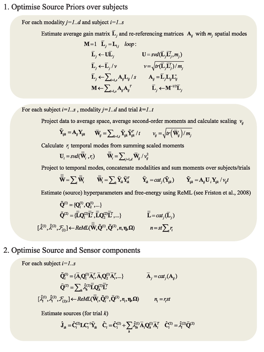
Figure 2. Full pseudocode description for multi-subject, multi-modal MNM inversion based on spm_eeg_invert. m in SPM8. For details of the ReML algorithm and its precise updates using a Fisher-Scoring ascent on free-energy cost function, see Friston et al. (2008). (Note that an alternative “greedy search” algorithm is used for maximizing the free-energy in the case of MSP inversions.) The two main stages are: (1) optimizing the source component hyperparameters over subjects (by re-referencing each subject’s gain matrix and data to an “average” space), and (2) optimizing the sensor and source hyperparameters separately for each subject, using the single optimized source component from stage 1. For a single subject, the first stage has negligible effect. Note also that this example assumes a single set of k trials: the full code allows for different numbers of trials for different numbers of conditions. We have also ignored any filtering or temporal whitening of the data (see Friston et al., 2006, for more details). ⁺ refers to the pseudoinverse; cat_j refers to the vertical concatenation of a vector or matrix along the j-th dimension; tr refers to the trace of a matrix; X = svd(Y, m) refers to a single-value decomposition of the matrix Y in order to produce the matrix X containing the m singular vectors with the highest singular values. Note that these update rules are generic – i.e., apply to all Applications in this paper – all that changed across Applications was the choice of data (Y) and covariance components (Q), as illustrated in the generative models shown in subsequent Figures.

Note that the free-energy (Eq. 5) is only a function of the mean and covariance of the hyperparameters (empirical prior source covariances) and not the parameters (source solution), which are essentially eliminated from the free-energy cost function. This is crucial because it means the real inverse problem lies in optimizing the empirical priors on the sources, not the sources per se; the source solution is a rather trivial problem that is solved with Eq. 6, once the hard problem has been solved. Classical inverse solutions (e.g., MMN and beamforming) use Eq. 6 and ignore the hard problem by making strong assumptions about the prior covariance (i.e., by assuming full priors). By using a hierarchical model, these priors become empirical and can be optimized under parametric (Gaussian) assumptions. This allows us to extend the optimization of spatial priors to include multiple modalities and subjects; something that classical solutions cannot address (optimally). Before extending this PEB framework to multi-modal and multi-subject integration, we introduce the example dataset used to illustrate this integration.

Methods and Procedure

Subjects and Experimental Design

Eighteen healthy young adults (eight female) were drawn from the MRC Cognition and Brain Sciences unit Volunteer Panel. The study protocol was approved by the local ethics review board (CPREC reference 2005.08). The paradigm was similar to that used previously under EEG, MEG, and fMRI (Henson, et al., 2003; Henson et al., 2009a). A central fixation cross (presented for a random duration of 400–600 ms) was followed by a face or scrambled face (presented for a random duration of 800–1000 ms), followed by a central circle for 1700 ms. The faces/scrambled faces subtended horizontal and vertical visual angles of approximately 3.66° and 5.38°. As soon as they saw the face or scrambled face, subjects used either their left or right index finger to report whether they thought it was symmetrical or asymmetrical about a vertical axis through its center (having been instructed that this judgment corresponded to more or less symmetrical “than average,” where an idea of average symmetry was obtained from exposure to practice stimuli). This task was chosen because it can be performed equally well for faces and scrambled faces.

There were 300 different faces and 150 different scrambled faces. Of the faces, 150 were from famous people and 150 were from unfamiliar (previously unseen) people. Scrambled faces were created by a 2D Fourier transform of 150 of the face images, from which the phases were permuted before transforming back to the image space, and masking by the outline of the original face image. Scrambled faces were therefore approximately matched for spatial frequency power density and for size. Each face or scrambled face was either repeated immediately or after a lag of 5–15 intervening items. Trials with famous faces that were not recognized during a subsequent debriefing (approximately 39 on average) were ignored as invalid trials, as were trials involving unfamiliar faces incorrectly labeled as famous during debriefing (approximately 25 on average). There were thus nine types of valid trial in total (initial presentation, immediate repetition, and delayed repetition of each of famous faces, unfamiliar faces and scrambled faces), but for present purposes, no distinction was made between initial and repeated presentations, or between famous and unfamiliar faces, resulting in just two conditions of interest: all valid face trials and all scrambled face trials. Each subject performed the experiment twice (several days apart); once for concurrent MEG + EEG and once for fMRI + MRI.

On the MEG + EEG visit, 900 trials were presented in a pseudorandom order (constrained only by the two types of repetition lag), split equally across six sessions of ∼7.5 min. The mean reaction times were 894 ms for faces and 912 ms for scrambled faces. For the fMRI + MRI session, the 900 trials were divided into nine sessions of 7 min, and within each session, blocks of ∼18 trials were separated by 20 s of passive fixation (in order to estimate baseline levels of activity).

MEG + EEG Acquisition

The MEG data were recorded with a VectorView system (Elekta Neuromag, Helsinki, Finland), with a magnetometer and two orthogonal planar gradiometers located at 102 positions within a hemispherical array in a light Elekta-Neuromag magnetically shielded room. The position of the head relative to the sensor array was monitored continuously by feeding sinusoidal currents (293–321 Hz) into four head-position indicator (HPI) coils attached to the scalp. The simultaneous EEG was recorded from 70 Ag–AgCl electrodes in an elastic cap (EASYCAP GmbH, Herrsching-Breitbrunn, Germany) according to the extended 10–10% system and using a nose electrode as the recording reference. Vertical and horizontal EOG (and ECG) were also recorded. All data were sampled at 1.1 kHz with a low-pass filter of 350 Hz. Subjects were seated, and viewed the stimuli that were projected onto a screen ∼1.33 m from them.

A 3D digitizer (Fastrak Polhemus Inc., Colchester, VA, USA) was used to record the locations of the EEG electrodes, the HPI coils and approximately 50–100 “head points” along the scalp, relative to three anatomical fiducials (the nasion and left and right pre-auricular points).

fMRI + MRI Acquisition

MRI data were acquired on a 3T Trio (Siemens, Erlangen, Germany). Subjects viewed the stimuli via a mirror and back-projected screen. A T1-weighted structural volume was acquired with GRAPPA 3D MPRAGE sequence (TR = 2250 ms; TE = 2.99 ms; flip-angle = 9°; acceleration factor = 2) with 1 mm isotropic voxels. Two FLASH sequences, and a DWI sequence, were also acquired, but are not utilized here. The fMRI volumes comprised 33 T2-weighted transverse echoplanar images (EPI; 64 mm × 64 mm, 3 mm × 3 mm pixels, TE = 30 ms) per volume, with blood oxygenation level dependent (BOLD) contrast. EPIs comprised 3 mm thick axial slices taken every 3.75 mm, acquired sequentially in a descending direction. A total of 210 volumes were collected continuously with a repetition time (TR) of 2000 ms. The first five volumes discarded to allow for equilibration effects.

These data will be available for download from http://central.xnat.org as part of the BioMag2010 data competition (Wakeman and Henson, 2010).

MEG + EEG Pre-Processing

External noise was removed from the MEG data using the temporal extension of signal-space separation (SSS; Taulu et al., 2005) as implemented with the MaxFilter software Version 2.0 (Elekta-Neuromag), using a moving window of 4 s and correlation coefficient of 0.98 (resulting in removal of 0–9 components, with an average of six across participants/windows). The MEG data were also compensated for movement every 200 ms within each session. The total translation between first and last sessions ranged from 0.74–9.39 mm across subjects (median = 3.34 mm).

Manual inspection identified a small number of bad channels: numbers ranged across subjects from 0–12 (median of 1) in the case of MEG, and 0–7 (median of 1) in the case of EEG. These were recreated by MaxFilter in the case of MEG, but rejected in the case of EEG. After reading data from all three sensor-types into a single SPM8 data format file³, the data were epoched from −500 to +1000 ms relative to stimulus onset (adjusting for the 34-ms projector delay), adjusted for the mean across the −500 to 0-ms baseline, and down-sampled to 250 Hz (using an anti-aliasing low-pass filter of approximately 100 Hz). Epochs in which the EOG exceeded 150 μV were rejected (number of rejected epochs ranged from 0 to 311 across subjects, median = 76), leaving approximately 400 valid face trials and 245 valid scrambled trials on average. The EEG data were re-referenced to the average over non-bad channels.

It is these epoched, pre-processed datasets that were used in the three PEB applications below. For simplicity, only the magnetometer data are reported here; i.e., “MEG” refers to the 102 magnetometer channels (results from planar gradiometers can be obtained from the authors; see also Henson et al., 2009a).

In order to determine a time–frequency window on which to focus for the source analysis (i.e., to select data features of interest), a time–frequency analysis was performed over the sensors using fifth-order Morlet wavelets from 6 to 90 Hz, centered every 2 Hz and 20 ms. The logarithm of the resulting power estimates was baseline-corrected (by subtracting the mean log-transformed power at each frequency during the −500 to 0-ms period). The 2D time–frequency data were then averaged over trials and channels (of a given modality) and analyzed with statistical parametric mapping (SPM). We used a paired t-test of the mean difference between faces and scrambled faces across subjects, with the resulting statistical map corrected for multiple comparisons across peristimulus times and frequencies using Random Field Theory (Kilner and Friston, 2010).

Using an initial peak threshold of p < 0.001 (uncorrected), only one cluster showed greater source energy for faces than scrambled faces that survived correction for its extent within the time–frequency space in the EEG data, which ranged between 8 and 18 Hz and from 100 to 220 ms (Figure 3A). A similar cluster was found in the MEG data, but did not quite survive correction for extent. No reliable increases in power were found for scrambled faces relative to faces. This face-related power increase coincided with a general increase in power for faces and scrambled faces relative to pre-stimulus baseline, which was distributed maximally over posterior EEG sensors and lateral MEG sensors (Figure 3B), and coincided with an evoked component that peaked around 160 ms (corresponding to the N170 and M170 for EEG and MEG components respectively, Henson et al., 2010).

FIGURE 3

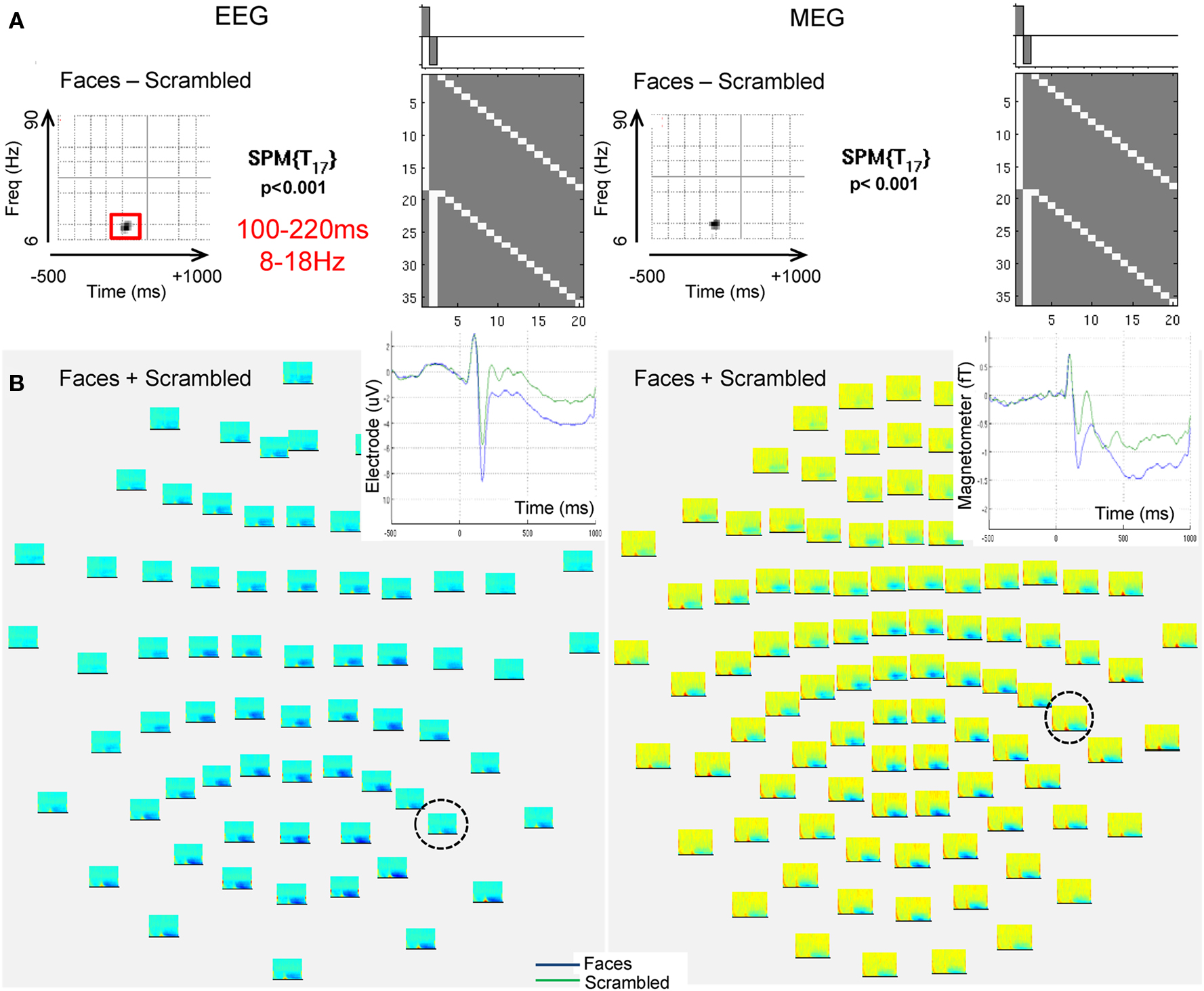
Figure 3. The EEG and MEG data used to illustrate applications of PEB. (A) Shows a thresholded, 2D Statistical Parametric Map (SPM) for a mass univariate paired t-test across the 18 subjects (corresponding to the GLM inset) testing for increases in the (log of the) total energy (induced and evoked) for faces relative to scrambled faces every 2 Hz between 6 and 90 Hz (y-axis of SPM) and every 20 ms between −500 and +1000 ms (x-axis is SPM) based on a Morlet Wavelet decomposition of data from each sensor, followed by averaging over these sensors. The peak threshold corresponds to p < 0.001 uncorrected, with the extent of the time–frequency region outlined in red for EEG surviving p < 0.05 (corrected) for multiple comparisons, using Random Field Theory (a similar region can be seen in the MEG data). (B) Shows time–frequency plots of total log-energy separately for each sensor for the average response to faces and scrambled faces. Inset is the trial-averaged evoked response for the sensors [circled in (B)] that showed maximal energy increases versus baseline, with the blue line corresponding to faces and the green line corresponding to scrambled faces (i.e., showing the evoked N/M170 component that is likely to be the dominant component of the energy increase between 8 and 18 Hz, 100 and 220 ms, for faces relative to scrambled faces).

MRI + fMRI Pre-Processing

Analysis of all MRI data was performed with SPM8. The T1-weighted MRI data were segmented and spatially normalized to gray matter, white matter, and CSF segments of an MNI template brain in Talairach space (Ashburner and Friston, 2005).

After coregistering the T2* -weighted fMRI volumes in space, and aligning their slices in time, the volumes were normalized using the parameters from the above T1 normalization, resampled to 3 mm × 3 mm × 3 mm voxels, and smoothed with an isotropic 8 mm full-width-at-half-maximum (FWHM) Gaussian kernel. The time-series in each voxel were scaled to a grand mean of 100, averaged over all voxels and volumes.

Statistical analysis was performed using the usual summary statistic approach to mixed effects modeling. In the first stage, neural activity was modeled by a delta function at stimulus onset and the ensuing BOLD response was modeled by convolving these with a canonical hemodynamic response function (HRF) to form regressors in a general linear model (GLM). Voxel-wise parameter estimates for the resulting regressors were obtained by maximum-likelihood estimation, treating low-frequency drifts (cut-off 128 s) as confounds, and modeling any remaining (short-term) temporal autocorrelation as an autoregressive AR(1) process.

Images of the parameter estimates for each voxel comprised the summary statistics for the second-stage analysis, which treated subjects as a random effect. Contrast images of the canonical HRF parameter estimates for each subject were entered into a repeated-measures ANOVA, with the nine conditions (correcting for non-sphericity of the error, Friston et al., 2002). An SPM of the F-statistic was then computed to compare the average of the (six) face conditions against that of the (three) scrambled conditions. This SPM{F} was thresholded for regions of at least 10 contiguous voxels that survived the peak threshold of p < 0.05 (family-wise error-corrected across the whole-brain). This analysis produced three clusters, in right mid-fusiform, right lateral occipital cortex, and a homologous cluster on the left that encompassed both fusiform and occipital regions. All these regions evidenced a higher BOLD signal for faces than scrambled faces (reported later in Figure 6B). These clusters are in general agreement with previous fMRI studies reporting a similar contrast of faces versus non-face objects (e.g., a subset of Henson et al., 2003), most likely corresponding to what have been called the “FFA” and “OFA” (Kanwisher et al., 1997). After a nearest-neighbor projection to the vertices in the template cortical mesh (which has a one-to-one correspondence with vertices in each subject’s canonical mesh; see below), the F-values in each cluster were binarized to form three prior spatial (diagonal) covariance components with 18, 38, and 33 non-zero entries (see Results below).

EEG/MEG Forward Modeling

The inverse of the spatial normalization used to map each subject’s T1-weighted MRI image to the MNI template was used to warp a cortical mesh from that template brain back to each subject’s MRI space (see Mattout et al., 2007 for further details). The resulting “canonical” mesh was a continuous triangular tessellation of the gray/white matter interface of the neocortex (excluding cerebellum) created from a canonical T1-weighted MPRAGE image in MNI space using FreeSurfer (Fischl et al., 2001). The surface was inflated to a sphere and down-sampled using octahedra to achieve a mesh of 8196 vertices (4098 per hemisphere) with a mean inter-vertex spacing of ∼5 mm. The normal to the surface at each vertex was calculated from an estimate of the local curvature of the surrounding triangles (Dale and Sereno, 1993). The same inverse-normalization procedure was applied to template inner skull, outer skull and scalp meshes of 2562 vertices.

The MEG and EEG sensor positions were projected onto each subject’s MRI space by a rigid-body coregistration based on minimizing the sum of squared differences between the digitized fiducials and the manually defined fiducials on the subject’s MRI, and between the digitized head points and the canonical scalp mesh (excluding head points below the nasion, given absence of the nose on the T1-weighted MRI). The gain matrix (L) was then created within SPM8 by calls to FieldTrip functions⁴, using a single shell based on the inner skull mesh for the MEG data (Nolte, 2003), and a three-shell boundary element model (BEM) based on inner skull, outer skull and scalp meshes for the EEG data (Fuchs et al., 2002). Lead fields for each sensor were calculated for a dipole at each point in the canonical cortical mesh, oriented normal to that mesh.

EEG/MEG Inversion Parameters

A spatial dimension reduction was achieved by singular-value decomposition (SVD) of the outer product of the gain matrix, with a cut-off of exp(−16) for the normalized eigenvalues (which retained over 99.9% of the variance). This produced m = 55 − 68 spatial modes across subjects for the MEG (magnetometer) data, and m = 61 − 69 for the EEG data (see Figure 2).

Based on the suprathreshold SPM results for comparison of faces versus scrambled faces in the sensor time–frequency analysis (see above), the data were projected onto a (Hanned) time window between +100 and +220 ms, and a frequency band from 8 to 18 Hz. The resulting covariance across sensors was averaged across all trials of both trial-types (faces and scrambled), effectively capturing induced and evoked power (Friston et al., 2006). A temporal dimension reduction was achieved by an SVD of this mean covariance, once projected onto the spatial modes, using a cut-off of exp(−8) for the normalized eigenvalues (which retained over 95% of the variance; see Figure 2). This resulted in r = 3 temporal modes for every subject (Friston et al., 2006). Thus the covariance matrices for each modality of approximately 63 × 63 (reduced sensors × sensors) on average were estimated from approximately 645 × 3 (trials × reduced time points) samples.

For simplicity (and to highlight to benefits of fMRI priors), we used simple generative models with a single source component (the identity matrix, , i.e., MMN model) for source reconstruction (Table 1). Having estimated the inverse operator, P (Eq. 6), the power of the source estimate for each condition (within the same time–frequency window, averaged across trials) was calculated for each vertex, and smoothed across vertices using eight iterations of a graph Laplacian. The logarithm of these smoothed power values was then truncated (to remove very small values), scaled by the resulting mean value over vertices and trials, and interpolated into a 3D space of 2 mm × 2 mm × 2 mm voxels. Finally, the 3D images were smoothed with an isotropic 3D Gaussian with a FWHM of 8 mm (to allow for residual inter-subject differences). Note that the inverse operator is estimated from the covariance across sensors over a range of times/frequencies within the time–frequency window of interest (more precisely, by the temporal modes resulting after SVD of the data filtered to this window, as above), which can be used to reconstruct a timecourse for each source; it is only when subsequently performing statistics on power estimates that such source estimates are averaged across time and frequency to produce a single scalar value for each source.

TABLE 1

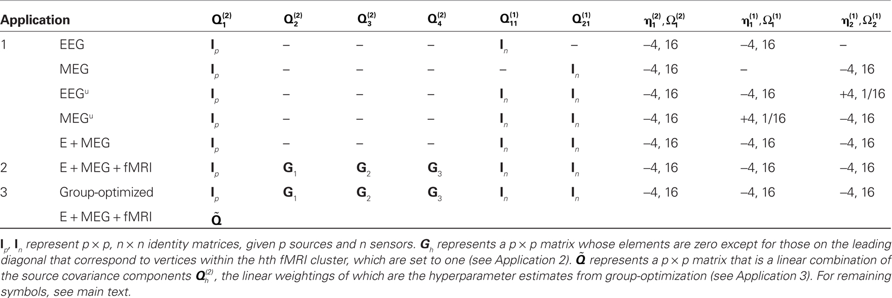
Table 1. Summary of the differences in generative model across Applications 1–3.

Results

In this section we present the results of model inversion using the exemplar data of the previous section. We focus on three generalizations of the basic model above that enable (symmetric and asymmetric) fusion of different imaging modalities and, finally, the fusion of data from different subjects. Note that the same optimization scheme was used for all three Applications (as shown in Figure 2); the only difference across Applications was the specific choice of covariance components at source and/or sensor levels, (as shown in Table 1).

Application 1: Fusion of EEG and MEG Data

The first extension of the basic generative model (Figure 1) is to a symmetric fusion model of MEG and EEG data (Henson et al., 2009a). This is shown schematically in Figure 4. Effectively, this corresponds to concatenating the data, gain matrices, and sensor error terms for each sensor-type, such that Eq. 1 becomes, for j = 1…d sensor-types:

FIGURE 4

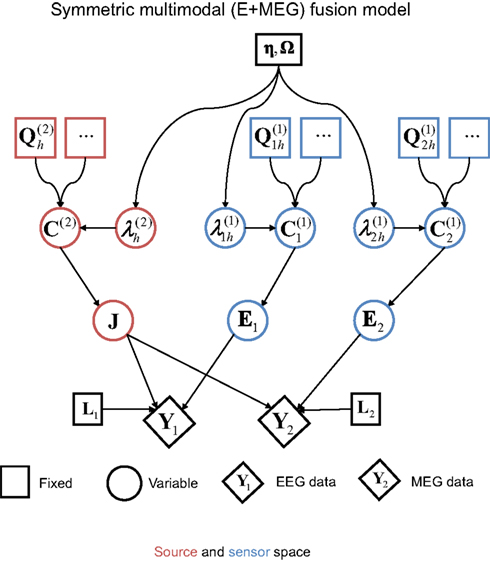
Figure 4. The extension of the generative model in Figure 1 to the fusion of EEG and MEG data, i. e., j = 1–2modalities (Y₁ and Y₂). This model was the one used to produce the results in Figure 5; i.e., with one minimum norm source prior (, where I_p is a p × p identity matrix for the p sources) and one white-noise sensor component for each modality (, where n_j is the number of sensors for the j-th sensor-type).

To accommodate different scaling and measurement units across the different sensor-types, the data and gain matrices are re-scaled (after projection to the m_j spatial modes) as follows:

where tr(X) is the trace of X. This effectively normalizes the data so that the average second-order moment (i.e., sample variance if the data are mean-corrected) of each spatial mode is the average variance expected under independent and identical sources with unit variance (ignoring sensor noise). If the gain matrices for each sensor-type were perfect (and expressed in the same physical units), this scaling would be redundant. In the absence of such knowledge however, it allows for arbitrary scaling of the lead fields from different modalities and enables the relative levels of sensor noise to be estimated for each sensor-type; those levels being proportional to . This is arguably more principled than estimating relative noise levels from, for example, the pre-stimulus period (e.g., Molins et al., 2007), which does not discount brain “noise” from the sources⁵. For tests of the validity of this scaling, and further discussion, see Henson et al. (2009a).

Note that the sources in J and their priors (left-hand branch of Figure 4) are unchanged. It is the sensor-level covariance components (right-hand branches of Figure 4) that are augmented. Specifically, the sensor error covariance, C⁽¹⁾, becomes:

where for each sensor-type j is again estimated by a linear combination of covariance components:

For simplicity, we restrict the present example to just h = 1 sensor–noise component per sensor-type, equal to the identity matrix (i.e., isotropic or white-noise), .

Because the model evidence is conditional on the data, one cannot evaluate the advantage of fusing MEG and EEG simply by comparing the model evidence for the fused model (Figure 4) relative to that for a model of the MEG or the EEG data alone (Figure 1). Rather, one can fit the concatenated (MEG and EEG) data, and compare the model evidence for “unimodal” versus “bimodal” models by varying the sensor-level hyperpriors for each sensor-type (Eq. 4). If we increase the hyperprior mean for the j-th sensor-type to (i.e., a proportional increase in the prior noise variance of exp(8)≈3000) and decrease its hyperprior variance to (i.e., tell the model we are confident the j-th modality is largely noise), then we are effectively discounting data from that sensor-type. This is because the noise for that sensor-type is modeled as very high relative to the other modality. Because such hyperpriors are part of the model, their veracity can be compared using the free-energy approximation to the log-evidence in the usual way. In other words, if the j-th modality is uninformative, then the “unimodal” model for the other modality will have more evidence than the “bimodal model.” More specifically, we can use the free-energy (Eq. 5) to test whether a “bimodal” fusion model with symmetric and weak shrinkage hyperpriors (i.e., and for j = 1 and j = 2) has more evidence than either of the two “unimodal” models that effectively discount the other modality with an asymmetric noise hyperprior ( and for j = 1 or j = 2). See Table 1 for a summary of the different models used in this Application.

The resulting free-energies for each of these three models – unimodal EEG (MEG discounted), unimodal MEG (EEG discounted) or bimodal EEG + MEG are shown in the leftmost panel of Figure 5. In nearly all subjects (shown by lines), the bimodal (fused) model has a higher evidence than either unimodal model, as confirmed by two-tailed, paired t-tests relative to unimodal EEG: t(17) = 3.70, p < 0.005, and relative to unimodal MEG, t(17) = 2.98, p < 0.01. This advantage of fusion was manifest both in improved model accuracy (middle panel), one-tailed t > 2.71, p < 0.05, and reduced model complexity (rightmost panel), one-tailed t > 1.88, p < 0.05, relative to both unimodal models. These results complement and extend our previous evaluation of MEG + EEG fusion, where we examined the change in the posterior precision of the source estimates (Henson et al., 2009a).

FIGURE 5

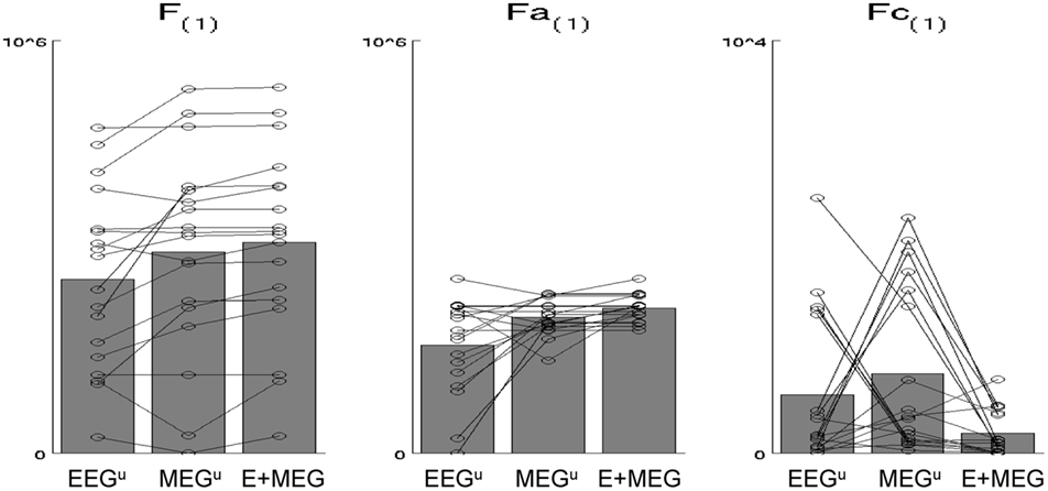
Figure 5. The bars in the leftmost plot show the mean across subjects of the maximized free-energy (F) bound on the model log-evidence (arbitrary units) for (1) “unimodal” EEG model (EEG^u), (2) “unimodal” MEG model (MEG^u), and (3) bimodal “fusion” model (E + MEG). All models explain the same concatenated EEG and MEG data (projected to the time–frequency window identified in Figure 3), but “unimodal” models have a sensor-level hyperprior with a high mean and precision for the other modality, which effectively discounts data of that modality as noise (see text). The circles joined by lines show the results for each individual subject. The middle and rightmost plots show the two parts of the free-energy: the accuracy (F_a) and the model complexity (F_c); see text for details (note that these differ by constant terms that not included here). The advantage of EEG and MEG fusion is reflected by the increase in F and F_a, and decrease in F_c.

The reconstructed sources also show differences between the separate and fused inversions (Figure 6A). The mean source power across subjects on the MNI cortical surface is similar for all three models (see maximum intensity projections – MIPs – inset in the top right of each column), with a predominance of power in bilateral occipito-temporal cortex, especially on the right. The reliability of this pattern across subjects, as reflected by t-values surviving p < 0.001 uncorrected within the MNI volumetric space (the main MIPs in each column), were more different across inversions however, being greater on the left in the case of EEG alone and greater on the right in the case of MEG alone. Importantly however, the t-values for the bimodal model recovered a bilateral pattern, which also spread more anteriorly along the ventral surface of the temporal lobe (consistent with the fMRI data in Figure 6B). Indeed, the maxima in left (−30 −60 −14) and right (+42 −72 −14) fusiform survived correction for multiple comparisons across the volume, t(17) > 6.40, p < 0.05 corrected. This more plausible source reconstruction following fusion of EEG and MEG echoes that found when using MSP in Henson et al. (2009a).

FIGURE 6

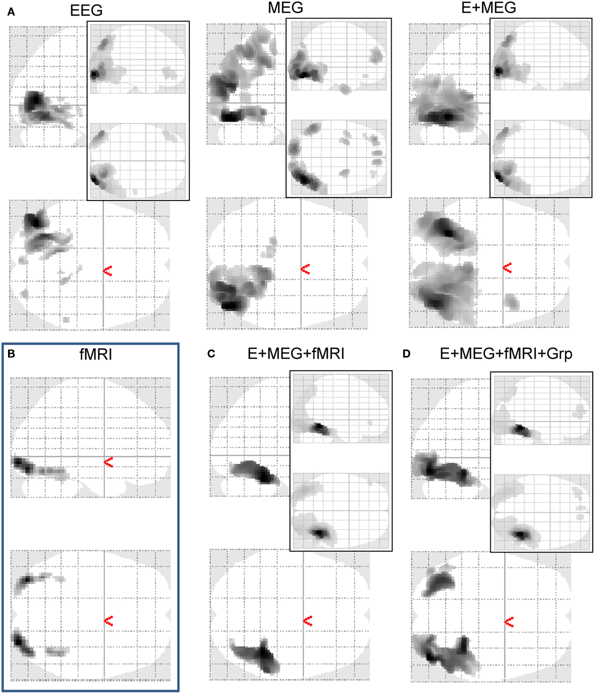
Figure 6. Maximal Intensity Projections (MIPs) in MNI space for increases in the log-energy for faces, relative to scrambled faces, within a 100 to 220-ms, 8–18 Hz time–frequency window. The MIPs inset to the top right of each panel show the average increase in this face-related energy across subjects for the 512 vertices showing the maximal such increase. The main MIPs in each panel represent SPMs of the corresponding t-statistic (thresholded at p < 0.001 uncorrected), after interpolating the cortical source energies for each subject into a 3D volume. (A) shows (from left to right) the results for inverting EEG data alone, MEG data alone, or from fusing EEG and MEG data in the “bimodal” model of Figures 4–5. (B) shows the results of the same contrast but on the fMRI data (though two-tailed, and at a higher threshold of p < 0.05 corrected for multiple comparisons). (C) shows the results of inverting EEG and MEG data after the addition of three fMRI priors [those in (B)] using the generative model shown in Figure 7. (D) Shows the results of group-optimization of the fMRI priors used in (C), using the generative model shown in Figure 10.

Application 2: Asymmetrical Integration of EEG and MEG Data with fMRI Data

The second extension of the basic generative model is to an integration of MEG and EEG with fMRI (Henson et al., 2010), as shown in Figure 7. This corresponds to asymmetric multi-modal integration (as distinct from the symmetric integration in the previous section; Daunizeau et al., 2005), in the sense that the fMRI data are not fit simultaneously with the MEG and EEG data (i.e., do not appear at the bottom of the dependency graph in Figure 7), but rather are used to define the prior covariance components on the sources (i.e., the fMRI data correspond to the third data type, Y₀, at the top of the graph). The reason for this is reviewed later.

FIGURE 7

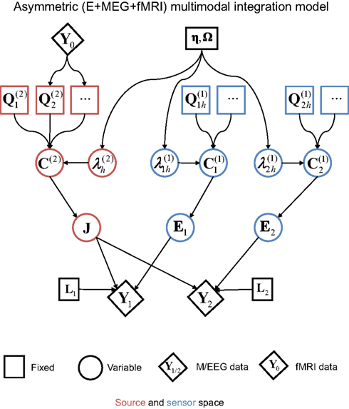
Figure 7. The extension of the generative model in Figure 4 to the addition of fMRI priors (Y₀).

To map fMRI data to a (small) number of covariance components ( in Figure 7), the typical procedure is to threshold an SPM of the relevant contrast of fMRI data to produce a number of clusters (contiguous suprathreshold voxels). These clusters can then be projected to the nearest corresponding vertices in each subject’s cortical mesh. Here the canonical cortical mesh (Mattout et al., 2007) is useful, because this provides a one-to-one mapping between the vertices of each subject’s cortical mesh and the vertices in standard (e.g., MNI) space. This allows the fMRI clusters to be defined by different subjects, or, as here, by group statistics on spatially normalized fMRI data across subjects. Figure 6B shows a MIP of clusters of at least 10 voxels, whose peak statistical values survived p < 0.05 (corrected) for multiple comparisons across the brain, where that statistic is the F-value for a two-tailed⁶ paired t-test of faces versus scrambled faces across the same 18 subjects whose EEG/MEG data are considered here. This furnished three clusters, in right fusiform and right lateral occipital cortex, plus a single cluster encompassing similar regions on the left. Each cluster gives a vector, q_h, across vertices for the h-th cluster, whose values are the interpolated fMRI activation values for each vertex within that cluster, and zero otherwise. The corresponding source prior covariance component is then:

where G(·) is some matrix function, and f(x) is some scalar “linkage” function (linking fMRI activation values, which could be statistic values or % signal change, to EEG/MEG prior covariance terms). Here, we use a Heaviside linkage function corresponding to f(x) = 1 for x > 0, and f(x) = 0 otherwise, and G(·) = diag(·) (which puts the values of f on the leading diagonal of a matrix), since such simple “binary, variance” priors were sufficient for similar data in Henson et al. (2010). In other words, the prior variance for all vertices within a cluster was equal (regardless of the F-value of the corresponding voxels in the fMRI analysis), and the prior covariance between vertices was zero [positive covariance could be introduced by setting G(·) to the identity function; i.e., defining covariance components by the outer product of f(q_h)].

An important aspect of this approach to integration of fMRI with EEG/MEG is that each fMRI cluster contributes a distinct covariance component; i.e., each cluster can be up- or down-weighted by its own hyperparameter, (for further discussion and evidence for this claim, see Henson et al., 2010). This allows for the fact that the neural activity giving rise to the BOLD data might not be expressed proportionally in E/MEG data. Note that this approach is fundamentally different from assuming (ad hoc) fixed values for the variance of source activity in these regions (cf, Liu et al., 1998), but is functionally similar to having a separate hyperprior for the variance (or precision) at each source location, and increasing the mean (or dispersion) of that hyperprior for locations corresponding to significant fMRI signal (Sato et al., 2004)⁷. In other words, each fMRI activation locus may, after the hyperparameters have been optimized, show a greater or smaller variance than other components not based upon fMRI. One important example of this dissociation between fMRI and electromagnetic activation would be when the fMRI data in one or more regions reflects neural activity arising before or after the time window of E/MEG data modeled (given the much slower dynamics of the BOLD signal). For example, it is possible that some of the clusters in the present fMRI data reflect neural activity that is related to face processing but outside our 100–220 ms time window (see Henson et al., 2010, for further discussion). The ability of this approach to discount such “invalid” spatial priors has previously been demonstrated by simulation (Phillips et al., 2005; Mattout et al., 2006).

For real data, the effect of adding the three fMRI source priors to the basic MMN prior (the identity matrix ) on the free-energy for each combination of sensor-type – EEG data alone, MEG data alone, or fused EEG + MEG data – is shown in Figure 8A. In nearly all subjects, the addition of the fMRI priors increased the free-energy significantly for each sensor-type, resulting in a significant improvement on average, t(17) > 3.46, p < 0.005. The impact on source reconstruction for the fused EEG + MEG case is shown in Figure 6C, where it can be seen that the fMRI priors have “pulled” the source energy to the right fusiform region, in terms of both the mean source energy on the surface (inset) and group-level statistics in volumetric space. Indeed, while there are no longer any maxima that survive whole-brain correction, the t-value of the right fusiform maximum with fMRI priors (+40 −42 −22) increased from 4.21 (without fMRI priors) to 4.68 (with fMRI priors). Note also that the mean source energy is not only more focal, relative to the model without fMRI priors (inset in rightmost panel of Figure 6A), but also more anterior, i.e., “deeper” (further from the sensors). This shows how fMRI priors can overcome the well-known bias of the MMN solution toward diffuse superficial source estimates (the reason may be due in part to the sparsity afforded by discrete, compact priors, in the same way that others have shown how sparse priors reduce the superficial bias of L2-norm based inverse solutions; Trujillo-Barreto et al., 2004; Friston et al., 2008). Note however that the “sparseness” of such fMRI priors will depend on the threshold used to define the fMRI clusters (e.g., we would obtain fewer and larger clusters had we reduced the statistical threshold)⁸.

FIGURE 8

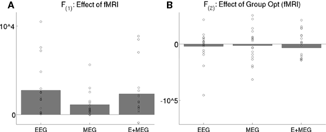
Figure 8. The bars show the difference in the mean across subjects of the maximized free-energy bound on the model log-evidence (arbitrary units) for two models: with versus without the three fMRI priors (A), or with versus without group-optimization of those priors (B), for EEG data alone, MEG data alone, or the combined EEG and MEG data. The circles show values for each subject’s difference. fMRI priors significantly improve the mean free-energy, but their group-optimization does not (as expected, see text). F₍₁₎ refers to the maximal free-energy from the first stage of group-optimization of the fMRI source hyperparameters, whereas the F₍₂₎ refers to the maximal free-energy from the second stage of individual inversion of each subject when using the group-optimized source prior (see Figure 2).

A symmetrical fMRI + E/MEG fusion model?

It is worth noting at this point that one could also consider a symmetric version of E/MEG and fMRI integration, one possible example of which shown in Figure 9 (see also Luessi et al., 2011). Here, a common set of electrical sources (J) generate both the E/MEG and fMRI data. In this case, the (spatial) forward model for the fMRI data (L₀) is relatively simple; e.g., a spatial smoothing kernel that depends on the spatial dispersion of the BOLD signal and spatial resolution (voxel-size) of the fMRI data (relative to the density of the electrical sources modeled). The separate error component for the fMRI data can also be relatively simple, e.g., a similar spatial smoothness kernel (Flandin and Penny, 2007). Note that the fMRI kernel matrix L₀ would generally have a higher ratio of rows to columns than the E/MEG gain matrix L₁; reflecting the typically greater number of fMRI measurements (voxels) than E/MEG measurements (for a single time point). In other words, the indeterminacy in the spatial mapping from electrical sources to measurements is typically much less for fMRI than E/MEG, which means that the fMRI data are likely to have the dominant effect on the estimation of the location of electrical sources. This likely dominance of the fMRI data therefore questions the value of such a symmetric fusion model. Furthermore, there are potential problems that arise when electrical sources do not produce detectable fMRI signals and vice versa.

FIGURE 9

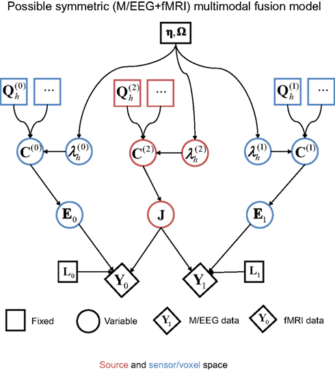
Figure 9. A possible symmetric model for fusion of EEG/MEG data and fMRI data (cf. Figure 7).

One common approach to the different spatial scales of fMRI and M/EEG is to make both the fMRI data (Y0) and M/EEG source estimates (J) depend on a third, latent variable (e.g., Trujillo-Barreto et al., 2001; Daunizeau et al., 2007; Ou et al., 2010). This variable can have a spatial prior (e.g., for smoothness, or for sparseness) that encourages a common spatial covariance structure across fMRI and M/EEG parameters (with possibly different temporal profiles). This alleviates the problems associated with having the current estimates J generate both the fMRI data and the M/EEG sensor data that is depicted in Figure 9. However, the value of such models is still unclear when one considers the vastly different temporal resolutions of the two modalities. fMRI data are typically only sampled every few seconds, and are themselves the product of a temporal smoothing of electrical activity by the HRF. Therefore a full spatiotemporal multi-modal fusion model would entail a forward model for the fMRI data that took into account hemodynamic smoothing. This could even take the form of a biophysical model with many parameters, based on physiological knowledge of hemodynamics (e.g., Sotero and Trujillo-Barreto, 2008). In this situation, there would be (temporal) information about the sources in the E/MEG data that is not present in the fMRI data. For this additional temporal information in the E/MEG data to aid estimation of the spatial distribution of the sources, or for that matter, for the ability of the additional spatial information in the fMRI data to aid estimation of the temporal profile of the sources, there would need to be some dependency between the spatial and temporal parameters controlling the electrical currents in the brain. Unfortunately, there is no principled reason to think that there will be strong dependencies of this sort, because there is no evidence that the potential range of dynamics of electromagnetic sources varies systematically across different parts of the brain. If the spatial and temporal parameters of forward models are indeed (largely) conditionally independent, then the most powerful approach to EEG/MEG and fMRI integration may be asymmetric: i.e., using EEG/MEG data as temporal constraints in whole-brain fMRI models, or using fMRI data as spatial priors on the EEG/MEG inverse problem, as considered here.

Application 3: Group-Optimization of Source Priors

The final extension of the basic generative model in Figure 1 is to the group-optimization of source priors, as shown in Figure 10. For each modality, there are now there are multiple datasets (Y_i for the i-th subject), each explained by separate source distributions (J_i) with separate error terms (E_i), but sharing the same priors. The estimation of the hyperparameters is therefore optimized by pooling data across subjects, as was originally demonstrated using several hundred sparse priors (MSP, Litvak and Friston, 2008). Here, we apply this optimization to the four source priors in the previous section, comprising the MMN constraint plus the three fMRI priors. Starting with the simple case of one modality, the basic idea for group models is to concatenate the data from i = 1…s subjects over samples:

FIGURE 10

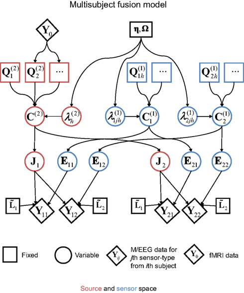
Figure 10. The extension of the generative model in Figure 7 to group-optimization of source priors, for i = 1–2 subjects, each with data from j = 1–2 modalities.

This contrasts with the model in Eq. 7 where we concatenated over channels. In multi-modal integration, we consider each new modality as an additional set of sensors that are picking up signals generated by the same sources. For multi-subject integration, the sources may be different but are deployed under the same spatial priors; because we examine subjects under the assumption that (a priori) they have the same functional anatomy. This means each subject’s data constitute a separate realization and should be treated as a further sample of the same thing. We therefore concatenate over samples (analogous to concatenating over multiple trials from one subject; Friston et al., 2006). However, to do this we must realign the subjects’ data so that the effective lead fields are the same over subjects. This is achieved by a “re-referencing” matrix, A_i, that projects each subject’s gain matrix to a common or “average” gain matrix; i.e., A_iL_i = 〈A_iL_i〉 (see also Valdés-Hernández et al., 2009, for a related approach). This average is computed with the constraint that its preserves the information (on average) in the sensor data:

This is a complicated non-linear problem that can be solved using recursive least squares and an implicit generalized eigenvalue solution (see Figure 2). Clearly, the average lead field cannot necessarily “see” all the data sampled by the original (subject-specific) lead fields. Typically about 10% of the data is lost, in the sense it lies in the null space of the average lead field. Nonetheless, this form of re-referencing is an improvement on that described in Litvak and Friston (2008), where all the lead fields were re-referenced to the first A_iL_i = L₁, under the assumption that this was representative of the remaining lead fields. The solution above is an improvement in the sense that one does not have to assume the first subject’s lead field is “representative,” and the re-referencing does not depend on which subject is designated as the “first.”

Crucially, although the sources J_i are subject-specific, the empirical source priors are the same. This prior is used in the hope that pooling data across individuals will provide extra constraints on the hyperparameters (assuming sources are sampled from a spatial prior that is common to subjects). If this prior assumption is correct, the ensuing subject-specific reconstructions should improve the consistency of the source localization across subjects (but not bias any trial-specific differences at any given location).

In practice, group-optimization entails two stages of hyperparameter optimization (see Figure 2): In the first stage, the source hyperparameters are estimated based using Eq. 9. In the secondstage, a single weighted combination of the source priors (weighted by the hyperparameters estimated in the first stage; Σ_h exp ) is combined with the sensor covariance components, and their hyperparameters estimated separately for each subject’s (unreferenced) data and gain matrix, as in Eq. 7.

We can combine multi-modal models (Eq. 7) and multi-subject models (Eq. 9), as shown in Figure 10, in order to invert joint models of the form (for d modalities and s subjects)

This is the most general form of the model currently supported by the Matlab routine spm_eeg_invert.m in SPM8.

The effect of group-inversion of the four empirical source priors on the free-energy for each combination of sensor-type is shown in Figure 8B. Group-optimization had no significant effect on the mean free-energy across subjects. This is expected: constraining the weighting of source priors across subjects gives less scope for maximizing the model evidence for any single subject (relative to a model optimized for that subject’s data alone). Indeed, in a previous application to hundreds of sparse priors, Litvak and Friston (2008) found a decrease in the mean free-energy after group-inversion. Rather, the effects of group-optimization are apparent in the statistical tests of the source estimates across subjects, as is apparent in Figure 6D. Though the mean source estimates appear little affected (inset in Figure 6D), there are many more voxels with t-values that survive thresholding (compared to Figure 6C), including a suprathreshold cluster in the left, as well as right, fusiform. In fact, group-optimization tripled the number of suprathreshold voxels (from 1,104 to 3,162) and increased the maximal t-value (in right fusiform) from 4.67 to 5.91.

The effect of group-optimization on the hyperparameters themselves is shown in Figure 11. The bars constitute a histogram of the hyperparameter estimates across subjects, for each of the four source priors after inverting each subject’s data separately, using Eq. 7. The solid vertical line is the single group-optimized estimate, and the dotted line is the hyperprior mean of h = −4. Group-optimization not only enforces a consistent ratio of hyperparameter estimates across subjects, but can also increase those estimates above the average without group-constraints. In the case of the lOFA/FFA prior (lower left panel), for example, the solid line (group-optimized estimate) is to the right of the central tendency of the histogram of individual estimates. Or in the case of the right OFA prior (upper right panel), its hyperparameter estimate was effectively shrunk to zero for some subjects without group-optimization, but remains close to the hyperprior mean (as ) with group-optimization. It should be remembered that this group-optimization assumes that the same set of cortical generators exists in all subjects, i.e., that subjects differ only in the overall scaling of this set (as reflected by single hyperparameter for each subject i in the final stage in Figure 2), and in their relative sensor-level noise components (as reflected by the hyperparameters in Figure 2). If one does not wish to make this assumption, then group-optimization need not be selected, and each subject inverted separately.

FIGURE 11

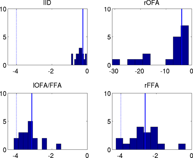
Figure 11. The hyperparameter estimates for the MMN source prior (top left) and three fMRI source priors (remaining plots; OFA, occipital face area; FFA, fusiform face area; l, left, r, right). The solid bars constitute a histogram of estimates across subjects without group-optimization; the solid line reflects the single estimate after group-optimization across subjects; and the dotted line shows their prior expectation . Note the different scale of the x-axis in the top right panel.

Discussion

We have reviewed a theoretical framework called Parametric Empirical Bayes (PEB) that we believe offers a natural and powerful way to introduce multiple constraints into the inverse problem of estimating the cortical generators of EEG/MEG data. Empirical Bayes is a general approach afforded by hierarchical formulation of linear generative models, which is explicitly or implicitly used in many other approaches to the EEG/MEG inverse problem (e.g., Baillet and Garnero, 1997; Trujillo-Barreto et al., 2001, 2008; Sato et al., 2004; Daunizeau et al., 2007; Wipf and Nagarajan, 2009; Ou et al., 2010; Luessi et al., 2011). We have illustrated three applications of PEB to an example dataset: (1) the symmetric integration (fusion) of MEG and EEG data, which entailed common source priors (a single MMN prior) but separate modality-specific sensor error components, (2) the asymmetric integration of EEG/MEG data with fMRI data, in which significant clusters in the fMRI data form additional, separate spatial priors on the EEG/MEG sources, and (3) the optimization of multiple source priors (in this case from the fMRI clusters) across subjects, by re-referencing their data and gain matrices to a common source space. The benefit of these three applications was apparent in improvements in the variational free-energy bound on the Bayesian log-evidence of the generative model, and/or improvements in the number or location of suprathreshold sources in a statistical comparison of spatially normalized source images across subjects.

One advantage of an empirical (hierarchical) Bayesian framework is that the degree of regularization of the inverse solution by prior constraints is optimized by virtue of an implicit hierarchical generative model of the data, rather than being fixed in advance. This optimization refers to the estimation of the hyperparameters in order to maximize (a bound on) the model evidence (for further elaboration, see Friston et al., 2007; Wipf and Nagarajan, 2009). So, in the case of the spatial priors from fMRI in Application 2 above, rather than assuming a fixed ratio (e.g., 10%) for the prior variance on sources with and without fMRI activations (Liu et al., 1998), the hyperparameter controlling the variance of each fMRI prior is estimated anew for each dataset⁹. Furthermore, the ability to estimate multiple hyperparameters – i.e., the influence of multiple prior constraints – is an important advance on traditional approaches to the EEG/MEG inverse problem. Application 2 described one advantage, in the context of multiple fMRI priors, when different fMRI priors can contribute differently to the EEG/MEG data. In particular, if a subset of the fMRI priors reflect neural activity that is not represented within the time/frequency window of EEG/MEG data being localized, then their hyperparameters should shrink to zero. Another example is the use of MSP (Friston et al., 2008), that furnish more focal solutions. It is the presence of multiple priors that then offers the possibility to optimize the relative value of their hyperparameters across subjects, as shown in Application 3.

A further advantage of the PEB framework is that the maximization of variational free-energy not only optimizes the hyperparameters, but its maximum also provides an upper bound on the model log-evidence. This offers a natural way to compare different generative models of EEG/MEG data. It can be used, for example, to compare different electromagnetic forward models (Henson et al., 2009b), or to optimize the number of equivalent current dipoles (Kiebel et al., 2008). Its maximization can also be used to optimize more specific details of the generative model: For example, to explore the choice of the “linkage function” that relates fMRI values (e.g., t-statistic or % signal change) to the values in the source (co)variance matrices in Application 2 above (Henson et al., 2010). One important issue for future further consideration however, particularly with many hyperparameters, is the possible existence of local maxima in the free-energy cost function (Wipf and Nagarajan, 2009).

There are clearly assumptions in this review that deserve further exploration. Some of these are specific to the above applications: For example (1) the particular type of scaling used for fusion of MEG and EEG data in Application 1 (see Henson et al., 2009a), or further adjustment of the gain matrices for multiple modalities with different sensitivities (Huang et al., 2007); (2) the possibility of symmetric fusion of E/MEG and fMRI, as discussed in Application 2; and (3) the accuracy of the re-referencing to an “average” gain matrix for multi-subject fusion in Application 3. Other assumptions are generic to the PEB framework. For example, PEB’s assumption of Multivariate Gaussian distributions is necessary to express the problem sufficiently in terms of first and second-order statistics (i.e., means and covariances). This is what makes our approach conform to the class of “L2-norm” inverse solutions (as distinct from, for example, “L1-norm” solutions, Uutela et al., 1999). This parametric approach also enables analytical tractability and reasonable computational efficiency of the matrix operations entailed. Relaxing these Gaussian assumptions (e.g., using gamma priors, Sato et al., 2004) may require more complex optimization algorithms (e.g., Wipf and Nagarajan, 2009), while relaxing the Variational assumption that the posteriors factorize may require a full Monte Carlo approach to optimization (Friston et al., 2007). Nonetheless, the underlying tenet of empirical Bayes; namely the use of hierarchical generative models, is clearly central to the development of more complex and realistic models of multi-subject and multi-modal neuroimaging data.

Software Note

All the models and inversion scheme used in this work are available in the academic software SPM8¹⁰, specifically the “spm_eeg_invert.m” routine.

Conflict of Interest Statement

The authors declare that the research was conducted in the absence of any commercial or financial relationships that could be construed as a potential conflict of interest.

Acknowledgments

This work is funded by the UK Medical Research Council (MC_US_A060_0046) and the Wellcome Trust. Correspondence should be addressed to rik.henson@mrc-cbu.cam.ac.uk. We thank Jean Daunizeau and three reviewers for helpful comments.

Footnotes

1. ^In fact, the error covariance of these distributions is assumed to factorize into temporal, V, and spatial, C, components (Friston et al., 2006), such that: vec(E^(l)) ~ 𝒩(0,V ⊗ C^(l)), where vec vectorizes a matrix and ⊗ represents the Kronecker tensor product. For simplicity, we will assume the temporal component (e.g., autocorrelations) are known, and focus here on optimizing the spatial components.
2. ^Note that, although the prior mean and variance of these hyperpriors encourage a sparse distribution of hyperparameters, such hyperpriors do not necessarily furnish a sparse distribution of parameters, i.e., a sparse distribution of source estimates.
3. ^http://www.fil.ion.ucl.ac.uk/spm
4. ^http://fieldtrip.fcdonders.nl/
5. ^For MEG data, an estimate of sensor–noise covariance can be obtained from empty-room recordings (Henson et al., 2009a), for which the noise consists of a random component intrinsic to the SQUID sensors and associated electronics, plus a component from environmental magnetic noise (that has not been fully attenuated by magnetic shielding). Methods for estimating such sensor–noise covariance for EEG data are less obvious however.
6. ^A two-tailed test was used in order to make minimal assumptions about the mapping between BOLD and EEG/MEG signals (Henson et al., 2010; though in the present data, all three clusters did show a greater BOLD signal for faces than scrambled faces). Note also that we are using fMRI priors that are defined by the difference between faces versus scrambled faces, yet inverting the E/MEG data after collapsing across both faces and scrambled faces (and only contrasting faces versus scrambled faces after estimating the sources). This is a subtle but important point that we discuss in detail elsewhere (Henson et al., 2007): In brief, this rests on the assumption that the generators of the power (within our time–frequency window) induced by faces and scrambled faces versus pre-stimulus baseline coincide with those that show differences in such power for faces versus scrambled faces. One measure of the extent to which this is a valid assumption is the free-energy: if this assumption were false, we would not anticipate an increase in free-energy when adding the fMRI priors (Henson et al., 2010).
7. ^There are important differences between the present approach and that of Sato et al. (2004): we optimize covariance components (not precisions), and use fMRI to add formal priors (in terms of components) as opposed to modulating the mean of the hyperpriors. Our approach does not suppress signal from non-fMRI areas. It would be an interesting future project to compare the two approaches formally. For present purposes, the similarity of the two approaches is more relevant, in that both provide a principled source-specific soft constraint on the reconstruction, based on fMRI.
8. ^It is interesting to consider how the effect of fMRI priors might depend on their relative “size” (spatial extent – i.e., number of non-zero elements). In general, their effect is likely to depend on the data. If the true sources overlap with only one of those components, then its hyperparameter is still likely to be greater than those of other components, even if those components have a larger spatial extent, unless there is a high correlation in the mean gain vectors associated with each cluster of vertices. In the latter case, it is possible that “bigger” components will be favored, because their hyperparameter estimate can remain smaller (less far from its shrinkage hyperprior mean) while still fitting the data as well. The same is likely to apply to covariance components with comparable spatial extent, but higher magnitudes of non-zero elements (i.e., higher prior variances on the source parameters), as might happen for example if the covariance components were a continuous (rather than binary, as here) function of the underlying fMRI statistic or fMRI signal.
9. ^The prior mean and variance of the hyperparameters (the hyperpriors), on the other hand, are fixed. Nonetheless, they are based on principled reasons, namely to provide weak shrinkage (see, for example, Application 1), and could in principle be explored by further maximization of the variational free-energy (see Henson et al., 2007).
10. ^http://www.fil.ion.ucl.ac.uk/spm

References

Ashburner, J., and Friston, K. J. (2005). Unified segmentation. Neuroimage 26, 839–851.

Pubmed Abstract | Pubmed Full Text | CrossRef Full Text

Baillet, S., and Garnero, L. (1997). A Bayesian approach to introducing anatomo-functional priors in the EEG/MEG inverse problem. IEEE Trans. Biomed. Eng. 44, 374–385.

Pubmed Abstract | Pubmed Full Text | CrossRef Full Text

Dale, A. M., and Sereno, M. (1993). Improved localization of cortical activity by combining EEG and MEG with MRI surface reconstruction: a linear approach. J. Cogn. Neurosci. 5, 162–176.

CrossRef Full Text

Daunizeau, J., Grova, C., Marrelec, G., Mattout, J., Jbabdi, S., Pélégrini-Issac, M., Lina, J.-M., and Benali, H. (2007). Symmetrical event-related EEG/fMRI information fusion in a variational Bayesian framework. Neuroimage 36, 69–87.

Pubmed Abstract | Pubmed Full Text | CrossRef Full Text

Daunizeau, J., Grova, C., Mattout, J., Marrelec, G., Clonda, D., Goulard, B., Pélégrini-Issac, M., Lina, J.-M., and Benali, H. (2005). Assessing the relevance of fMRI-based prior in the EEG inverse problem: a Bayesian model comparison approach. IEEE Trans. Signal Process. 53, 3461–3472.

CrossRef Full Text

Fischl, B., Liu, A., and Dale, A. M. (2001). Automated manifold surgery: constructing geometrically accurate and topologically correct models of the human cerebral cortex. IEEE Trans. Med. Imaging 20, 70–80.

Pubmed Abstract | Pubmed Full Text | CrossRef Full Text

Flandin, G., and Penny, W. D. (2007). Bayesian fMRI data analysis with sparse spatial basis function priors. Neuroimage 34, 1108–1125.

Pubmed Abstract | Pubmed Full Text | CrossRef Full Text

Friston, K., Daunizeau, J., Kiebel, S., Phillips, C., Trujillo-Barreto, N., Henson, R., Flandin, G., and Mattout, J. (2008). Multiple sparse priors for the E/MEG inverse problem. Neuroimage 39, 1104–1120.

Pubmed Abstract | Pubmed Full Text | CrossRef Full Text

Friston, K., Henson, R., Phillips, C., and Mattout, J. (2006). Bayesian estimation of evoked and induced responses. Hum. Brain Mapp. 27, 722–735.

Pubmed Abstract | Pubmed Full Text | CrossRef Full Text

Friston, K., Mattout, J., Trujillo-Barreto, N., Ashburner, J., and Penny, W. (2007). Variational free-energy and the Laplace approximation. Neuroimage 34, 220–234.

Pubmed Abstract | Pubmed Full Text | CrossRef Full Text

Friston, K. J., Penny, W., Phillips, C., Kiebel, S., Hinton, G., and Ashburner, J. (2002). Classical and Bayesian inference in neuroimaging: theory. Neuroimage 16, 465–483.

Pubmed Abstract | Pubmed Full Text | CrossRef Full Text

Fuchs, M., Kastner, J., Wagner, M., Hawes, S., and Ebersole, J. S. (2002). A standardized boundary element method volume conductor model. Clin. Neurophysiol. 113, 702–712.

Pubmed Abstract | Pubmed Full Text | CrossRef Full Text

Fuchs, M., Wagner, M., Wischmann, H.-A., Kohler, T., Theissen, A., Drenckhan, R., and Buchner, H. (1998). Improving source reconstructions by combining bioelectric and biomagnetic data. Electroencephalogr. Clin. Neurophysiol. 107, 93–111.

Pubmed Abstract | Pubmed Full Text | CrossRef Full Text

Hauk, O. (2004). Keep it simple: a case for using classical minimum norm estimation in the analysis of EEG and MEG data. Neuroimage 21, 1612–1621.

Pubmed Abstract | Pubmed Full Text | CrossRef Full Text

Henson, R. N., Flandin, G., Friston, K. J., and Mattout, J. (2010). A parametric empirical Bayesian framework for fMRI-constrained EEG/MEG source reconstruction. Hum. Brain Mapp. 31, 1512–1531.

Pubmed Abstract | Pubmed Full Text | CrossRef Full Text

Henson, R. N., Goshen-Gottstein, Y., Ganel, T., Otten, L. J., Quayle, A., and Rugg, M. D. (2003). Electrophysiological and haemodynamic correlates of face perception, recognition and priming. Cereb. Cortex 13, 793–805.

Pubmed Abstract | Pubmed Full Text | CrossRef Full Text

Henson, R. N., Mattout, J., Singh, K., Barnes, G., Hillebrand, A., and Friston, K. J. (2007). Population-level inferences for distributed MEG source localization under multiple constraints: application to face-evoked fields. Neuroimage 38, 422–438.

Pubmed Abstract | Pubmed Full Text | CrossRef Full Text

Henson, R. N., Mouchlianitis, E., and Friston, K. J. (2009a). MEG and EEG data fusion: simultaneous localisation of face-evoked responses. Neuroimage 47, 581–589.

CrossRef Full Text

Henson, R. N., Mattout, J., Phillips, C., and Friston, K. J. (2009b). Selecting forward models for MEG source-reconstruction using model-evidence. Neuroimage 46, 168–176.

CrossRef Full Text

Huang, M. X., Song, T., Hagler, D. J. Jr., Podgorny, I., Jousmaki, V., Cui, L., Gaa, K., Harrington, D. L., Dale, A. M., Lee, R. R., Elman, J., and Halgren, E. (2007). A novel integrated MEG and EEG analysis method for dipolar sources. Neuroimage 37, 731–748.

Pubmed Abstract | Pubmed Full Text | CrossRef Full Text

Kanwisher, N., McDermott, J., and Chun, M. M. (1997). The fusiform face area: a module in human extrastriate cortex specialised for face perception. J. Neurosci. 17, 4302–4311.

Pubmed Abstract | Pubmed Full Text

Kiebel, S. J., Daunizeau, J., Phillips, C., and Friston, K. J. (2008). Variational Bayesian inversion of the equivalent current dipole model in EEG/MEG. NeuroImage 39, 728–741.

Pubmed Abstract | Pubmed Full Text | CrossRef Full Text

Kilner, J. M., and Friston, K. J. (2010). Topological inference for EEG and MEG. Ann. Appl. Stat. 4, 1272–1290.

CrossRef Full Text

Litvak, V., and Friston, K. J. (2008). Electromagnetic source reconstruction for group studies. Neuroimage 42, 1490–1498.

Pubmed Abstract | Pubmed Full Text | CrossRef Full Text

Liu, A. K., Belliveau, J. W., and Dale, A. M. (1998). Spatiotemporal imaging of human brain activity using functional MRI constrained magnetoencephalography data: Monte Carlo simulations. Proc. Natl. Acad. Sci. U.S.A. 95, 8945–8950.

Pubmed Abstract | Pubmed Full Text | CrossRef Full Text

Luessi, M., Babacan, S. D., Molina, R., Booth, J. R., and Katsaggelos, A. K. (2011). Bayesian symmetrical EEG/fMRI fusion with spatially adaptive priors. Neuroimage 55, 113–132.

Pubmed Abstract | Pubmed Full Text | CrossRef Full Text

Mattout, J., Henson, R. N., and Friston, K. J. (2007). Canonical source reconstruction for MEG. Comput. Intell. Neurosci. [Article ID67613].

CrossRef Full Text

Mattout, J., Phillips, C., Penny, W. D., Rugg, M. D., and Friston, K. J. (2006). MEG source localization under multiple constraints: an extended Bayesian framework. Neuroimage 30, 753–767.

Pubmed Abstract | Pubmed Full Text | CrossRef Full Text

Molins, A., Stufflebeam, S. M., Brown, E. N., and Hamalainen, M. S. (2007). Quantification of the benefit from integrating MEG and EEG data in minimum L2-norm estimation. Neuroimage 42, 1069–1077.

CrossRef Full Text

Mosher, J. C., Baillet, S., and Leahy, R. M. (2003). “Equivalence of linear approaches in bioelectromagnetic inverse solutions,” in IEEE 2003 Workshop of Statistical Signal Processing, MO.

Nolte, G. (2003). The magnetic lead field theorem in the quasi-static approximation and its use for magnetoencephalography forward calculation in realistic volume conductors. Phys. Med. Biol. 48, 3637–3652.

Pubmed Abstract | Pubmed Full Text | CrossRef Full Text

Ou, W., Nummenmaa, A., Ahveninen, J., Belliveau, J. W., Hamalainen, M. S., and Golland, P. (2010). Multimodal functional imaging using fMRI-informed regional EEG/MEG source estimation. Neuroimage 52, 97–108.

Pubmed Abstract | Pubmed Full Text | CrossRef Full Text

Phillips, C., Mattout, J., Rugg, M. D., Maquet, P., and Friston, K. J. (2005). An empirical Bayesian solution to the source reconstruction problem in EEG. Neuroimage 24, 997–1011.

Pubmed Abstract | Pubmed Full Text | CrossRef Full Text

Sato, M., Yoshioka, T., Kajihara, S., Toyama, K., Goda, N., Doya, K., and Kawato, M. (2004). Hierarchical Bayesian estimation for MEG inverse problem. Neuroimage 23, 806–826.

Pubmed Abstract | Pubmed Full Text | CrossRef Full Text

Sotero, R. C., and Trujillo-Barreto, N. J. (2008). Biophysical model for integrating neuronal activity, EEG, fMRI and metabolism. Neuroimage 39, 290–309.

Pubmed Abstract | Pubmed Full Text | CrossRef Full Text

Taulu, S., Simola, J., and Kajola, M. (2005).Applications of the signal space separation method. IEEE Trans. Signal Process. 53, 3359–3372.

CrossRef Full Text

Trujillo-Barreto, N. J., Aubert-Vazquez, E., and Penny, W. D. (2008). Bayesian E/MEG source reconstruction with spatio-temporal priors. Neuroimage 39, 318–335.

Pubmed Abstract | Pubmed Full Text | CrossRef Full Text

Trujillo-Barreto, N. J., Aubert-Vázquez, E., and Valdés-Sosa, P. A. (2004). Bayesian model averaging in EEG/MEG imaging. Neuroimage 21, 1300–1319.

Pubmed Abstract | Pubmed Full Text | CrossRef Full Text

Trujillo-Barreto, N. J., Martínez-Montes, E., Melie-García, L., and Valdés-Sosa, P. A. (2001). A symmetrical Bayesian model for fMRI and EEG/MEG neuroimage fusion. Int. J. Bioelectromagn. 3, 1998–2000.

Uutela, K., Hamalainen, M. S., and Somersalo, E. (1999). Visualization of magnetoencephalographic data using minimum current estimates. Neuroimage 10, 173–180.

Pubmed Abstract | Pubmed Full Text | CrossRef Full Text

Valdés-Hernández, P. A., von Ellenrieder, N., Ojeda-Gonzalez, A., Kochen, S., Alemán-Gómez, Y., Muravchik, C., and Valdés-Sosa, P. A. (2009). Approximate average head models for EEG source imaging. J. Neurosci. Methods 185, 125–132.

CrossRef Full Text

Wakeman, D. G., and Henson, R. N. (2010). Available at: http://www.frontiersin.org/Community/AbstractDetails.aspx?ABS_DOI=10.3389/conf.fnins.2010.06.00404

Wipf, D., and Nagarajan, S. (2009). A unified Bayesian framework for EEG/MEG source imaging. Neuroimage 44, 947–966.

Pubmed Abstract | Pubmed Full Text | CrossRef Full Text