Cortical microcircuit dynamics mediating binocular rivalry: the role of adaptation in inhibition

Introduction

Binocular rivalry (BR) is a paradigm often used to study perceptual bistability. Since the invention of the stereoscope by Sir Wheatstone (1838) and his first systematic description of the phenomenon, there has been a plethora of both experimental and theoretical studies. The beauty in BR is the capacity of the phenomenon to offer insights into conscious perception, rather than on the earlier notion that rivalry is strictly a “binocular phenomenon” which optimizes unified stereoscopic vision and is utterly unrelated to other multistable perceptual phenomena. When a subject is dichoptically presented with two conflicting images, only one image is perceived at a time while the other is suppressed from awareness (Levelt, 1968; Blake, 1989, 2001; Logothetis, 1998; see Blake and Logothetis, 2002 for review). Perception, therefore, alternates between the two visual patterns allowing a dissociation of sensory stimulation from conscious visual perception.

Theoretical studies are mostly based on competition models consisting of two selective neuronal populations whose activity encodes one of the two conflicting images. The main components of these oscillatory models are cross-inhibition and self-adaptation (Lehky, 1988; Lago-Fernandez and Deco, 2002; Laing and Chow, 2002; Wilson, 2003; Moreno-Bote et al., 2007; Shpiro et al., 2007). Cross-inhibition leads to the suppression of one of the two images, while a fatiguing process, such as spike-frequency adaptation and/or synaptic depression, eventually weakens inhibition, and causes the previously suppressed neuronal population to win the competition. This mechanism generates anti-phase oscillations of the mean firing rates of the two neuronal populations believed to represent perceptual alternations between the two conflicting visual patterns. Alternatively, alternations in perception have also been represented as switches between two attractors due to noise in noise-driven attractor models (Salinas, 2003; Freeman, 2005; Kim et al., 2006; Moreno-Bote et al., 2007). Recently, Shpiro et al. (2009) implemented both noise and adaptation mechanisms in a common theoretical framework, and showed that both mechanisms operate in balance during perceptual bistability. Indeed, an optimal combination of adaptation and noise can explain the pattern of neuronal discharges observed in the macaque prefrontal cortex during rivalrous stimulation (Deco and Panagiotaropoulos, unpublished data), while it was recently proposed that noisy adaptation signals could represent one of the physiological mechanisms resulting in BR dynamics (van Ee, 2009; Alais et al., 2010).

Most of the computational models proposed to account for BR are rate-like models. Biophysically plausible spiking networks have also been put forward (Laing and Chow, 2002; Moreno-Bote et al., 2007). Nevertheless, the reduced models presented in Laing et al. (2010) for BR were derived heuristically from the spiking network of Laing and Chow (2002). In the present work, we present instead a four-variable reduced model consistently derived from a spiking neuronal network (Deco and Rolls, 2005; Moreno-Bote et al., 2007; Theodoni et al., 2011) with biophysically realistic AMPA, NMDA, and GABA receptor-mediated synaptic dynamics, as well as spike-frequency adaptation mechanisms based on Ca²⁺-activated K⁺ after-hyperpolarization currents (Wang, 1998; Liu and Wang, 2001), using mean-field techniques (Brunel and Wang, 2001; Deco and Rolls, 2005; Wong and Wang, 2006). More specifically, we further reduce the extended mean-field model (Deco and Rolls, 2005) of Brunel and Wang (2001) by using a simplified mean-field approach introduced by Wong and Wang (2006). We thus reduced the original full spiking network of thousands of neurons to a four-variable rate-like model of two neuronal populations each one encoding one of two competing percepts in BR.

Both the spiking network and our four-variable reduced network consider noise and adaptation mechanisms. Our goal was to find out which of them is responsible for the perceptual alternations in BR. We based our study on behavioral data collected from human subjects experiencing BR between orthogonal sinusoidal gratings, which were presented continuously in time. The experimental data used to constrain our model consisted of dominance durations of both percepts, coefficients of variation, and parameters of gamma distribution fits to the distribution of dominance durations. When varying the strength of neuronal adaptation in the absence of noise, different dynamical regimes appear. At low levels of neuronal adaptation the system resides in a bistability regime where switches could happen only due to noise. As adaptation strength is increased, perceptual alternations are possible without noise because the system has entered an oscillatory regime. The transition regime separating the bistability from the oscillatory regime is a mixed-mode oscillations regime. By emulating the experimental paradigm for different adaptation strengths and levels of noise, we searched for parameters where our model would replicate the experimental data. In addition, we tested two extreme conditions where all inhibitory interneurons in the original spiking network are adapted or not. We found that, in order to account for the experimental data, and in both conditions, the system operates in the bistability regime near the boundary between noise-driven switches and adaptation-driven oscillations. In addition we show that in this case the model also satisfies Levelt’s second revised and fourth propositions.

Interestingly, spike-frequency adaptation of interneurons, apart from decreasing the overall adaptation necessary for the bifurcation to occur when the same stimulus is applied, also influences the system behavior in the absence of a stimulus. When interneurons are not adapted, the two neuronal populations fire asynchronously and at low rates in the spontaneous state. On the contrary, adapted inhibitory interneurons lead the two neuronal populations to a higher firing and oscillatory activity in the absence of stimulus.

Materials and Methods

Biophysically Inspired Spiking Model

The network consists of four neuronal populations, three of them excitatory and one inhibitory (Figure 1A). Populations 1 and 2 consist of neurons selective to one or the other conflicting images in BR. The third population (labeled as ns) comprises neurons that are non-selective to the stimulus features. There is all-to-all connectivity. Note that within each population we assume homogeneity of connections for simplicity. The introduction of inhomogeneities (e.g., sparse random connectivity) does not affect the attractor landscape of the dynamics but only increases the noise (finite-size effects, see Mattia and Del Giudice, 2002). The model is based on the attractor paradigm of Amit (1995). It implements cooperation among neurons that belong to the same population, due to recurrent synaptic connectivity, and competition between neurons that belong to the two selective neuronal populations, due to feedback inhibition.

FIGURE 1

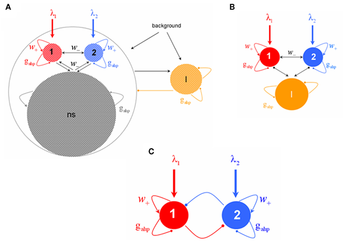
Figure 1. (A) Biophysically plausible spiking network of integrate-and-fire neurons with spike-frequency adapting mechanism based on Ca²⁺-activated K⁺ hyperpolarizing currents. There are four neuronal populations: one inhibitory (orange, I), one excitatory comprised of non-selective neurons (gray, ns), and two excitatory populations (red, 1 and blue, 2) within which neurons have similar stimulus selectivity. Arrows denote excitatory connections; lines ending to circles, inhibitory connections whereas lines ending to squares, after hyperpolarizing currents with peak conductance g_ahp. All neurons receive background input and selective populations receive an additional external stimulus λ₁, λ₂. (B) Assuming that the mean firing rate of the non-selective neuronal population is constant, the network is reduced into three neuronal populations: two excitatory (1, 2) and one inhibitory (I). (C) Four-variable reduced rate model of two populations with recurrent excitation, cross–inhibition, and neuronal adaptation.

Neurons within a certain population share the same statistical properties, i.e., single-cell parameters, inputs, and connectivity. They are modeled as leaky integrate-and-fire (LIF) neurons. The subthreshold dynamics of the membrane potential of excitatory (E) or inhibitory (I) LIF neurons is described by the following dynamics

with resting potential V_L = − 70 mV, membrane capacitance, leak conductance, and membrane time constant for excitatory neurons respectively, and for inhibitory neurons , respectively. The total synaptic current to each neuron is the sum of excitatory postsynaptic currents mediated by AMPA (I_ampa) and NMDA (I_nmda) glutamatergic and GABA_A (I_gaba) GABAergic receptors, an external excitatory postsynaptic current mediated by AMPA receptors (I_ampa,ext) and a slow Ca²⁺-activated K⁺ after-hyperpolarization current (I_ahp):

where

a = 0.5 (ms)⁻¹, δ(t) is the Dirac delta-function, and S_j are the synaptic gating variables (fractions of open channels), where sums over j are over presynaptic neurons, sums over k are over spikes emitted by the presynaptic neuron j at time and the sum over i is over spikes of the same neuron up to time t. w_j Are dimensionless connection weights between and within the neuronal populations which define the structure and function of the network. Within the selective neuronal populations excitatory synapses are potentiated by a factor w_j ≡ w ₊ > 1 according to the “Hebbian” rule according to which cells that fire together are strongly connected. In the text we refer to this factor as recurrent connectivity. Excitatory synapses between the two selective neuronal populations, and excitatory synapses between the non-selective to selective populations are modified by w_j ≡ w ₋ = 1 − f(w ₊ − 1)/(1 − f) < 1, where f = 0.15, so that the spontaneous activity of all excitatory cells is at the same level (Amit and Brunel, 1997). For the rest of the connections, w_j = 1. Reversal potentials for excitatory postsynaptic currents are V_E = 0 mV, and for inhibitory ones V_I = − 70 mV. The peak conductances for excitatory synapses are and for inhibitory where N is the total number of neurons in the network. The NMDA currents are voltage-dependent, and modulated by intracellular magnesium concentration [Mg²⁺] = 1 mM, with parameters γ = [Mg²⁺]/3.57 and β = 0.062 (mV)⁻¹. The rise time of the NMDA mediated synaptic current is τ_nmda,rise = 2 ms, while the rise time of AMPA and GABA mediated synaptic currents are neglected for being extremely fast (<1 ms). The decay time constants are τ_ampa = 2 ms, τ_nmda,decay = 100 ms, and τ_gaba = 10 ms. The reversal potential of the potassium channels is V_K = − 80 mV.

When the membrane potential of an excitatory or inhibitory neuron reaches a certain threshold V_thr = − 50 mV a spike is emitted and transmitted to other neurons. The membrane potential is reset to V_reset = − 55 mV after a refractory period, for excitatory neurons, and for inhibitory neurons. During that period the neuron is unable to produce further spikes. In addition, the gating variable Ca, emulating the cytoplasmic Ca²⁺ concentration to which we will be referring in the text, increases by a small amount ρ = 0.005, and decays exponentially with a time constant τ_Ca = 600 ms (Liu and Wang, 2001). The g_ahpCa is the effective K⁺ conductance and the g_ahp defines the level of neuronal adaptation or adaptation strength.

The total number of neurons in the network is N neurons. There are C_E = C₁ + C₂ + C_ns = 0.8N excitatory neurons, where C₁ = C₂ = fC_E neurons in each of the two selective neuronal populations, and C_ns = (1 − 2f) C_E non-selective neurons where f = 0.15. The number of inhibitory interneurons in the network is C_I = 0.2N. In order to simulate the background input, each neuron in the network receives input through C_ext = 800 excitatory connections, each one receiving an independent Poisson spike train with rate 3 Hz. To simulate the external visual stimulation, neurons within the two selective neural populations receive an additional Poisson spike train with invariant in time rates λ₁, λ₂ which define the stimuli strength.

To integrate the system of coupled differential equations that describe the dynamics of all cells and synapses we used a second order Runge–Kutta routine with a time step of 0.02 ms. To calculate the mean firing rate of a neuronal population, we divided the number of spikes emitted in a 50-ms sliding window, with a time step of 5 ms, by its number of neurons and by the window size.

Reduced Rate Model

We derived a four-variable reduced rate model from the above described spiking network, following the simplified mean-field approach of Wong and Wang (2006). This approach is based on the mean-field approximation derived in (Brunel and Wang, 2001) which analyses networks of neurons that have conductance-based synaptic inputs when the network of integrate-and-fire neurons is in a stationary state. In the mean-field approximation, it is considered the diffusion approximation according to which the sums of the synaptic gating variables (Eqs 3, 5, 7, and 10) are replaced by a DC component and a fluctuation term. Moreover, due to the different synaptic time constants, the only noise term that remains is that of the external synaptic gating variable which is considered as Gaussian. Using this approach, the original network of thousands of spiking neurons can be reduced into a set of coupled self-consistent non-linear equations. This describes the average firing rate of each neuronal population as a function of the average input current, which in turn is a function of its average firing rate. This mean-field approximation has been extended for spiking networks including Ca²⁺-activated K⁺ hyperpolarizing currents (Deco and Rolls, 2005), such as the one described in the previous section. Here, we extend the two-variable reduced model of Wong and Wang (2006) by considering this spike-frequency adaptation mechanism in neurons.

The transfer function of a LIF neuron receiving a noisy input, I_total, is given by the first-passage time formula (Renart et al., 2003):

where s is the amplitude of the fluctuations of the synaptic input, i.e., of the noise, and erf(u) is the error function. The remaining parameters have been defined in the description of the spiking network in the previous section. In the simplified mean-field approach, it is assumed that the driving force of the synaptic currents are constant and that the variance of the membrane potential does not vary significantly and it can be considered fixed as constant. Furthermore, instead of using Eq. 14, the input–output function of Abbott and Chance (2005) is considered:

where c_i (c_E = 310 (Hz/nA), c_I = 615 (Hz/nA)) is the gain factor, g_i (g_E = 0.16 s, g_I = 0.087 s) is a noise factor determining the shape of the “curvature” of ɸ, and I_i/c_i (I_E = 125 Hz, I_I = 177 Hz) is the threshold current when ɸ acts as a linear/threshold function for high g_i. The values of these parameters are calculated after fitting Eq. 15 to the first-passage time formula (Eq. 14) of a LIF excitatory (E) and of an inhibitory (I) neuron, which receives AMPA receptor-mediated external Gaussian noise (Wong and Wang, 2006).

The initial spiking network can be reduced in this way into a system with 11 + 4 variables, where the 11 are the mean firing rates of the four neuronal populations with their average synaptic gating variables. The remaining four are the average cytoplasmic Ca²⁺ concentration gating variables of the neuronal populations. While, by solving the mean-field equations, one can only determine the fixed points of the system, i.e., the stationary firing rates of the four neuronal populations describing the firing rates by the Wilson–Cowan type equations with time constant τ_r = 2 ms, one can calculate their temporal dynamics. Then, the system of the 11 + 4 variables is given by the following equations:

where i = 1, 2, ns accounts for the two selective and the non-selective to stimulus features excitatory neuronal populations, and I accounts for the inhibitory neuronal population. In Eqs 16 and 17, r_i and r_I (expressed in Hertz) are the presynaptic mean firing rate of the excitatory and inhibitory populations respectively. In Eqs 18, 20–22, and in order to be consistent with the units since the time constants are expressed in milliseconds. and stand for the average synaptic gating variables of the AMPA, NMDA, and GABA receptors respectively, and τ_ampa, τ_nmda, τ_gaba for their corresponding decay time constants. Ca_i and Ca_I stand for the cytoplasmic Ca²⁺ concentration gating variable of the three excitatory (i = 1, 2, ns), and the one inhibitory (I) population respectively. is the steady state of γ = 0.641, and (Brunel and Wang, 2001; Wong and Wang, 2006).

Furthermore, the model can be reduced to a four-variable system if we (1) assume constant activity of the non-selective neurons, (2) consider only the slow dynamics of NMDA gating variable and of the Ca²⁺-activated K⁺ channels, (3) linearize the input–output relation of the interneurons, and (4) consider the Ca²⁺ concentration gating variable of inhibitory interneurons as a function of adaptation strength. We will discuss this in more details in the following sections.

Constant activity of non-selective excitatory neurons

When there is no adaptation in the network (g_ahp = 0 nS), the firing rate of the non-selective neurons does not change much under different conditions. This allows us to assume that they fire at a constant rate of 2 Hz, as in Wong and Wang (2006). We further assume the same when there is neuronal adaptation in the network (g_ahp ≠ 0 nS) in order for our four-variable reduced model to coincide with the two-variable reduced of Wong and Wang (2006) at g_ahp = 0 nS. Implementing spike-frequency adaptation to all excitatory and inhibitory neurons, the mean firing rate of the non-selective population increases as a function of the level of neuronal adaptation, as shown in Figure 2. The mean firing rate was calculated by averaging the last 5 s of each 10 s-trial and by averaging over 100 trials. In Figure 2A, we show this dependence at different recurrent connectivities for an additional external stimulus to neurons belonging to the two selective populations of 40 Hz (a stimulus strength used in the simulations in the Results). We see that, for a given stimulus, recurrent connectivity does not change much the mean firing rate of the non-selective population as a function of the level of adaptation strength. This result stands for different stimuli (not shown here). In Figure 2B, we show the mean firing rate of the non-selective population as a function of the level of adaptation at different external inputs for a recurrent connectivity of w ₊ = 1.8 (the recurrent connectivity used in the simulations in the Results). It is apparent that there is an increase, both as a function of level of neuronal adaptation for a given stimulus, and as a function of stimulus for a given neuronal adaptation. Nevertheless, for simplicity we decided to neglect this increase and considered that the mean firing rate of the non-selective population is constant at 2 Hz for all conditions (i.e., also when there is neuronal adaptation in the network). As a consequence of this assumption, we further neglected the extra inhibition on the selective populations evoked through the interneurons. Nevertheless, as we show in Figures 7C,D and 10C,D, that the adopted assumptions do not change the results much. By assuming that the mean firing rate of the non-selective population is constant, the system is reduced to three neuronal populations as it is shown in Figure 1B.

FIGURE 2

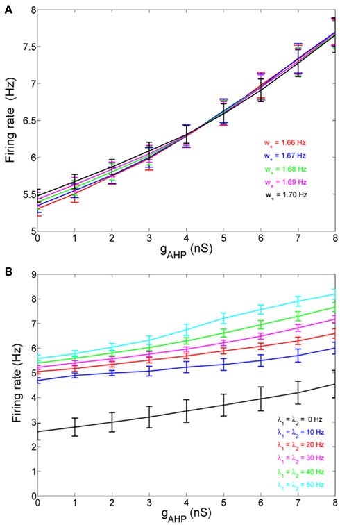
Figure 2. (A) Average firing rate of the non-selective neuronal population as a function of the level of adaptation at different recurrent connectivities for external input λ₁ = λ₂ = 40 Hz. (B) Average firing rate of the non-selective neuronal population as a function of the level of neuronal adaptation at different external stimuli for recurrent connectivity w₊ = 1.68.

Slow dynamics of NMDA gating variable and cytoplasmic Ca²⁺ concentration

The membrane time constant of LIF neurons can be neglected since they respond instantaneously to a stimulus (Brunel et al., 2001; Fourcaud and Brunel, 2002). In addition, the fast dynamics of the synaptic gating variables of AMPA and GABA_A receptors, compared to the slow synaptic gating variable of NMDA receptors, may also be neglected as they reach their steady states much faster. Their average values can thus be written as proportional to the mean firing rate of presynaptic cells (Brunel and Wang, 2001; Wong and Wang, 2006). In this work, we also consider the slow dynamics of the cytoplasmic Ca²⁺ concentration that cannot be neglected. Therefore, Eqs 19, 21, and 22 remain as they were, while Eqs 16–18 and 20 become:

where i = 1, 2. The total currents in the selective populations (1, 2) and in the inhibitory (I), resulting from the simplified mean-field approach, are given by the following equations:

where E stands for excitatory, I for inhibitory, and S₁, S₂ are the average synaptic gating variables of the NMDA receptors of the two selective populations. To the external excitatory input currents to the two selective populations, I_ampa,ext,1, I_ampa,ext,2, we included the contribution of the external stimuli (1/ms) and (1/ms) respectively. and the values of the fixed averaged membrane potentials for the excitatory and inhibitory neurons are 〈V_E〉 = − 53.4 mV, 〈V_I〉 = − 52.1 mV respectively, the same as the ones considered in Wong and Wang (2006).

Linearization of the input–output relation of interneurons

The mean firing rate of the inhibitory neurons lies in the range of 8–15 Hz when there is no spike-frequency adaptation encoded in the neurons of the network. However, when spike-frequency adaptation in all neurons in the network, the mean firing rate of the inhibitory neurons increases slightly and up to 20 Hz. Within the range 8–20 Hz, the single-cell input–output relation is still almost linear (Figure 3) and is fitted by:

FIGURE 3

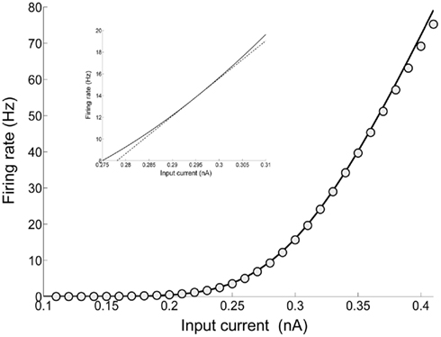
Figure 3. Input–output function of an interneuron: the line is plot of the first-passage time formula of a LIF model with σ = 4.2 (Eq. 14), while the circles correspond to the fit of Eq. 15. In the inset, a close up is drawn (solid line) and the linear approximation using Eq. 30 (dashed line).

where g_I2 = 1.7876, and r₀ = 11.3721 Hz. c_I = 615(Hz/nA) and I_I = 177 Hz are the same as in Eq. 15. By substituting I_total,I (Eq. 29) in Eq. 30 we find:

where Finally, by substituting r_I (Eq. 31) in the expressions of I_total,1(t), I_total,2(t) (Eq. 27 and 28), the system is reduced to two populations (Figure 1C).

Ca²⁺ concentration of interneurons as a function of the level of neuronal adaptation

If we consider spike-frequency adaptation to the inhibitory interneurons, the model consists of five variables, two average synaptic gating variables, S_1,2, of the selective populations, two average Ca²⁺ concentration gating variables of the selective populations, Ca_1,2, and one of the inhibitory population, Ca_I. In order to further reduce the system of equations, we assume that the Ca²⁺ concentration of the inhibitory population is constant in time at different levels of neuronal adaptation, since it changes only by a modest amount. The dependence of Ca_I on the level of neuronal adaptation is found by simulating the full biophysically plausible spiking network, as we did in Section “Constant Activity of Non-Selective Excitatory Neurons” for the mean firing rate of the non-selective population. More specifically, the Ca_I was calculated by averaging the last 5 s of each 10 s-trial, and then by averaging over 100 trials. In Figure 4A, we present Ca_I as a function of the level of neuronal adaptation at different recurrent connectivities for an additional external stimulus to both selective populations of 40 Hz (a stimulus strength used in the simulations in the Results). In Figure 4B, we present Ca_I as a function of the level of neuronal at different external inputs for a recurrent connectivity of w ₊ = 1.8 (the recurrent connectivity used in the simulations in the Results). After fitting a quadratic function to the plot Ca_I = f(g_ahp) for recurrent connectivity w ₊ = 1.68, and without external stimulus (black line in Figure 4B), we find:

FIGURE 4

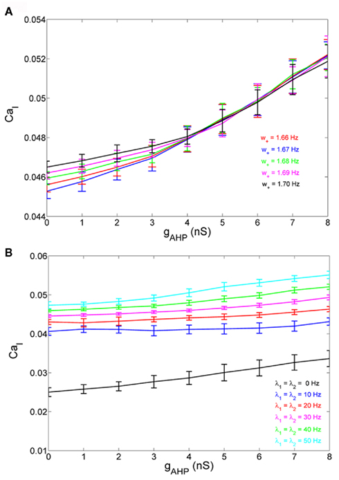
Figure 4. (A) Average gating variable Ca_I emulating the Ca²⁺ concentration of the inhibitory population as a function of the level of adaptation at different recurrent connectivities for external stimulus λ₁ = λ₂ = 40 Hz. (B) The average gating variable Ca_I as a function of the level of neuronal adaptation at different external stimuli for recurrent connectivity w ₊ = 1.68.

In Figures 4A,B, it is apparent that the shape of this function does not change significantly under different conditions, but it is shifted to higher values at higher stimuli. Nevertheless, for simplicity, we neglected this increase and we considered Eq. 32 approximated by the value 0.025 for all g_ahp, i.e. Ca_I = 0.025 for all conditions. The consequence of this assumption is that we consider higher inhibition to the selective populations. However in Figures 7C,D and 10C,D where we compare the reduced model with the spiking model, we show that both models behave similarly. We note that using Eq. 32, without approximations, we found that the final results don't change qualitatively.

Reduced four-variable model

As described in the previous sections, we consistently reduced a full biophysically plausible spiking network with spike-frequency adaptation mechanism implemented to a four-variable reduced rate model (Figure 1C). The dynamical equations characterizing this system are:

The total inward currents to the populations are given by

where

Where N is the total number of neurons in the spiking network, C_E = 0.8N, C_I = 0.2N are the numbers of the excitatory (E) and inhibitory (I) neurons, C_ext = 800 is the external excitatory connections, and f = 0.15. The rest of the parameters are: c_E = 310 (Hz/nA), g_E = 0.16 s, I_E = 125 Hz, c_I = 615 Hz/nA, I_I = 177 Hz, γ = 0.641, τ_nmda = 100 ms, τ_Ca = 600 ms ρ = 0.005, 〈V_E〉 = − 53.4 mV, 〈V_I〉 = − 52.1 mV, V_I = − 70 mV, V_K = − 80 mV, r_ext = 3 Hz, r_ns = 2 Hz, τ_ampa = 2 ms, τ_gaba = 10 ms, g_I2 = 1.7876, r₀ = 11.3721 Hz, and Ca_I = 0.025. In the present work, we used w₊ = 1.68 (w ₋ = 0.88) while g_ahp (nS) defines the level of neuronal adaptation, one of the parameters that we mainly varied.

Noise, I_noise,i where i = 1,2 stands for neuronal population 1 and 2, is modeled as white noise, filtered by the fast time constant of AMPA synapses, and described by an Ornestein–Uhlenbeck process (Uhlenbeck and Ornstein, 1930).

Where η is a Gaussian white noise with zero mean and unit variance and is the variance of the noise. In the present work, n = σ_noise defines the level of noise, and is the other parameter that we mainly varied.

Effective transfer function

It is not trivial to solve Eqs 33–40 since the mean firing rates are given by their inputs through the transfer function (Eqs 33 and 34), and the inputs are themselves dependent on the mean firing rates (Eqs 39 and 40). To overcome this difficulty of self-consistency calculations, we found (as in Wong and Wang, 2006), an effective transfer function Λ(I_total). We start by defining four variables:

Then, according to Eqs 39 and 40, in the noise-free case, Eqs 33 and 34 can be written as:

Equations 65 and 66 define a system which we can numerically solve for different sets of the variables x₁, x₂, x₃, and x₄. We then fit r₁ and r₂ with an equivalent transfer function, which depends on the new variables:

where J_A,11 = J_A,22, J_A,12 = J_A,21 and

where θ(x) is the Heaviside function. Note that the parameters a, b, d, and the function f_A are the same as in the two-variable reduced model of Wong and Wang, 2006, supplementary information D) where there is no spike-frequency adaptation in the neurons (x₃ = x₄ = 0). In that case, our four-variable reduced model coincides with the two-variable reduced model of Wong and Wang, 2006. In order to also consider spike-frequency adaptation, we included parameter e, which we approximated as linearly dependent on J_A,11 with parameters chosen to fit the numerical solutions. In Figure 5A, the average firing rate of population 1 is plotted as a function of x₁ by numerically solving Eq. 65 (line), and by fitting Eq. 67 (circles). In Figure 5B the average firing rate of population 1 is plotted as a function of x₁ for different couplings through AMPA synapses (from right to left: J_A,11 = J_A,22 = 0, 0.0005, 0.001, 0.0015 nA). As the couplings J_A,11, J_A,22 increase, the gain of the effective transfer function also does. The effective transfer functions Λ₁, Λ₂ do not change no matter how the network parameters (recurrent connectivities, synaptic conductances, stimulus strength) change.

FIGURE 5

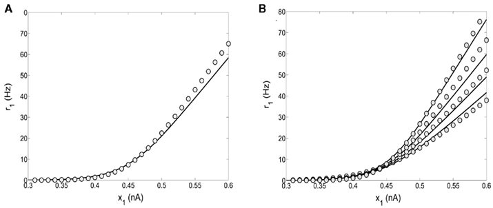
Figure 5. (A) Input–output function of population 1: the line is numerical solution of Eq. 65 and the circles are fit of the effective transfer function Eq. 67. (B) Numerical solutions (lines) and fits (circles) as in 5A for different couplings through AMPA synapses: from right to left J_A,11 = J_A,22 = 0, 0.0005, 0.001, 0.0015 nA/Hz.

Finally, our four-variable reduced rate model is given by Eqs 67, 68, 61–64, 35–38, and 60. The noise terms I_noise,1, I_noise,2 were included in the variables x₁, x₂ respectively.

Parameters and simulations

In the simulations in the Results, the recurrent connectivity weight used was w₊ = 1.68, and, hence, from Eqs 41–59, we find I₀ = 0.3553 nA, J_A,11 = J_A,22 = 9.5402 × 10⁻⁴ nA/Hz, J_A,12 = J_A,21 = 7.1258 × 10⁻⁵ nA/Hz, J_N,11 = J_N,22 = 0.1497 nA, J_N,12 = J_N,21 = 0.0276 nA, and J_A,ext = 2.2428 × 10⁻⁴ nA/Hz. The only parameter that we slightly changed is the external background input I₀, i.e., We used I₀ = 0.3536 nA in order to amplify the basin of attraction of the two unstable fixed points in the absence of stimulus and zero neuronal adaptation strength.

The mean firing rate of the two competing populations were calculated by averaging r₁ (or r₂) over a time window of 50 ms, which was sliding every 5 ms. For the numerical integration of the differential equations, we used the Euler method with a time step of 0.5 ms. The analysis of the output of the simulations is described in the Results. For the spiking simulations, we used C++ programming, for the four-variable reduced model simulations MATLAB, and for the bifurcation diagrams XPPAUT (Ermentrout, 1990).

Experimental Data

During the psychophysical experiment, subjects were presented with flickering (at 18 Hz) orthogonal sinusoidal gratings to the two eyes. The gratings (spatial frequency 2.5 cycles per degree, contrast 20%) were foveally presented on independently linearized monitors facing each other (resolution 1024 × 768 at 72 Hz). The subjects viewed the gratings through a set of angled front-surfaced silver-coated mirrors in a black shielded setup (viewing distance: 118 cm). Typically, subjects underwent 5–10 observation periods. Each observation period consisted of a rivalrous stimulation that lasted 100 s, with an interval of about 20 s between each observation period. During the rivalry period, subjects responded by pressing buttons to report the perceived orientation of the grating or released the buttons when a piecemeal pattern was perceived. Sometimes, multiple datasets were collected on different days from the same subject. From the data collected in each observation period, we calculated the mean dominance time, the coefficient of variation and gamma’s distribution parameters λ and r after fitting to the distribution of dominance periods:

where r is positive real number. Then, for each subject we averaged over all its observation periods. Mean time dominances (Td) ranged between 2.01 and 3.56 s. Coefficient of variations (CV) ranged between 0.418 and 0.704 and the gamma parameter r ranged between 2.251 and 5.446. The range of these values is what we took into account to constrain our model.

Results

In a recent study, and in order to reproduce experimental data of perceptual bistability, both noise and adaptation mechanisms were implemented in a common framework. It was shown that the working point of the model, is at the edge of the bifurcation where the system transits from noise-driven switches to adaptation-driven oscillations (Shpiro et al., 2009). Here, we come to the same conclusion with our biologically realistic reduced rate model, and we study the effect of adaptation in inhibition.

We started by considering spike-frequency adaptation to all neurons, excitatory pyramidal, and inhibitory interneurons. We found that the model replicates the experimental data in a parametric region, where both noise and neuronal adaptation contribute almost in balance. Then, we tested the same for the case where there is no spike-frequency adaptation to the inhibitory interneurons of the network. Our results show that the system still operates near the bifurcation. However, when interneurons are not adapted, a stronger level of adaptation to the excitatory neurons is necessary for the bifurcation to occur. Furthermore, adaptation of interneurons has a striking effect on the spontaneous state in the absence of stimulus. We found that in the absence of stimulus, if interneurons are adapted, the system transits to an oscillatory regime, while if interneurons are not adapted, it does not. Finally, for the parameters for which the model replicates the experimental data we show that it reproduces Levelt’s fourth and second revised proposition.

Spike-Frequency Adaptation to All Neurons of the Network

Bifurcation diagrams

In the original biologically realistic spiking neuronal network presented in the methods, all excitatory pyramidal neurons and inhibitory interneurons include spike-frequency adaptation. The reduction to the four-variable rate model was derived considering this condition. In Figures 6A,B, we show the bifurcation diagrams where the steady states of the average synaptic gating variable of one of the two neuronal populations are plotted, in the noise-free case, as a function of the level of spike-frequency adaptation, in the absence of stimulus and upon stimulus respectively. The same bifurcation diagrams stand for the other neuronal population due to symmetry in the network. Eqs 39 and 40 indicate that when interneurons include spike-frequency adaptation, there is an additional input to the selective populations due to the term:

FIGURE 6

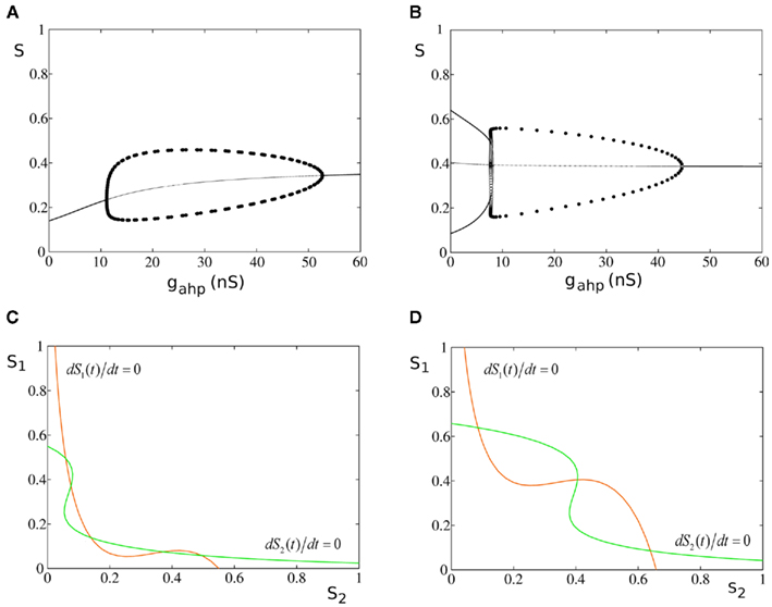
Figure 6. Spike-frequency adaptation to all neurons of the network. (A) Bifurcation diagram in the absence of stimulus. Stable steady states are represented by thick lines while unstable ones by thin lines. Filled circles are the maximum and the minimum amplitudes of stable oscillations. Open circles correspond to unstable oscillations. (B) Bifurcation diagram in the presence of stimulus λ₁ = λ₂ = 40 Hz (C). (S₁, S₂) phase-space in the absence of neuronal adaptation and in the absence of stimulus. The nullclines of the synaptic gating variables S₁ and S₂ are the green and orange lines respectively, and their intersections define the stable and unstable steady states. (D) (S₁, S₂) phase-space in the absence of neuronal adaptation but in the presence of stimulus.

In the absence of external stimulus via a supercritical Hopf-bifurcation, this additional input brings the system to a transition (at g_ahp = 11.2 nS) from a stable low firing rate regime to an oscillatory one. At a higher level of adaptation (g_ahp = 52.5 nS) the system returns to a new steady state of higher firing rate via another supercritical Hopf-bifurcation. At low levels of adaptation the steady state coexists with two stable and two unstable steady states which disappear in a fold bifurcation at g_ahp = 1.4 nS (not shown). In the bifurcation diagrams, stable steady states are represented by thick lines, and unstable ones by thin lines. The branched curves of circles show the maximum and the minimum oscillation amplitudes of one of the two selective populations when circles are filled. Open circles correspond to unstable oscillations.

In Figures 6C,D, the nullclines dS₁(t)/dt = 0, dS₂(t)/dt = 0 (whose intersections are the steady states of the system) are plotted in the (S₁, S₂) phase-space of the model, for zero spike-frequency adaptation (g_ahp = 0 nS). When neurons do not include spike-frequency adaptation, the phase-spaces of the model resemble the one of the two-variable reduced model (Wong and Wang, 2006). In the absence of stimulus, there are five fixed points (three stable and two unstable) and the system lies in the lower left fixed point where neurons fire at the same low rates (Figure 6C). When external stimulus is applied to both populations, the phase-space and the bifurcation diagram (at g_ahp = 0) reconfigure (Figures 6B,D). The input here is λ₁ = λ₂ = 40 Hz. The two asymmetrical attractors are separated by an unstable steady state (saddle node), and the system is in a bistability regime. In Figure 6B, as the level of adaptation increases, the system first transits to a mixed-mode oscillations regime (Curtu, 2010) at g_ahp = 7.7 nS and later to a stable one via two subcritical Hopf-bifurcations at g_ahp = 7.8 nS. Finally, at g_ahp = 44.5 nS, the system transits to a stable steady state via a supercritical Hopf-bifurcation.

Replicating experimental data

Keeping in mind the bifurcation diagrams, we simulated our reduced four-variable rate model by applying the same stimulation protocol as in the experiment. The input to both populations was λ₁ = λ₂ = 40 Hz. For each level of neuronal adaptation, i.e., peak conductance of the Ca²⁺-activated K⁺ channels, g_ahp, we applied this stimulus for 100 s. We then calculated the mean Td of the two percepts, and the coefficient of variation. After fitting the distribution of Td to a gamma distribution, we calculated the parameter r (Eq. 74). In order to mimic the experimental protocol that each subject underwent, for each g_ahp, we performed 10 such trails, and computed the average values of mean Td, the coefficient of variation and the r parameter from the gamma distribution fit over these trials. Finally, we did the same with different levels of noise. One dominance period was defined as the time starting when the difference in the firing rates of the two populations was 5 Hz and ended when it became zero. In Figure 7A, we present the mean Td, and the coefficient of variation for five levels of noise as a function of neuronal adaptation, g_ahp. In Figure 7B, the r parameter from the gamma distribution fit is plotted as a function of level of neuronal adaptation and for the same levels of noise. The horizontal lines denote the range that the experimental data define. Vertical lines in Figures 7A,B are drawn at the bifurcation points where the system transits from a bistable dynamical regime to an oscillatory one, as presented in the corresponding bifurcation diagram (Figure 6B). We are looking for the level of noise and of adaptation at which the model results reside in the range of values defined by the experimental data. The green big circle denotes such levels (g_ahp = 6.2 nS, n = 0.016), and in Figure 7C, we plot the mean firing rates of both populations at these levels in the absence (black and green plots) and upon (blue and red plots) stimulus. For these parameters, the mean Td = 3.24 s, the coefficient of variation is CV = 0.457, and r = 2.841.

FIGURE 7

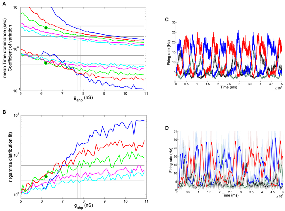
Figure 7. Spike-frequency adaptation to all neurons of the network: Replicating the experimental data (A) Mean time dominance and coefficient of variation as a function of neuronal adaptation for different levels of noise (blue: n = 0.01, red: n = 0.014, green: n = 0.016, magenta: n = 0.018 and celestial: n = 0.019) for λ₁ = λ₂ = 40 Hz. (B) Parameter r of gamma distribution fit to the distribution of dominance times as a function of neuronal adaptation for the same noise levels as in (A). In both (A,B), horizontal lines denote the range that the experimental data define. Vertical lines are drawn at the bifurcation points where the system transits from a bistable dynamical regime to a mixed-mode oscillations and to an oscillatory regime. Green big circles at the levels g_ahp = 6.2 nS, n = 0.016 indicate a case where the model replicates the experimental data. We find that the model replicates the experimental data in the noise-driven regime and close to the bifurcation. (C) The mean firing rate of the selective populations for g_ahp = 6.2 nS and n = 0.016 in the absence of stimulus (black and green plots) and upon stimulus (blue and red plots). (D) The mean firing rate of the selective neuronal populations by simulating the spiking network (with N = 500 neurons) with the same parameters as the ones used simulating the reduced model (C). Thin lines are plots from a trial and thick lines are the same after smoothing. We see that both models exhibit similar behavior in both the presence (blue and red plots) and absence (black and green plots) of the stimulus.

From our results, it is apparent that both noise and adaptation are the driving forces for the alternations in BR. The working point of our model is in the bistability regime and close to the bifurcation toward the oscillatory. Noise and adaptation contribute almost in balance to the perceptual alternations. At this point, we should note that the level of noise necessary for the model to replicate the experimental data is high enough to drive the system into the oscillatory regime (Figure 6A) in the absence of stimulus as one can see in Figure 7C (black and green plots).

Moreover, in Figure 7D, we plot the mean firing rates of the selective neuronal populations as we compute them by simulating the spiking network with N = 500 total neurons, and with the same parameters we used to plot Figure 7C. Thin red and blue plots correspond to the activity of the selective populations upon stimulus, and thin black and gray plots to their activity in the absence of stimulus, while thick plots are the corresponding activity after smoothing with a time window of 500 ms (sliding every 50 ms). We see that both the spiking and the reduced model exhibit similar behavior in the presence, as well as in the absence, of the stimulus. This means that the approximations we considered for the derivation of our four-variable reduced rate model (see Materials and Methods) are accurate. In addition, for these parameters, we ran 10 trials of 100 s-stimulation. From the smoothed mean firing rates, we computed the average mean Td, coefficient of variation, and r parameter from the gamma distribution fit to the distribution of the Td at each of the 10 trials, as we did with the reduced model. We found mean Td = 2.82 s, mean coefficient of variation CV = 0.582 and r = 3.137. These values reside in the range defined by the experimental data, similarly as we found with the reduced model. Finally we computed the bifurcation point, where the model transits to the mix-mode oscillatory regime, employing the spiking network. The total number of neurons used was N = 20000 in order to decrease the noise in the network as much as possible. The bifurcation point is at g_{ahp,bif,spiking} = 6 nS, close to the bifurcation point found with the reduced model (g_{ahp,bif,reduced} = 7.7 nS). The g_{ahp,bif,reduced} is higher than the g_{ahp,bif,spiking} due to the assumptions adopted in the Methods but mostly to the advantage of the reduced model to eliminate noise which cannot be done in the spiking network.

Furthermore, we tested the effect of increasing the external stimulus strength (λ₁ = λ₂ = 50 Hz) which would correspond to an increase of the stimulus contrast in the experiment. The rest of the parameters were the same as before, as well as the stimulation protocol and analysis. In Figures 8A,B (thick lines), we present the results for the same levels of noise, as in Figures 7A,B. We also plot the results for λ₁ = λ₂ = 40 Hz (thin lines) for comparison. Levelt’s fourth proposition indicates that increasing the stimulus contrast results in an increase of the average rivalry reversal rate (Levelt, 1968), which corresponds to a decrease in the average dominance duration. This is apparent in Figure 8A for all levels of neuronal adaptation and of noise. In addition, by increasing the strength of the external stimulation, the bifurcation points (vertical lines) shift to lower values, while the mixed-mode oscillations regime narrows. Nevertheless, the model’s results (Td = 2.49 s, CV = 0.457, and r = 2.825) reside again in the ranges defined by the experimental data, while working in the bistable regime (big red circle: g_ahp = 5.4 nS, n = 0.014) and close to the bifurcation point g_{ahp,bif,reduced} = 5.8 nS. Once more, for the same parameters, we simulated the spiking network (with N = 1000 neurons), and found Td = 3.298 s, CV = 0.462, and r = 3.975. These values are close to the ones computed with the reduced model and inside the range of the experimental data. The bifurcation point as calculated by simulating the spiking network with N = 20000 total neurons, is at g_{ahp,bif,spiking} = 4.3 nS.

FIGURE 8

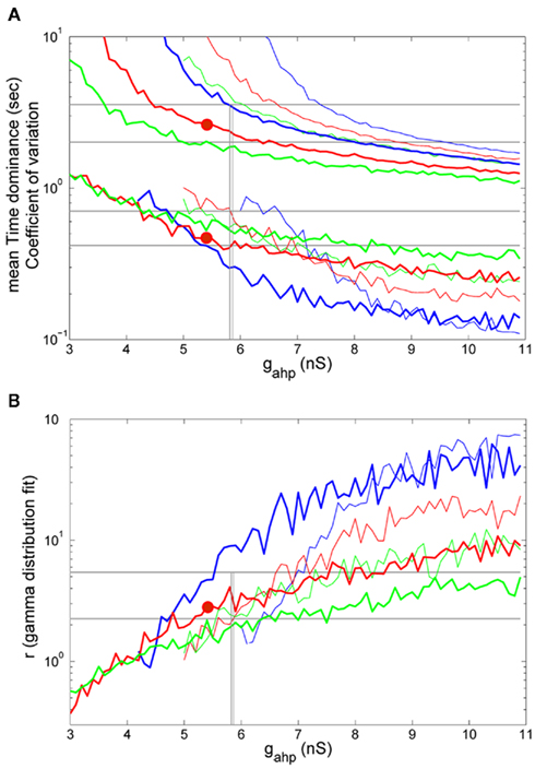
Figure 8. (A) Mean time dominance and coefficient of variation as a function of neuronal adaptation for different levels of noise (blue: n = 0.01, red: n = 0.014 and green: n = 0.016) for λ₁ = λ₂ = 40 Hz (thin lines) and λ₁ = λ₂ = 50 Hz (thick lines). (B) Parameter r of gamma distribution fit to the distribution of dominance times as a function of neuronal adaptation for the same levels of noise as in (A). In both (A,B), horizontal lines denote the range that the experimental data define. Vertical lines are drawn at the bifurcation points where the system transits from a bistable dynamical regime to a mixed-mode oscillations and to an oscillatory regime. Red big circles at g_ahp = 5.4 nS, n = 0.014 indicate a case for which the model replicates the experimental data.

Spike-Frequency Adaptation Only to the Excitatory Pyramidal Neurons of the Network

Bifurcation diagrams

We removed neuronal adaptation from interneurons by setting κ = 0 in Eqs 63 and 64. The rest of the parameters of the model remained the same. We note that when interneurons are not adapted, the mean firing rate of the non-selective population and the mean firing rate of the inhibitory population decrease for higher adaptation strengths. Here, we again assume that the mean firing rate of the non-selective population is constant in all conditions, as we had assumed in the case of adapted interneurons (see Constant Activity of Non-Selective Excitatory Neurons of Materials and Methods). In addition, and for simplicity, we kept the same parameters of the linearization of the input–output formula (Eq. 30) as in the case of adapted interneurons. In the following we show that these assumptions do not change the results much.

In Figure 9, we present the bifurcation diagram of one of the two neuronal populations in the absence and in the presence of an external stimulus employing our four-variable reduced rate model. The same bifurcation diagrams also stand for the other population due to symmetry. While in the presence of a stimulus, the bifurcation diagram (Figure 9B) is qualitatively similar as in the case where we included spike-frequency in interneurons (Figure 6B), the bifurcation diagram is qualitatively different in the absence of external stimulus (Figure 9A compared to Figure 6A). Here, there is no additional input (Eq. 75) to the excitatory populations and the system remains in a stable steady state of low firing rate which decreases as level of neuronal adaptation increases (Figure 9A). We note that, as in the case where all neurons are adapted, at low levels of adaptation the steady state coexists with two stable and two unstable steady states which disappear in a fold bifurcation at g_ahp = 0.36 nS (not shown).

FIGURE 9

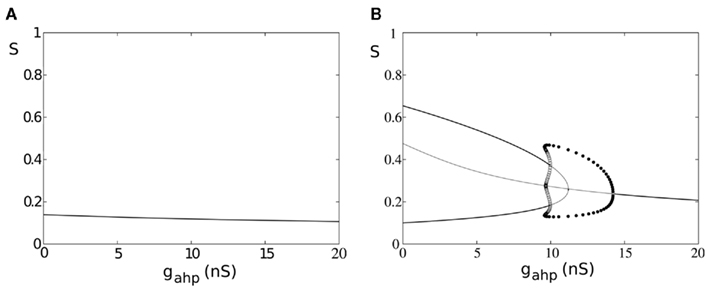
Figure 9. Spike-frequency adaptation only to the excitatory pyramidal neurons of the network. (A) Bifurcation diagram in the absence of stimulus, stable steady states are represented by thick lines while unstable ones by thin lines. Filled circles are the maximum and the minimum amplitudes of stable oscillations. Open circles correspond to unstable oscillations. (B) Bifurcation diagram in the presence of stimulus λ₁ = λ₂ = 50 Hz.

In Figure 9B, stable steady states are represented by thick lines, and unstable ones by thin lines. Filled circles correspond to the maximum and minimum values of stable oscillations, while open circles correspond to unstable oscillations. Upon stimulus presentation, λ₁ = λ₂ = 50 Hz, and at g_ahp = 0, the system transits from a stable steady state of low firing rate to a winner-take-all regime, where one of the populations fires at high rate while the other fires at low rate. The system reaches the attractor and lies in a bistability regime. Without noise, the system would remain in this attractor, being unable to transit to its anti-symmetrical (i.e., switches in perception are not possible). As adaptation increases, the basin of attraction decreases, and switches are more likely to occur upon noise introduction. Nevertheless, higher levels of adaptation drive the system into an oscillatory regime where, even in the absence of noise, alternations from one percept to the other are inevitable. More specifically, starting at high values of g_ahp, the system lies in a stable steady state where both populations fire at low firing rate. As g_ahp decreases, the system transits to a stable oscillatory regime via a supercritical Hopf-bifurcation at g_ahp = 14.2 nS. At g_ahp = 9.96 nS, the system transits into a mixed-mode oscillations regime (Curtu, 2010) via two subcritical Hopf-bifurcations. The big unstable periodic orbit coalesces with the stable periodic orbit at g_ahp = 9.57 nS, via a double limit cycle bifurcation, and the system transits to the bistability regime where two anti-symmetric attractors are separated by a saddle node fixed point. At g_ahp = 11.2 nS, the trajectories of the three unstable fixed points coalesce into an unstable fixed point via a subcritical pitch-fork bifurcation. This cumbersome dynamics of the mixed-mode oscillations regime, although very interesting, is beyond the scope of the present study. The dynamics of our model has similar characteristics as described in Shpiro et al. (2007), Curtu et al. (2008), Curtu (2010). A point to note is that, in our case, we also have recurrent excitation resulting in an asymmetry between regimes of release and escape mechanisms with the release regime being small due to the recurrent connectivity in the network (Shpiro et al., 2007; Seely and Chow, 2011).

Replicating experimental data

We saw previously that when inhibitory interneurons are adapted, both noise and adaptation are responsible, almost in balance, for the perceptual alternations. Here, we follow the same stimulation protocol and analysis, as in Section “Replicating Experimental Data,” for the case where inhibitory interneurons are not adapted. With the bifurcation diagram (Figure 9B) in mind, we applied the same fixed external stimulus to both populations, λ₁ = λ₂ = 50 Hz. We then computed the mean Td, the coefficient of variation and the r parameter of the gamma distributions fit to the distributions of dominance times, as a function of neuronal adaptation, at different levels of adaptation and of noise. The rest of the parameters are the same except for the exclusion of spike-frequency adaptation from interneurons by setting κ = 0 in Eqs 63 and 64. The results are presented in Figure 10. Different lines correspond to different noise levels. Horizontal lines denote the range that the experimental data define. Vertical lines are drawn at the bifurcation points which define the different dynamical regimes.

FIGURE 10

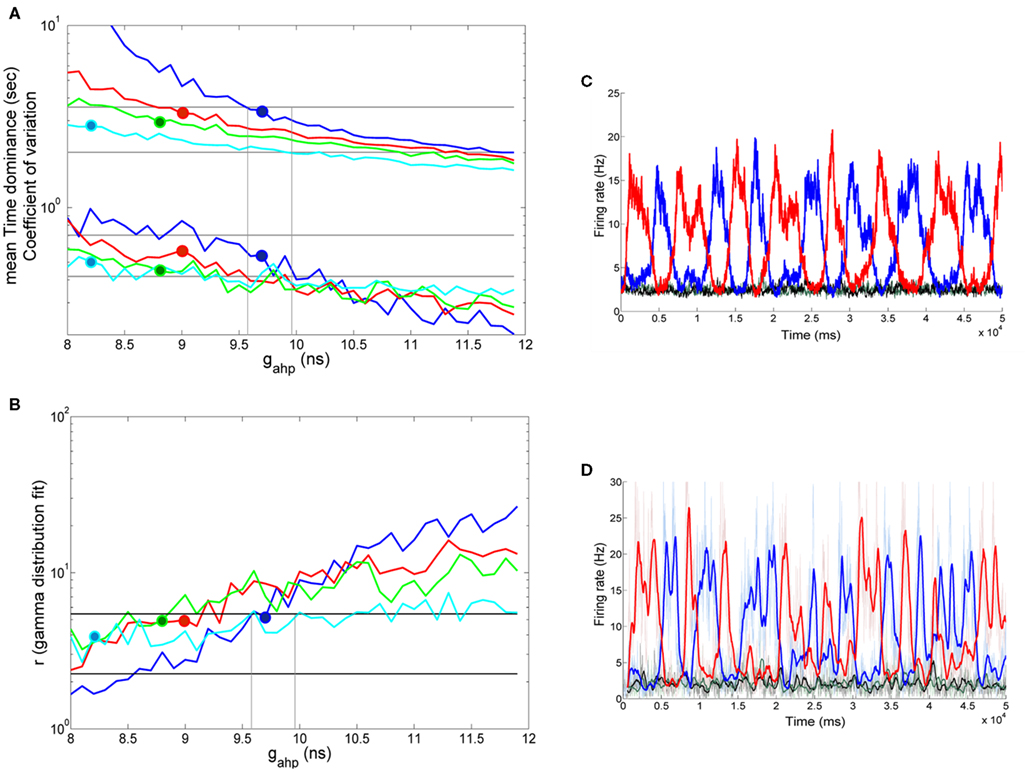
Figure 10. Spike-frequency adaptation only to the excitatory pyramidal neurons of the network: Replicating the experimental data. (A) Mean time dominance and coefficient of variation as a function of neuronal adaptation for different levels of noise (blue: n = 0.01, red: n = 0.014, green: n = 0.016, and celestial: n = 0.019) for λ₁ = λ₂ = 50 Hz. (B) Parameter r of gamma distribution fit to the distribution of dominance times as a function of neuronal adaptation for the same levels of noise as in (A). In both (A,B), horizontal lines denote the range that the experimental data define. Vertical lines are drawn at the bifurcation points where the system transits from a bistable dynamical regime to a mixed-mode oscillations and to an oscillatory regime. Blue, red, green, and celestial big circles at g_ahp = 9.7 nS, g_ahp = 9 nS, g_ahp = 8.8 nS, and g_ahp = 8.2 nS, respectively indicate sets of parameters for which the model replicates the experimental data. We find that the model operates in the bistability regime close to the bifurcation as well as in the mixed-mode oscillation regime (blue big circle). (C) The mean firing rate of the populations for g_ahp = 9 nS and n = 0.014 in the absence of stimulus (black and green plots) and upon stimulus (blue and red plots). (D) The mean firing rate of the selective neuronal populations by simulating the spiking network (with N = 500 neurons) with the same parameters as the ones used in (C). Thin lines are plots from a trial, and thick lines are the same after smoothing. We see that both models exhibit similar behavior in both the presence (blue and red plots) and in the absence (black and green) of the stimulus.

In Figures 10A,B, big blue (g_ahp = 9.7 nS, n = 0.01), red (g_ahp = 9 nS, n = 0.014), green (g_ahp = 8.8 nS, n = 0.016), and celestial (g_ahp = 8.2 nS, n = 0.019) circles are sets of parameters for which all three mean Td, coefficient of variation, and r parameter reside in the range defined by the experimental data. We find that, in all these cases, the model is in the bistability regime and near to the bifurcation point. We note that it is also possible that for a given noise-level (n = 0.01, blue big circle), experimental data are replicated inside the mixed-mode oscillations regime. In Figure 10C, we plot the mean firing rates of the two neuronal populations when level of noise is n = 0.014, and adaptation strength is g_ahp = 9 nS (red big circle in Figures 10A,B) in two conditions: in the absence of stimulus (black and green plots) and upon stimulus (blue and red plots). We see that when interneurons are not adapted neuronal populations fire at low rates and in an asynchronous state in the absence of stimulus.

Moreover, in Figure 10D, we plot the mean firing rates of the two selective neuronal populations, as we compute them by simulating the spiking network with N = 500 total neurons, and with the same parameters we used to plot Figure 10C. As in the case where we considered adapted inhibitory interneurons (Figures 7C,D), both models behave similarly in the presence and in the absence of the stimulus, indicating that the assumptions adopted for the reduction are accurate. In addition, we computed the mean Td, the coefficient of variation and the r parameter from the gamma distribution fit to the distribution of the Td simulating the spiking network (as we did in section Replicating Experimental Data). We found that the results were in the range defined by the experimental data. More specifically, we found Td = 2.64 ms, CV = 0.463, and r = 5.147, similar to the ones we attained with the reduced model for the same parameters (Td = 3.29 ms, CV = 0.581, and r = 4.992). Finally, we computed the bifurcation point by simulating the spiking network with N = 20000 neurons, and we found that the bifurcation point is at g_{ahp,bif,spiking} = 8.3 nS, close to the bifurcation point we observed with the reduced model (g_{ahp,bif,reduced} = 9.57 nS). As in the case where inhibitory interneurons are also adapted, the g_{ahp,bif,reduced} is higher than the g_{ahp,bif,spiking}. This is a consequence of the assumptions adopted for the derivation of the reduced model, as well as of the noise in the spiking network which cannot be totally eliminated.

Furthermore, in Figure 11, we plot the mean Td and the coefficient of variation for the two extreme cases, i.e., all interneurons are all (gray lines) or none (black lines) adapted. We plot the results from the simulations where in both cases the stimulus strength is λ₁ = λ₂ = 50 Hz and the level of noise is n = 0.014. We see that by removing spike-frequency adaptation mechanism from interneurons, mean dominance duration and its coefficient of variation increase for the same level of neuronal adaptation to the excitatory neurons. The bifurcation points, where the model transits from noise-driven switches to adaptation-driven oscillations, shifts to higher values of g_ahp. At the same time, the level of adaptation for which the model replicates the experimental data also increases but resides in both cases within the bistability regime and close to the bifurcation.

FIGURE 11

Figure 11. Mean time dominance and coefficient of variation as a function of neuronal adaptation for level of noise n = 0.014, when inhibitory interneurons are adapted (gray lines) and when they are not adapted (black lines) for stimulus strength λ₁ = λ₂ = 50 Hz. Gray and black vertical lines define the bifurcation points when inhibitory interneurons are adapted and when they are not, respectively.

Levelt’s Second Revised and Fourth Proposition

Levelt’s four propositions in BR (Levelt, 1968) exemplify how stimulus parameters affect the duration of perception of two conflicting images. These propositions define additional constrains to computational models candidates to explain BR. Most of the times, computational models were tested with Levelt’s second and fourth proposition. Recently, Levelt’s second proposition has been revised (Brascamp et al., 2006) and states that, when the contrast of one image changes the average dominance duration of the image with higher contrast is mainly affected. Levelt’s fourth proposition states that when the contrast of both images increases, the average rivalry reversal rate increases, meaning that the mean Td of both images decreases.

Here, we tested Levelt’s second revised proposition for four sets of noise and neuronal adaptation levels (big blue, red, green, and celestial circles in Figures 10A,B) for which the model’s results reside in the ranges defined by the experimental data, when inhibitory interneurons are not adapted. The results are shown in Figures 12A–C. In the insets, we tested the same for the case where inhibitory interneurons are adapted with the same level of noise and stimulus strength (big red circle, Figures 8A,B) as when they are not adapted. We first applied equal stimulus for 100 s to both populations of low strength, λ₁ = λ₂ = 45 Hz. We then computed the mean dominance durations of each population and we averaged over 10 such trials. Then, we kept the stimulus to one of the populations fixed, λ₁ = 45 Hz, and we increased the other. The results are shown in Figure 12A. In Figure 12B, we applied equal stimulus of intermediate strength to both populations, λ₁ = λ₂ = 47.5 Hz, and we computed the mean Td as previously. Then, we kept the stimulus to one population fixed, λ₁ = 47.5 Hz, and we manipulated the other. Finally, we applied equal stimulus of high strength to both populations, λ₁ = λ₂ = 50 Hz, and computed the mean dominance periods. Then, we kept the stimulus to one of the populations fixed at this high level, λ₁ = 50 Hz, while we decreased the other (Figure 12C). In Figures 12A–C, the dashed lines are plots of the mean Td of the population receiving fixed stimulus (λ₁) while solid lines are plots of the mean Td of the population receiving variable stimulus (λ₂). Vertical lines denote the stimulus strength when it is equal to both populations. We see that Levelt’s second revised proposition is satisfied by all four levels of neuronal adaptation and noise for which our model replicates the experimental data when inhibitory interneurons are not adapted as well as when they are (insets in Figures 12A–C). We should mention though that from Moreno-Bote et al. (2010), we know that alternation rate is higher and symmetric around equi-dominance, i.e., when external stimulus is equal to both neuronal populations. This would be an additional constrain for the model. In Figure 12B, we see that this is not always the case. Nevertheless, in the study by Moreno-Bote et al. (2010), it is shown that models best replicate this result when normalized stimuli are applied, which is not the case here.

FIGURE 12

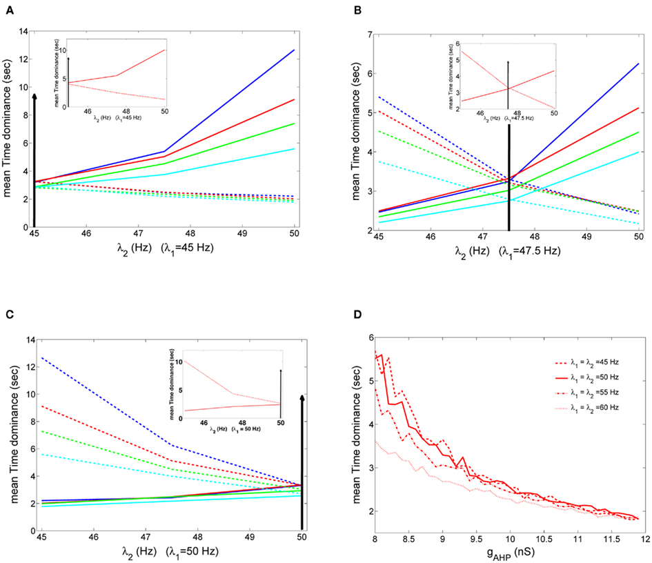
Figure 12. (A–C) Mean time dominance of one of the two neuronal populations of the model receiving fixed stimulus λ₁ (dashed lines) and of the neuronal population receiving variable stimulus λ₂ (solid line), as a function of the variable external stimulus λ₂, for the four noise-adaptation points for which the model replicates the experimental data when interneurons are not adapted (big circles in Figures 10A,B). Arrows denote the starting point where both populations receive the same stimulus, λ₁ = λ₂. In the insets the same are plotted for the case where inhibitory interneurons are adapted (red big circle in Figures 8A,B). A: when λ₁ = 45 Hz, (B) when λ₁ = 47.5 Hz and (C) when λ₁ = 50 Hz. (D) Mean time dominance of both populations for different stimulus strengths when inhibitory interneurons are not adapted and n = 0.014.

In Section “Replicating Experimental Data,” we tested Levelt’s fourth proposition for two different stimulus strengths in the case where inhibitory interneurons are adapted. Here, we test Levelt’s fourth proposition for the case where inhibitory interneurons are not adapted for applied stimulus strengths λ₁ = λ₂ = 50,50,55,60 Hz (Figure 12D). Each stimulation lasted 100 s, and at each trial we computed the mean dominance durations of both populations. Finally, we averaged over 10 trials. The level of noise was n = 0.014. In Figure 12D, we see that as stimulus strength increases mean dominance duration decreases. Thus our model accounts for Levelt’s fourth proposition. Note that this decrease is more prominent at low levels of neuronal adaptation and at higher levels of neuronal adaptation mean Td is similar across different stimulus strengths.

Discussion

In the present work, we present a theoretical approach which could provide novel insights into the microcircuit dynamics responsible for multistable perception. We consistently derived a four-variable reduced rate model from a biologically plausible spiking neuronal network, and we tested it considering experimental behavioral data of BR. We calculated the mean dominance duration of the percepts, the coefficient of variation, and the parameters of the gamma distribution fit to the distribution of dominance durations. We emulated the experiment by simulating our reduced model for different sets of noise and neuronal adaptation levels, and we looked for the optimal ones for which the model replicates the experimental data. In the noise-free condition, the range of adaptation strength defines different dynamical regimes where our model can operate. There is a bistability regime, where switches can only arise due to the implementation of noise. There is a mixed-mode oscillations regime which is the transition regime of the model from the bistability to the oscillatory regime. Finally, there is an adaptation-driven oscillatory regime where alternations can happen even without noise. By testing different levels of noise and adaptation strengths, we came to the same conclusion as Shpiro et al. (2009). In order to satisfy the experimental data, the system must operate in the noise-driven regime close to the boundary with the adaptation-driven regime. Thus, both mechanisms are responsible in balance for the perceptual alternations.

It is not the first time that a reduced spiking model is used to explain BR. Laing et al. (2010) recently presented reduced rate-like models derived from a fine scale spiking model consisting of two populations, one excitatory and one inhibitory, of Hodgkin–Huxley type neurons (Laing and Chow, 2002). Neurons are orientation selective, include both spike-frequency adaptation and synaptic depression, and each population can be thought of as lying on a ring. Nevertheless, their reduction is not derived consistently from the spiking network. Instead it is based on both intuition based on observations of the spiking network, and on data-mining tools to select appropriate variables. By processing the results of simulations, the authors determined functions that govern the dynamics of these variables. Our reduced model, on the other hand, is consistently derived from a spiking network using mean-field techniques. In addition, we studied the underlying mechanism responsible for perceptual alternations as Shpiro et al. (2009), and we extended the results by studying the effect of adapting inhibitory interneurons.

The biophysically realistic spiking network, from which we derived the reduced model, has been previously studied for perceptual bistability (Moreno-Bote et al., 2007). Their spiking network is very similar to ours, but the main difference is that they only include spike-frequency adaptation to excitatory pyramidal cells. Their interesting results show the effect of noise and stimulus strength in the behavior of the network. The novelty of our work is that we implemented a four-variable reduced rate-like model which we derived consistently from a similar biophysically realistic spiking network of thousands of neurons using mean-field techniques. More specifically, we performed a further reduction of the extended mean-field model (Deco and Rolls, 2005). This helps us understand the dynamics of the full original spiking network, which in turn can provide us with numerous data such as realistic synaptic dynamics, spiking time series, local field potentials, etc.

Moreover, we were able to study two extreme cases by including spike-frequency adaptation in all or in none of the network’s inhibitory interneurons. Interestingly, we found that, in both cases, our model replicates the experimental data in the boundary between noise and adaptation. We thus conclude that spike-frequency adaptation of inhibitory interneurons is not relevant to the cause of perceptual alternations observed in BR. However, we demonstrate that adaptation of interneurons has an effect on the parametric space where the bifurcation is observed. When interneurons are not adapted, stronger adaptation is necessary in the remaining components of the network to induce a bifurcation. As a result, more adaptation is necessary to obtain the optimal working point of the system.

Additionally, we found that spike-frequency adaptation in interneurons generates different types of spontaneous dynamics. When the interneurons in the spiking network are not adapted, the selective neuronal populations fire asynchronously and at low rates during the spontaneous state. On the other hand, when interneurons are adapted, the model exhibits an oscillatory regime even during the spontaneous state. This type of oscillatory regime has been reported in an attractor memory network (Lundqvist et al., 2010). Here, for the set of parameters for which the model replicates the experimental data, noise is high enough to drive the system into the oscillatory regime in the absence of stimulus, when interneurons are adapted.

Furthermore, adapted inhibitory interneurons affect the reaction time at the onset of a stimulus. In Theodoni et al. (2011), it has been shown that neuronal adaptation accelerates decisions in an adaptation-related aftereffects decision making task. The spiking model studied in that work is similar to the one presented here (when all inhibitory interneurons are adapted). From our four-variable reduced model, we found that when interneurons include spike-frequency adaptation, an additional input to both selective populations is implemented which increases with adaptation strength. This results in a faster ramping activity at higher adaptation strengths, which in turn leads to faster reaction times at the onset of a stimulus. We expect that when interneurons are not adapted, we would have the opposite effect.

We would like to note that we examined two extreme conditions. Either all the inhibitory interneurons of the network are adapted or none of them. Nevertheless, for example in the prefrontal cortex, where neuronal activity follows phenomenal perception (Panagiotaropoulos et al., unpublished data), we know that there are three types of interneurons. Half of them are dendritic-targeting, and the others are divided into interneurons targeting, and perisoma targeting (Conde et al., 1994; Gabbott and Bacon, 1996). Perisoma targeting interneurons do not include spike-frequency adaptation while the rest do include (Wang et al., 2004). In our network neurons are not considered as multi-compartmental, and we cannot distinguish the inhibitory interneurons among these three types. Nevertheless, a more biophysically plausible condition would be to consider a percentage of adapted inhibitory interneurons.

Levelt’s propositions show how mean dominance durations are affected as a function of stimulus strength to both or to one eye. They refer to BR but it has been shown that there is a general validity in other paradigms of visual rivalry, revealing common computational mechanisms (Klink et al., 2008). Levelt’s propositions, especially the second and the fourth, have been a usual constrain for computational models of BR (Laing and Chow, 2002; Brascamp et al., 2006; Moreno-Bote et al., 2007, 2010; Wilson, 2007; Seely and Chow, 2011). In the present work, we tested Levelt’s fourth proposition in both conditions, where interneurons are all or none adapted. In both conditions, we found that the reduced model satisfies this law. In addition we tested Levelt’s second revised proposition (Brascamp et al., 2006), and found that the model also satisfies this law. We would like to mention that our study was not in full accordance with the recent study of Moreno-Bote et al. (2010). They showed that competition models like ours better reproduce experimental findings based on Levelt’s revised second proposition when the stimuli applied to the populations are normalized, which was not the case in the present work.

In addition, we note that, in this study, we did not check for serial correlations in percept durations. Interestingly, non-zero serial correlations were reported recently in both BR and structure-from motion ambiguity paradigms (van Ee, 2009). Experimental findings in their work were replicated by implementing noise in adaptation of percept-related neurons. It would be interesting to see whether our reduced model can reproduce such serial correlations, and in what conditions. Furthermore, an open and interesting question is the freezing of perception during intermittent presentation of ambiguous stimuli (Orbach et al., 1963; Leopold et al., 2002; Maier et al., 2003). Using a reduced model consistently derived from a biologically realistic spiking network one could study the underlying dynamics, and may unravel mechanisms underlying such a phenomenon.

Lastly, BR has often been compared to cognitive processes such as attention and decision making (Leopold and Logothetis, 1999; Stoner et al., 2005). But it is only recently, that attempts have been made to study how these phenomena might be related (Braun and Mattia, 2010; Kalisvaart et al., 2011) within a theoretical framework. We have used a biophysically realistic spiking network that was initially used to model working memory (Brunel and Wang, 2001) and later decision making (Wang, 2002), attention (Deco and Rolls, 2005), and adaptation-related aftereffects in perceptual decisions (Theodoni et al., 2011). The ability of a similar spiking network to produce these different, but related, cognitive phenomena indicates that they could have similar underlying neural mechanisms.

Conflict of Interest Statement

The authors declare that the research was conducted in the absence of any commercial or financial relationships that could be construed as a potential conflict of interest.

Acknowledgments

The authors would like to thank KongFatt Wong, Antoni Guillamon, James Rankin, Robert Ton, for their useful communications, and Tristan Nakagawa for his comments on the manuscript. The research leading to these results has received funding from the European Community’s Seventh Framework Programme FP7/2007-2013 under grant agreement number 214728-2, and the Max Planck Society. It was also supported by the European Union grant “Brainsynch” and “BrainScaleS” by the Spanish Research Project SAF2010-16085, and by the CONSOLIDER – INGENIO 2010 Programme CSD2007-00012.

References

Abbott, L. F., and Chance, E. S. (2005). Drivers and modulators from push-pull and balanced synaptic inputs. Prog. Brain Res. 149, 147–155.

Pubmed Abstract | Pubmed Full Text | CrossRef Full Text

Alais, D., Cass, J., O’Shea, R. P., and Blake, R. (2010). Visual sensitivity underlying changes in visual consciousness. Curr. Biol. 20, 1362–1367.

Pubmed Abstract | Pubmed Full Text | CrossRef Full Text

Amit, D. J. (1995). The hebbian paradigm reintegrated: local reverberations as internal representations. Behav. Brain Sci. 18, 617–625.

CrossRef Full Text

Amit, D. J., and Brunel, N. (1997). Model of global spontaneuous activity and local structured activity during delay periods in the cerebral cortex. Cereb. Cortex 7, 237–252.

Pubmed Abstract | Pubmed Full Text | CrossRef Full Text

Blake, R. (1989). A neural theory of binocular rivalry. Psychol. Rev. 96, 145–167.

Pubmed Abstract | Pubmed Full Text | CrossRef Full Text

Blake, R. (2001). A primer on binocular rivalry. Brain Mind 2, 5–38.

CrossRef Full Text

Blake, R., and Logothetis, N. K. (2002). Visual competition. Nat. Rev. Neurosci. 3, 13–21.

Pubmed Abstract | Pubmed Full Text | CrossRef Full Text

Brascamp, J. W., van Ee, R., Noest, J. A., Jacobs, R. H. A. H., and van den Berg, A. V. (2006). The time course of binocular rivalry reveals a fundamental role of noise. J. Vis. 6, 1244–1256.

Pubmed Abstract | Pubmed Full Text | CrossRef Full Text

Braun, J., and Mattia, M. (2010). Attractors and noise: twin drivers of decisions and multistability. Neuroimage 52, 740–751.

Pubmed Abstract | Pubmed Full Text | CrossRef Full Text

Brunel, N., Chance, F. S., Fourcaud, N., and Abbott, L. F. (2001). Effects of synaptic noise and filtering on the frequency response of spiking neurons. Phys. Rev. Lett. 86, 2186–2189.

Pubmed Abstract | Pubmed Full Text | CrossRef Full Text

Brunel, N., and Wang, X.-J. (2001). Effects of neuromodulation in a cortical network model of object working memory dominated by recurrent inhibition. J. Comput. Neurosci. 11, 63–68.

Pubmed Abstract | Pubmed Full Text | CrossRef Full Text

Conde, F., Lund, J. S., Jacobowitz, D. M., Baimbridge, K. G., and Lewis, D. A. (1994). Local circuit neurons immunoreactive for calretinin, calbindin D-28k or parvalbumin in monkey prefronatal cortex: distribution and morphology. J. Comp. Neurol. 341, 95–116.

Pubmed Abstract | Pubmed Full Text | CrossRef Full Text

Curtu, R. (2010). Singular Hopf bifurcations and mixed-mode oscillations in a two-cell inhibitory neural network. Physica D 239, 504–514.

CrossRef Full Text

Curtu, R., Shpiro, A., Rubin, N., and Rinzel, J. (2008). Mechanisms for frequency control in neuronal competition models. SIAM J. Appl. Dyn. Syst. 7, 609–649.

Pubmed Abstract | Pubmed Full Text | CrossRef Full Text

Deco, G., and Rolls, E. T. (2005). Neurodynamics of biased competition and cooperation for attention: a model with spiking neurons. J. Neurophysiol. 94, 295–313.

Pubmed Abstract | Pubmed Full Text | CrossRef Full Text

Ermentrout, B. (1990). Phase-Plane: The Dynamical Systems Tool. Pacific Grove, CA: Brooks/Cole.

Fourcaud, N., and Brunel, N. (2002). Dynamics of the firing probability of noisy integrate-and-fire neurons. Neural. Comput. 14, 2057–2110.

Pubmed Abstract | Pubmed Full Text | CrossRef Full Text

Freeman, A. W. (2005). Multistage model for binocular rivalry. J. Neurophysiol. 94, 4412–4420.

Pubmed Abstract | Pubmed Full Text | CrossRef Full Text

Gabbott, P. L. A., and Bacon, S. J. (1996). Local circuit neurons in the medial prefrontal cortex (areas 24a,b,c, 25 and 32) in the monkey: II. Quantitative areal and laminar distributions. J. Comp. Neurol. 364, 609–636.

Pubmed Abstract | Pubmed Full Text | CrossRef Full Text

Kalisvaart, J. P., Klaver, I., and Goossens, J. (2011). Motion discrimination under uncertainty and ambiguity. J. Vis. 11, pii: 20.

Kim, T. Y., Grabowecky, M., and Suzuki, S. (2006). Stochastic resonance in binocular rivalry. Vision Res. 46, 392–406.

Pubmed Abstract | Pubmed Full Text | CrossRef Full Text

Klink, P. C., van eE, R., and van Wezel, R. J. A. (2008). General validity of Levelt’s propositions reveals common computacional mechanisms for visual rivalry. PLoS ONE 3, e3473. doi:10.1371/journal.pone.0003473

CrossRef Full Text

Lago-Fernandez, L., and Deco, G. (2002). A model of binocular rivalry based on competition in IT. Neurocomputing 44, 503–507.

CrossRef Full Text

Laing, C. R., and Chow, C. (2002). A spiking neural model of binocular rivalry. J. Comput. Neurosci. 12, 39–53.

Pubmed Abstract | Pubmed Full Text | CrossRef Full Text

Laing, C. R., Frewen, T., and Kevrekidis, I. G. (2010). Reduced models for binocular rivalry. J. Comput. Neurosci. 28, 459–476.

Pubmed Abstract | Pubmed Full Text | CrossRef Full Text

Lehky, S. R. (1988). An astable multivibrator model of binocular rivalry. Perception 17, 215–228.

Pubmed Abstract | Pubmed Full Text | CrossRef Full Text

Leopold, D. A., and Logothetis, N. K. (1999). Multistable phenomena> changing views in perception. Trends Cogn. Sci. (Regul. Ed.) 3, 254–264.

Pubmed Abstract | Pubmed Full Text | CrossRef Full Text

Leopold, D. A., Wilke, M., Maier, A., and Logothetis, N. K. (2002). Stable perception of visually ambiguous patterns. Nat. Neurosci. 5, 605–609.

Pubmed Abstract | Pubmed Full Text | CrossRef Full Text

Levelt, W. (1968). On Binocular Rivalry. The Hague: Mouton.

Liu, Y. H., and Wang, X.-J. (2001). Spike-frequency adaptation of a generalized leaky integrate-and-fire model neuron. J. Comput. Neurosci. 10, 25–45.

Pubmed Abstract | Pubmed Full Text | CrossRef Full Text

Logothetis, N. K. (1998). A primer on binocular rivalry, including current controversies. Philos. Trans. R. Soc. Lond. B Biol. Sci. 353, 1801–1818.

Pubmed Abstract | Pubmed Full Text | CrossRef Full Text

Lundqvist, M., Compte, A., and Lansner, A. (2010). Bistable, irregular firing and population oscillations in a modular attractor memory network. PLoS Comput. Biol. 6, e1000803. doi:10.1371/journal.pcbi.1000803

CrossRef Full Text

Maier, A., Wilke, M., Logothetis, N. K., and Leopold, D. A. (2003). Perception of temporally interleaved ambiguous patterns. Curr. Biol. 13, 1076–1085.

Pubmed Abstract | Pubmed Full Text | CrossRef Full Text

Mattia, M., and Del Giudice, P. (2002). Population dynamics of interacting spiking neurons. Phys. Rev. E Stat. Nonlin. Soft Matter Phys. 66, 051917.

Pubmed Abstract | Pubmed Full Text | CrossRef Full Text

Moreno-Bote, R., Rinzel, J., and Rubin, N. (2007). Noise-induced alternations in an attractor network model of perceptual bistability. J. Neurophysiol. 98, 1125–1139.

Pubmed Abstract | Pubmed Full Text | CrossRef Full Text

Moreno-Bote, R., Shpiro, A., Rinzel, J., and Rubin, N. (2010). Alternation rate in perceptual bistability is maximal at and symmetric around equi-dominance. J. Vis. 10, 1.

Pubmed Abstract | Pubmed Full Text | CrossRef Full Text

Orbach, J., Ehrlich, D., and Heath, H. A. (1963). Reversibility of the Necker Cube. I. An examination of the concept “satiation of orientation.” Percept. Mot. Skills 17, 439–458.

Pubmed Abstract | Pubmed Full Text | CrossRef Full Text

Renart, A., Brunel, N., and Wang, X.–J. (2003). “Mean field theory of recurrent cortical networks: from irregularly spiking neurons to working memory,” in Computational Neuroscience: A Comprehensive Approach, ed. J. Feng (Boca Raton, FL: CRC), 431–490.

Salinas, E. (2003). Background synaptic activity as a switch between dynamical states in a network. Neural. Comput. 15, 1439–1475.

Pubmed Abstract | Pubmed Full Text | CrossRef Full Text

Seely, J., and Chow, C. C. (2011). The role of mutual inhibition in binocular rivalry. J. Neurophysiol. 106, 2136–2150.

Pubmed Abstract | Pubmed Full Text | CrossRef Full Text

Shpiro, A., Curtu, R., Rinzel, J., and Rubin, N. (2007). Dynamical characteristics common to neuronal competition models. J. Neurophysiol. 97, 462–473.

Pubmed Abstract | Pubmed Full Text | CrossRef Full Text

Shpiro, A., Moreno-Bote, R., Rubin, N., and Rinzel, J. (2009). Balance between noise and adaptation in competition models of perceptual bistabilty. J. Comput. Neurosci. 27, 37–54.

Pubmed Abstract | Pubmed Full Text | CrossRef Full Text

Stoner, G. R., Mitchell, J. F., Fallah, M., and Reynolds, J. H. (2005). Interacting competitive selection in attention and binocular rivalry. Prog. Brain Res. 149, 227–234.

Pubmed Abstract | Pubmed Full Text | CrossRef Full Text

Theodoni, P., Kovács, G., Greenlee, M. W., and Deco, G. (2011). Neuronal adaptation effects in decision making. J. Neurosci. 31, 234–246.

Pubmed Abstract | Pubmed Full Text | CrossRef Full Text

Uhlenbeck, G. E., and Ornstein, L. S. (1930). On the theory of brownian motion. Phys. Rev. 36, 823–841.

CrossRef Full Text

van Ee, R. (2009). Stochastic variations in sensory awareness are driven by noisy neuronal adaptation: evidence from serial correlations in perceptual bistability. J. Opt. Soc. Am. A 26, 2612–2622.

CrossRef Full Text

Wang, X.-J. (1998). Calcium coding and adaptive temporal computation in cortical pyramidal neurons. J. Neurophysiol. 79, 1549–1566.

Pubmed Abstract | Pubmed Full Text

Wang, X.-J. (2002). Probabilistic decision making by slow reverberation in cortical circuits. Neuron 36, 955–968.

Pubmed Abstract | Pubmed Full Text | CrossRef Full Text

Wang, X.-J., Tegér, J., Constantinidis, C., and Goldman-Rakic, P. S. (2004). Division of labor among distinct subtypes of inhibitory neurons in a cortical microcircuit of working memory. Proc. Natl. Acad. Sci. U.S.A. 101, 1368–1373.

Pubmed Abstract | Pubmed Full Text | CrossRef Full Text

Wheatstone, C. (1838). Contributions to the physiology of vision. Part i. on some remarkable and hitherto unobserved, phenomena of binocular vision. Lond. Edinb. Dublin Philos. Mag. J. Sci. 3, 241–242.

Wilson, H. R. (2003). Computational evidence for a rivalry hierarchy in vision. Proc. Natl. Acad. Sci. U.S.A. 100, 14499–14503.

Pubmed Abstract | Pubmed Full Text | CrossRef Full Text

Wilson, H. R. (2007). Minimal physiological conditions for binocular rivalry and rivalry memory. Vision Res. 47, 2741–2750.

Pubmed Abstract | Pubmed Full Text | CrossRef Full Text

Wong, K.-F., and Wang, X.-J. (2006). A recurrent network mechanism of time integration in perceptual decisions. J. Neurosci. 26, 1314–1328.

Pubmed Abstract | Pubmed Full Text | CrossRef Full Text