High classification accuracy for schizophrenia with rest and task fMRI data

1. Introduction

Since the beginning of psychiatry, scientists have tried to develop methods for classifying patients with severe mental illness, in particular by examining differences between patient groups and healthy controls on neuroscientific measures. In this regard, neuroscientists have used event-related potentials (ERP) derived from the electroencephalogram (EEG) to characterize abnormalities in schizophrenia for over 50 years. One prominent ERP waveform that has held promise for differentiating schizophrenia from healthy controls is elicited by AOD stimuli (McCarley et al., 1991; Ford, 1999). However, these ERP studies have not proven to be sensitive enough to be used in classification or for diagnostic purposes.

Functional magnetic resonance imaging (fMRI) data, on the other hand, have been shown to have the potential to characterize and classify various brain disorders including schizophrenia with a higher degree of accuracy than other neuroimaging techniques such as ERPs (Levin et al., 1995; Calhoun et al., 2008b; Demirci et al., 2008). However, the high dimensionality (in terms of voxels) and noisy nature of fMRI data present numerous challenges to accurate analysis and interpretation. These challenges include choices for preprocessing, statistical analysis, feature selection, classification, and validation. Independent component analysis (ICA) is useful for fMRI analysis in extracting components to be used as powerful multivariate features for classification (McKeown et al., 1998; Calhoun et al., 2008a; Arribas et al., 2010). Spatial ICA decomposes fMRI data into a product of a set of time courses and independent components (ICs). Most ICs are reported to be identified consistently in healthy controls and schizophrenia patients (Calhoun et al., 2008a). However, some brain regions within these ICs show different activation levels in these two groups. To remove the redundancy and retain the most discriminative activation patterns from ICs, it is important to find an effective feature selection and extraction scheme.

Numerous research efforts have used fMRI activation levels to discriminate healthy controls and schizophrenia patients. Shinkareva et al. (2006) identified groups of voxels showing between-group temporal dissimilarity and worked directly with fMRI time series from those voxels for classification purposes, achieving a prediction accuracy of 86% using a leave-one-out cross-validation on 14 subjects (7 patients and 7 controls). In their classification approach, the task-associated stimulus was used to calculate the temporal dissimilarity matrix. However, in rest data, no such stimulus is presented and the data are not task-related. Thus, this approach is not applicable for such cases. Ford et al. (2002) combined structural and functional MRI data for classification purposes, proposing to use principal component analysis (PCA) to project the high dimensional data onto a lower dimensional space for the training set. The prediction accuracy of the classifier was tested in 23 subjects (15 patients and 8 controls) with a leave-one-out method, achieving a maximum classification accuracy of 87%. Since fMRI data tend to be smoothed and clustered, there may exist higher-order correlations among voxels (Li et al., 2007). However, PCA is a linear transformation that projects the data to a new coordinate system such that the new set of variables are linear functions of the original ones, which can be achieved by eigenvalue decomposition of a data covariance matrix (Pearson, 1901; Hotelling, 1933). As a second-order method, PCA cannot take higher-order statistical information into account to discriminate healthy control from schizophrenia subjects.

In this paper, we propose a new approach to discriminate the above groups, using components estimated by ICA. The training and test data are processed completely separately in the procedure to avoid “double dipping” (Kriegeskorte et al., 2009). After obtaining ICs, we develop a three-phase feature selection and extraction framework as follows. First, a two-level feature identification scheme is performed to select significantly activated and discriminative voxels. Second, kernel PCA (KPCA) is used to extract non-linear features from the selected significant voxels by taking higher-order statistics into account. Then, Fisher’s linear discriminant analysis (FLD) is performed to further extract features that maximize the ratio of between-class and within-class variability. This feature extraction framework is applied to two data sets, one collected during rest and the second during the performance of an auditory oddball task (AOD) acquired from the same set of healthy controls and schizophrenia patients. We evaluate the classification performance using individual and combined components as features. By performing a leave-one-out approach in each data set, we show that features extracted from several components such as default mode (DMN) and motor-temporal networks lead to a classification accuracy of over 90%. We find that features extracted from combined components produce a classification accuracy of 98% for AOD data and 93% for rest data. Several components, including DMN, temporal, and medial visual regions, are consistently contained in those combined components for both data sets. In our study, controls and patients are better discriminated when performing a task, although both data sets work well. Results also suggest that discriminative features are spread through a wide variety of intrinsic networks and not limited to one specific brain region or regions. The features extracted using our method show promise as potential biomarkers for schizophrenia.

The rest of this paper is organized as follows. We first briefly describe the two data sets and the preprocessing method. Next, we introduce the three-phase feature selection and extraction framework for the classification including a two-level feature identification scheme, KPCA and FLD. In Section 4, we present the experimental results and discuss them in Section 5, with conclusions presented in the last section.

2. Data and Preprocessing

2.1. Data Sets

We analyze the fMRI data from 28 healthy controls and 28 chronic schizophrenia patients, all of whom provided IOI/Hartford Hospital and Yale University IRB-approved written, informed, consent. All participants were scanned during two runs of an AOD task and one 5 min run while resting, resulting in two AOD and one rest data sets per subject. The AOD task consisted of detecting an infrequent sound within a series of regular and different sounds. Auditory stimuli were presented to each participant by a computer stimulus presentation system via insert earphones embedded within 30-dB sound attenuating MR compatible headphones. The task had three kinds of sounds: target (1000 Hz with a probability of 0.10), novel (non-repeating random digital noises with a probability of 0.10), and standard (500 Hz with a probability of 0.80). Participants were instructed to respond as quickly and accurately as possible with their right index finger when they heard the target stimulus and not to respond to other sounds. Participants separately performed a 5-min resting-state scan (rest) where they were instructed to rest quietly without falling asleep with their eyes open while focused on an asterisk. An MRI compatible fiber-optic response device (Lightwave Medical, Vancouver, BC, Canada) was used to acquire behavioral responses. Preprocessing, including realignment, normalization, and smoothing, was performed in SPM5 (2011). Further details of the AOD paradigm and image acquisition parameters for both AOD and rest are described in Calhoun et al. (2008a), Kiehl et al. (2005). Patients were slightly older than controls. All but four patients and one control were right handed. Twenty-one patients were receiving stable treatment with atypical antipsychotic medications and nine patients were on antidepressants. Medication information was not available for seven patients. All patients in our study had chronic schizophrenia and symptoms were also assessed by positive and negative syndrome scale (PANSS). Demographic and clinical characteristics are reported in Table 1.

TABLE 1

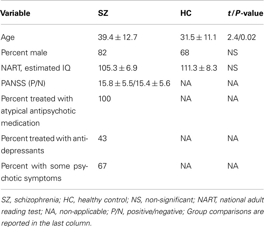
Table 1. Demographic and clinical characteristics of patients with schizophrenia (n = 28) and healthy controls (n = 28).

2.2. ICA Algorithm

The ICA analysis of fMRI data start with the spatial ICA model where X = AS, S = [s₁,…, s _N]^T is an N-by-V source matrix, N is the number of sources, V is the number of voxels and s _i is the ith spatial component. The mixing matrix A is an M-by-N matrix where each column a _i represents the time course for the ith source. The goal of the ICA algorithm is to determine a demixing matrix W such that the sources are estimated using $\widehat{\mathbf{\text{S}}}=\mathbf{\text{WX}}$ under the assumption of statistical independence of spatial components.

The sources of interest in fMRI data are commonly assumed to have a super-Gaussian distribution (Calhoun and Adali, 2006). The standard version of Infomax assuming such distribution sources produces consistent ICs (Correa et al., 2007; Du et al., 2011). It minimizes the mutual information among the estimated sources by maximizing information transfer from the input to the output within a network through a non-linear function (Bell and Sejnowski, 1995). Hence, we apply Infomax in our fMRI analysis. Instead of entering each subject’s data into a separate ICA analysis, we use a group ICA (Calhoun et al., 2001; Erhardt et al., 2011) technique implemented in the Group ICA of fMRI Toolbox (GIFT, 2011) to estimate a set of spatial components.

In the ICA step, ICs belonging to several brain networks are generated. Our classification approach includes the extraction of powerful features from those ICs. The advantage of using ICA is to evaluate the classification power with different networks. Hence, the ICA step is important and necessary in the classification method we presented.

2.3. Classification Preprocessing

The classification procedure uses a leave-one-out method to evaluate performance of the feature extraction framework. For each left-out test subject, the remaining 55 subjects (including controls and patients) comprise the training set. In order to avoid the bias introduced by processing the training and test data together, we perform group ICA each time to decompose the training data. The single-subject spatial maps for the test data are obtained using back-reconstruction via regression, also called spatial-temporal regression (STR; Erhardt et al., 2011).

Group ICA consists of two dimension reduction stages. At the subject level, the number of components for each subject is first reduced to 40 by PCA; the reduced components from each subject are then concatenated. At the group level, the number of components for the aggregate group is reduced to 30. This order has proven to be consistently estimated for fMRI data sets from two AOD sessions and one resting-state session (Li et al., 2011). We then perform ICA on this final set. Since the ICA algorithm is iterative, we use ICASSO (Himberg and Hyvarinen, 2003) in GIFT to improve robustness of the estimated results. ICASSO runs the ICA algorithm several times, producing different estimated components for each run and then collects the components by clustering them based on the absolute value of the correlation between source estimates (Himberg and Hyvarinen, 2003). Reliable estimates correspond to tight clusters including components that have high correlations with each other. We perform ten runs with different initial values on 30 clusters, which latter is the same as the number of estimated components. Instead of using the average of different runs, we select the centrotype of the cluster for each component as the best estimate. Then, for each session of each subject in the training set, spatial components, and time courses are obtained from the back-reconstruction step.

To obtain spatial components for the test subject, we use the ICA model X = AS as the STR model. First, time courses of the test subject are calculated by ${\mathbf{\text{A}}}_t={\mathbf{\text{X}}}_t{\mathbf{\text{S}}}_g^{†},$ where X _t is the observation matrix of the test subject, S _g is the aggregate results estimated from the training group and each column of A _t corresponds to the time course of the test subject. Then spatial components of the test subject are calculated by ${\mathbf{\text{S}}}_t={\mathbf{\text{A}}}_t^{†}{\mathbf{\text{X}}}_t.$ Next, we calculate the mean of spatial components in the training set and convert it to Z-values. The definition of Z-value is Z = (s – μ)/σ, where s is the value of each voxel, μ is the mean of all voxels, and σ is the standard deviation. To generate a mask containing only binary values, we set the values of voxels in the Z-map to be 1 if | Z | > 0.5, otherwise to be 0, then apply this mask to the spatial component obtained from STR to generate a better defined component for later analysis.

The same preprocessing procedure used in the training and test data is then applied to the rest and AOD data set. All spatial components are converted to Z-values. Hence, the image intensities provide a relative strength of the degree to which a particular component contributes to the data, thus enabling us to compare spatial components across different subjects (Calhoun et al., 2001; Allen et al., 2011; Erhardt et al., 2011). Since we have two AOD and one rest data set per subject, we average spatial components of two AOD data sets and convert them to Z-values.

As our data consist of 56 subjects, we perform group ICA 56 times on different training sets and obtain corresponding spatial components of each test subject using STR. However, group ICA introduces a permutation ambiguity. We need to generate several masks to select the same component from each training set. To simplify the problem, we use components obtained from group ICA to generate masks, and then calculate correlations between each spatial component and a particular mask in different training sets. The component providing the largest correlation value corresponds to the same brain region as the mask. Using these procedures, 14 components of interest were selected from 30 ICs based on visual inspection and were correlated with corresponding components in each training set. The 14 components of interest were advanced to the next step.

3. Methods

The feature extraction method for the classification consists of three steps: a two-level feature identification scheme, kernel PCA, and Fisher’s linear discriminant analysis, as illustrated in Figure 1. First, we generate a two-level feature identification scheme to select significant features based on statistical hypothesis testing such as t-tests. Second, we perform KPCA to compute low dimensional representations of the significant features selected in the first step. KPCA computes the higher-order statistics without the combinatorial explosion of time and memory complexity (Schölkopf et al., 1998). Then we apply FLD to further extract features that maximize the ratio of between- and within-class variability.

FIGURE 1

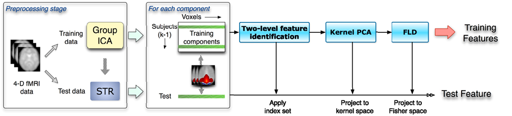
Figure 1. The flow chart shows a leave-one-out scheme given k subjects. This includes the preprocessing stage and the three-phase feature selection and extraction framework. Spatial components as inputs are obtained from the data preprocessing stage. Training and test data are processed separately in the whole procedure.

The kernel Fisher discriminant analysis (KFD) combines the kernel trick with FLD (Mika et al., 1999; Baudat and Anouar, 2000). The KFD always encounters the ill-posed problem in its real-world applications and with KPCA and FLD together, we could make full use of two kinds of methods and achieve a more powerful discriminator (Yang et al., 2005). Our algorithm applies a two-phase KFD using KPCA and FLD together.

3.1. Two-Level Feature Identification

FMRI data are high dimensional in terms of numerous voxels and have high noise levels. Even though we select only a small number of ICs after ICA, each IC still contains more than 60 k voxels, which may provoke over-fitting in a classifier without prior dimension reduction. In order to avoid the “curse of dimensionality” and select significant voxels, we apply one-sample and two-sample t-tests to the selected components.

T-tests are among the most widely used statistical significance measures currently adopted in feature selection. The one-sample t-test is used to infer whether an unknown population mean differs from a hypothesized value. For instance, we have training data x₁,…, x_n assumed to be independent realizations. Then we test the following hypothesis:

$\begin{array}{c}\text{Null}\text{Hypothesis}:H_0:\mu ={\mu }_0\\ \text{Alternate}\text{Hypothesis}:H_1:\mu \ne {\mu }_0.\end{array}$

The mean is estimated by the sample mean $\bar{x}.$ The greater the deviation between $\bar{x}$ and μ₀, the greater the evidence that the hypothesis is untrue. The test statistic t is a function of this deviation, standardized by the standard error of $\bar{x}$. It is defined as

$t=\frac{\bar{x}-{\mu }_0}{\sigma /\sqrt{n}}.$

We compute voxel-wise one-sample t-tests separately for the control and patient groups in the training set, which treats each subject as a random effect and provides a statistical threshold on the components. The null hypothesis is set to be H₀: μ = 0 and the test statistic is treated as the threshold in selecting significant features. The thresholds are the same for both groups and defined as t₁. Voxel positions are recorded in an index set if the t-values are larger than the threshold t₁. Then we obtain a union index set of significantly activated voxels in both control and patient groups.

Next, we compute a voxel-wise two-sample t-test between the two groups, using a two-sample t-test to assess whether the means of the two classes are statistically different from each other by calculating a ratio between the difference of two class means and the variability of the two classes. The training data are selected from two groups, $x_{11},\dots ,x_{1n_1}$ and $x_{21},\dots ,x_{2n_2},$ and it is desired to test the null hypothesis μ₁ = μ₂ (Dalgaard, 2008). The test statistic is defined as

$t=\frac{{\overline{x}}_1-{\overline{x}}_2}{\sqrt{{\sigma }_1^2/n_1+{\sigma }_1^2/n_2}}.$

The threshold of two-sample t-test is denoted as t₂. An index set of significantly different voxels is composed of the voxel positions where two-sample t-statistics are larger than t₂. Next, we calculate the intersection of index sets obtained from one-sample and two-sample t-test to generate a final index set with significant positions in the training set. Then we apply this final index set to components of interest for the test set to select significant voxels. The scheme of the two-level feature identification is shown in Figure 2.

FIGURE 2

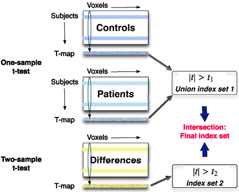
Figure 2. A one-sample t-test is applied across the same components separately to the control and patient groups in the training set. A two-sample t-test is performed to find voxels that are significantly different between two groups. The features including the significantly activated and different voxels are identified in this two-level feature identification scheme.

3.2. Kernel PCA

After the two-level feature identification step, the dimension of features is reduced to thousands (this value depends on t-test thresholds), which, however, is still high to some classifiers. Moreover, in fMRI, activation patterns of BOLD-related sources tend to be spatially smoothed and clustered. These contextual features encoded in the signal sample space are not exploited in a standard ICA framework (Li et al., 2007). Thus, higher-order correlations may exist among voxels. To reduce feature dimensions and take higher-order statistics into account, we apply KPCA to project the input data into a new space using a non-linear mapping and apply linear PCA in this new space.

For a given non-linear mapping Φ, the input data space R ⁿ can be mapped into a new space called feature space F (Schölkopf et al., 1998):

$\begin{array}{c}\text{Φ}:R^n\to F\\ \text{x}=\left(x_1,\dots ,x_n\right)\mapsto \text{Φ}\left(\text{x}\right)=\left({\text{Φ}}_1\left(x\right),\dots ,{\text{Φ}}_N\left(\text{x}\right)\right).\end{array}$

The mapping can lead to a potentially much higher dimensional feature vector in the feature space F. The additional feature dimensions which indicate the complexity of the function class matters can be useful for performing target classification (Müller et al., 2001). KPCA, as described in (Schölkopf et al., 1998; Müller et al., 2001), is shown as follows.

First, given a set of training samples x _k, k = 1,…, M, x _k ∈ R ⁿ, we define an M × M matrix $\widetilde{\mathbf{\text{K}}}$ with entries k(x _i, x _j), where

$k\left({\mathbf{\text{x}}}_i,{\mathbf{\text{x}}}_j\right)=〈\text{Φ}\left({\mathbf{\text{x}}}_i\right),\text{Φ}\left({\mathbf{\text{x}}}_j\right)〉$

is the kernel representation. We obtain centered data Φ(x) by centralizing $\widetilde{\mathbf{\text{K}}}$, such that

$\mathbf{\text{K}}=\widetilde{\mathbf{\text{K}}}-{\mathbf{\text{1}}}_M\widetilde{\mathbf{\text{K}}}-\widetilde{\mathbf{\text{K}}}{\mathbf{\text{1}}}_M+{\mathbf{\text{1}}}_M\widetilde{\mathbf{\text{K}}}{\mathbf{\text{1}}}_M,$

where the matrix 1 _M is the M-by-M matrix with all entries equal to 1/M.

Second, we compute the eigenvectors of K and normalize them in feature space by

${\beta }^j=\frac{1}{\sqrt{{\lambda }_j}}\mathbf{\text{K}}{\alpha }^j,j=1,\dots ,m.$

where m is the dimension after KPCA, λ₁ > λ₂ > … > λ_m denote the m largest positive eigenvalues of the kernel matrix K, α¹,…, α^m are the corresponding eigenvectors, and β¹,…, β^m are the normalized eigenvectors in feature space.

Third, for a training sample x _k, we can obtain the KPCA transformed feature vector y _k = [y_k1, y_k2,…, y_km]^T by y _k = 〈V, Φ(x _k)〉, where V is a matrix of eigenvectors in feature space and specifically,

$y_{kj}=\sum _{l=1}^M{\beta }_l^{j}k\left({\mathbf{\text{x}}}_l,{\mathbf{\text{x}}}_k\right),j=1,\dots ,m.$(1)

For a test data x _i with a mapping Φ(x _i) in feature space, we project the data onto the subspace generated by the training data. Then the KPCA transformed feature vector y _i = [y_i1, y_i2,…, y_im]^T is obtained by (1).

In summary, the following steps are necessary to compute the features for training and test data (Schölkopf et al., 1998): (1) compute the matrix K using all training data, (2) compute its eigenvectors and normalize them in feature space F, and (3) compute projections of training and test data onto the eigenvectors.

Algorithm 1 classifier based on euclidean distance

Require: features of training data and test data as inputs, such that f_i, i = 1, 2, …, 55, and f_t

1. Calculate d_i = ||f_t – f_i||₂, $d^{\left[c\right]}=\frac{1}{n_1}{\Sigma }_{i=1}^{n_1}{d}_i^{\left[c\right]},$ and $d^{\left[p\right]}=\frac{1}{n_2}{\Sigma }_{i=1}^{n_2}{d}_i^{\left[p\right]}$

2. if d^[c] < d^[p]then

3.   the test data belongs to the control group

4. else

5.   the test data belongs to the patient group

6. end if

7. return the class label of the test subject

 Algorithm 2 feature combination algorithm

 Require: for a test subject, input component matrix X _i, i = 1,2, …, m and X _i = (x₁, x₂,…, x₅₆)^T

1. given an initial value num = 0 and calculate the majority value M = m/2 + 1 or M = (m + 1)/2

2. for k = 1 → m do

3.  f _k = $\mathcal{F}$(X _k)

4.  classify the test subject using Algorithm 1

5.  if the test data is classified into the control group then

6.   num ← num + 1

7.  end if

8. end for

9. if num ≥ Mthen

10.  the test data belongs to the control group

11. else

12.  the test data belongs to the patient group

13. end if

14. return the class label of the test subject

3.3. FLD

The Fisher discriminant function aims to achieve an optimal linear dimensionality reduction, by employing a linear projection of the data onto a one-dimensional space, such that an input vector x is projected onto y = w ^Tx , where w is a vector of adjustable weight parameters (Fisher, 1936; Bishop, 1995). In general, the projection onto one dimension leads to a considerable loss of information. However, by adjusting w, we can achieve a projection that maximizes the class separation and also does not lose within-class compactness. The resolution proposed by Fisher is to maximize a function representing the difference between the projected class means, normalized by a measure of the within-class scatter along the direction of w. The Fisher criterion is given by

$J\left(\mathbf{\text{w}}\right)=\frac{{\mathbf{\text{w}}}^T{\mathbf{\text{S}}}_B\mathbf{\text{w}}}{{\mathbf{\text{w}}}^T{\mathbf{\text{S}}}_w\mathbf{\text{w}}},$(2)

where S _B is the between-class covariance matrix and is given by

${\mathbf{\text{S}}}_B=\left({\mathbf{\text{m}}}_2-{\mathbf{\text{m}}}_1\right){\left({\mathbf{\text{m}}}_2-{\mathbf{\text{m}}}_1\right)}^T$

and S _W is the total within-class covariance matrix, given by

$\begin{array}{l}{\text{s}}_w={\displaystyle \sum _{n\in C_1}\left({\text{x}}^n-m_1\right)}{\left({\text{x}}^n-m_1\right)}^T\\ +{\displaystyle \sum _{n\in C_2}\left({\text{x}}^n-m_2\right){\left({\text{x}}^n-m_2\right)}^T.}\end{array}$

The mean vectors of the two groups are given by

${\mathbf{\text{m}}}_1=\frac{1}{n_1}\sum _{n\in C_1}{\mathbf{\text{x}}}^n\text{and}{\mathbf{\text{m}}}_2=\frac{1}{n_2}\sum _{n\in C_2}{\mathbf{\text{x}}}^n,$

where n₁ and n₂ are the numbers of controls and patients in the training set. The objective J(w) is maximized by $\mathbf{\text{w}}\propto {\mathbf{\text{S}}}_W^{-1}\left({\mathbf{\text{m}}}_2-{\mathbf{\text{m}}}_1\right),$ where w is the eigenvector corresponding to the largest eigenvalue of ${\mathbf{\text{S}}}_W^{-1}{\mathbf{\text{S}}}_B.$

3.4. Parameters and Classifier

For different thresholds in the two-level identification scheme, the proposed feature extraction framework generates different features for the training data. In order to obtain a set of features characterized by sufficiently large discrimination power, we select a combination of thresholds t₁ and t₂ that maximizes the value of the objective function J(w) shown in (2) in the training stage. Then the selected thresholds are applied to all data, including training and test data. After obtaining significant features, we calculate the Euclidean distances between the test feature and all training features, such that $d_1^{\left[c\right]},\dots ,d_{n_1}^{\left[c\right]},d_1^{\left[p\right]},\dots ,d_{n_2}^{\left[p\right]},$ where c denotes the healthy control and p the patient group. By comparing the mean distances between the test data and each training group, we classify the test data into the closest group. The classifier algorithm is labeled and described as Algorithm 1.

4. Experimental Results

In our experiments, the AOD and rest data sets are used to evaluate the performance of the proposed feature extraction method. We select 14 components of interest as features to discriminate healthy controls and patients in each data set. The components are labeled as follows and the t-maps for these components are shown in Figure 3: (1) DMN, (2) temporal, (3) motor-temporal, (4) sensorimotor, (5) anterior DMN (medial frontal), (6) anterior frontal, (7) lateral frontal, (8) fronto-insula, (9) motor, (10) posterior parietal, (11) right frontoparietal, (12) left frontoparietal, (13) cerebellum, and (14) medial visual components.

FIGURE 3

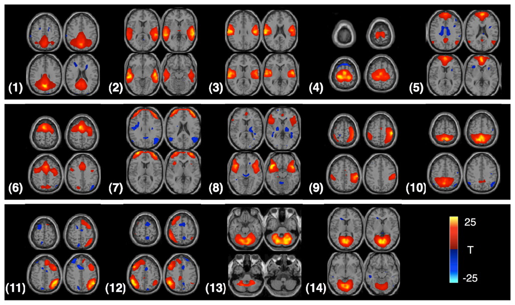
Figure 3. Four slices from each component are shown in the figure; components are identified from the AOD task. Each component is entered into a one-sample t-test and thresholded at P < 1e−7 (corrected for multiple comparisons using the family wise error (FWE) approach, implemented in SPM5).

We first use individual components of interest as inputs of the feature extraction framework. Then a leave-one-out approach is performed to validate the classification procedure. Second, we combine features in a majority vote method to classify the left-out test subject. We show the accuracy, sensitivity, and specificity of the obtained classification results. Accuracy is calculated as the ratio between the number of test data sets classified into the correct group and the total number of test data sets. Sensitivity and specificity are defined and calculated as shown in Table 2.

TABLE 2

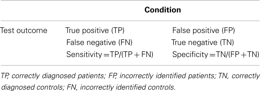
Table 2. The definitions of sensitivity and specificity.

During the training stage, we repeat the process of the two-level feature identification, KPCA and FLD to calculate the value of the objective function in (2) for each combination of thresholds. If the thresholds are selected as large values, a few voxels are retained after the two-level feature identification step. To reduce the computation time and retain more information, we use the values of 0–3 with the increment of 0.5 for t₁ in the one-sample t-test and the same interval for t₂ in the two-sample t-test. We select the combination of thresholds leading to the maximum value of (2) in this range. To implement KPCA, we use the polynomial kernel function primarily due to its simplicity as it has a simpler structure and by selecting different orders, we can control the degree of non-linear mapping. It is defined as

$k\left(\mathbf{\text{x,y}}\right)={\left({\mathbf{\text{x}}}^T\mathbf{\text{y}}+1\right)}^d,$

where d is the order of the polynomial kernel. Also, our experimental results show that the polynomial kernel function performs better than the Gaussian kernel in KPCA in our task when tested with a number of kernel widths. For the polynomial kernel, we use d = 3 in our experiments. The dimensionality of the underlying KPCA space cannot be allowed to exceed M – c, where M is the total number of training samples available and c is the number of classes (Martínez and Kak, 2001). In our study, M = 55, c = 2. Thus, we set the dimension of principal components after KPCA to 53. Figure 4 shows visualization of features for controls versus patients after each feature extraction step. Results show that training samples are linearly separable after the three-phase feature extraction.

FIGURE 4

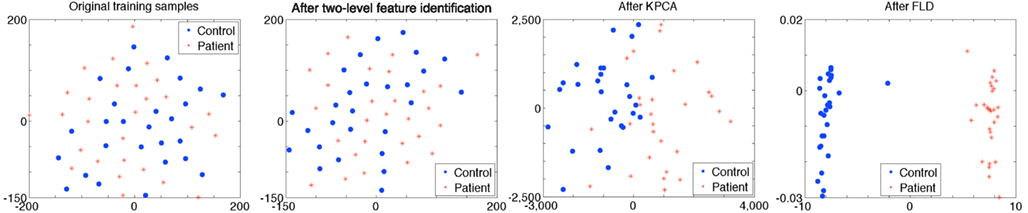
Figure 4. The figure shows features for controls versus patients after each feature extraction step. Each dot represents an individual and the color of the dot indicates the correct diagnosis of either control (blue) or schizophrenia (red). Individuals are close to each other if the Euclidean distances between training data are small. The original training samples cannot be separated by a linear classifier. A two-level feature identification step is used to select significantly different voxels. After KPCA, most of training samples separate to two groups. Training samples are linearly separable and a maximum margin is obtained after FLD. Parameters in two-level feature identification step are t₁ = 0.5 and t₂ = 0.5, which are selected during the training stage using the DMN component (from rest data) as input to the framework.

4.1. Classification Using AOD Data

4.1.1. Classification using individual component

Components selected from ICA results are independent brain images, each of which can be considered as an independent feature vector and used as the input of our feature extraction framework. We find 14 components of interest in our AOD data. As shown in Figure 1, after the training stage, a significant feature is extracted from one component for each subject. Then we use a simple classifier given in Algorithm 1 to discriminate the test data. Classification results are shown in Table 3.

TABLE 3

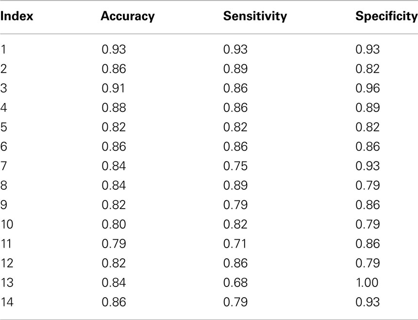
Table 3. Classification results with AOD data (one component as features).

4.1.2. Classification using combined features

Since each component of interest may provide different information in discriminating healthy controls and patients, we also wanted to evaluate results when incorporating more than one component. We select m components from the 14 components of interest and input them into $\mathcal{F}$, denoting the feature extraction framework shown in Figure 1. Then for each test subject, we use classification results obtained from m components to provide a vote and classify the test subject into the group based on the majority vote. If more than half of selected components classify the test data into the control group, then the test subject is assigned to the control group, otherwise the test subject is assigned to the patient group. The algorithm for combining features is labeled and described as Algorithm 2. In our experiments, we explore all possible combinations of the 14 components of interest to discriminate the test data. The component combinations leading to the highest accuracy is shown in Table 5.

4.2. Classification Using Rest Data

4.2.1. Classification using individual component

In the rest data, we select components of interest as same as those in AOD data. We select 13 components of interest from ICA results, corresponding to those obtained above, with the exception of the motor-temporal component. This latter component could be estimated in the control group, but it could not be consistently derived from the patient group. Thus, we exclude the motor-temporal component in the classification of rest data. We extract features using the proposed framework from these 13 ICs and classify the test data; results are shown in Table 4.

TABLE 4

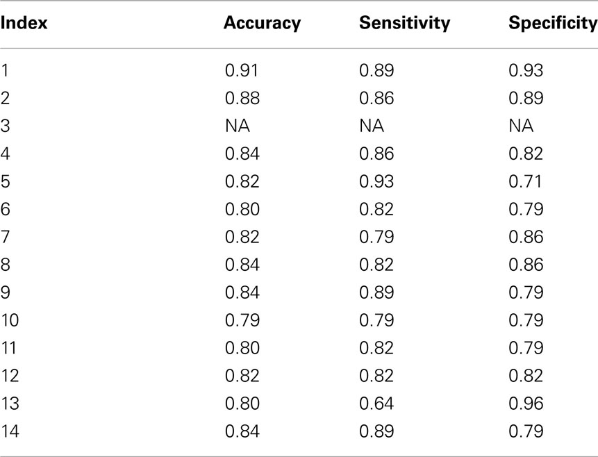
Table 4. Classification results with rest data (one component as features).

4.2.2. Classification using combined features

The feature combination method in Algorithm 2 is used in the rest data set. Since the motor-temporal component is not included in the experiment, the component with index 3 is not used in the feature combination. We assess every combination of the 13 components to discriminate the test data and then evaluate classification performance. Several combinations lead to similar classification results; some of those with the highest accuracy are shown in Table 5.

TABLE 5

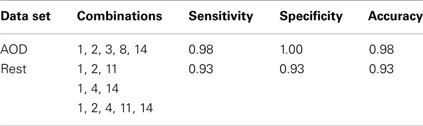
Table 5. Classification results using feature combination.

5. Discussion

5.1. During AOD Task and at Rest

In this paper, we propose a novel method for effective feature selection and extraction. We evaluate the performance of several components of interest extracted as features using our method by discriminating healthy controls from schizophrenia patients during an AOD task and at rest. Our results show that features extracted from the DMN and the motor-temporal component lead to significantly high classification accuracy, providing additional support to previous studies, which noted the importance of these components for discriminating patients with various mental diseases from controls (Calhoun et al., 2008b; Sui et al., 2009). We also find that components leading to the highest classification accuracy, including DMN, temporal, and medial visual regions, are consistently included among the combined components for both data sets, since similar components have been observed for participants during an AOD task and at rest (Calhoun et al., 2008a). Overall, the AOD task appears to be more discriminating across more components than the resting fMRI data as shown in Figure 5.

FIGURE 5

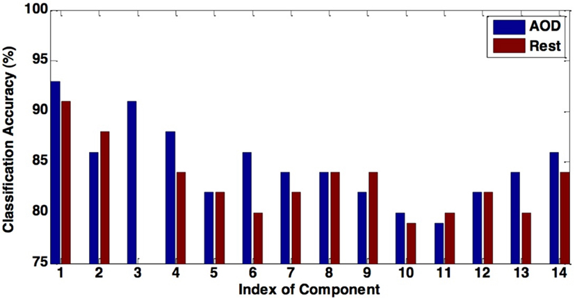
Figure 5. The figure shows the comparison between the classification accuracy in AOD and rest data. Using most of components of interest can lead to a higher accuracy in the AOD data than the rest data.

The DMN is one of the most widely analyzed networks derived from resting-state fMRI data. It is commonly observed to deactivate during task-based fMRI experiments proportionately to task difficulty (McKiernan et al., 2003). This network shows significant activity differences between controls and schizophrenia patients (Garrity et al., 2007), although in most such comparisons, including the current analysis, patients are taking antipsychotic medications, which themselves affect DMN activity (Lui et al., 2010) and may thus exaggerate patient/control differences. In our classification results shown in Tables 3 and 4, the discrimination accuracy is highest using features extracted from DMN for both data sets. Moreover, classification accuracy is slightly higher for AOD than rest data. In DMN, activity decreases are consistent across a wide variety of task conditions (Raichle and Snyder, 2007; Raichle, 2010). Consequently, there are more patient/control DMN differences during the AOD task than at rest.

Other regions important for diagnostic discrimination include temporal and motor areas. The temporal region is involved in auditory processing and motor areas are responsible for the perception and execution of actions. Since participants were asked to press a button when they heard the target sound in the AOD task, brain regions related to auditory and motor functions are expected to be highly activated. Two components related to auditory function are derived from AOD data, one designated the temporal and the other the motor-temporal component. Researchers in several fields postulate important links between auditory and motor areas (Hickok et al., 2003). In our results, using the motor-temporal component as a classification feature reveals a high accuracy in discriminating controls and patients in the AOD task. Conversely, in the rest data, the motor-temporal component could not be consistently estimated in patients but was obvious in the control group. The temporal and motor-temporal components are clearly separated in the control group at rest but not so in patients. This is shown in Figure 6. This suggests that the auditory-motor link is weaker in schizophrenia than in healthy controls. The motor-temporal component can be directly estimated in the patient group during the AOD task, since participants are instructed to press a button when they hear the target sound; this condition forces the motor-temporal component to be estimated. Our numerical results in Table 4 show that using the temporal component as a feature leads to a higher accuracy for rest compared to AOD data. Since patients may lose attention and/or perform poorly during a task, using other motor-related components (such as sensorimotor, anterior frontal, and cerebellum) in AOD data also lead to a high accuracy in our results.

FIGURE 6

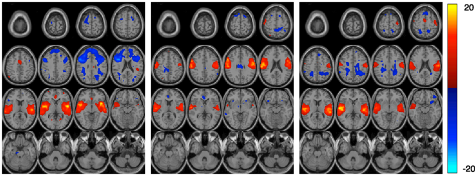
Figure 6. The figure shows three estimated components in the rest data set. Each component is entered into a one-sample t-test and thresholded at P < 0.01 (corrected for multiple comparisons using FWE) shown with 16 slices. The left and middle components are the estimated temporal and motor-temporal components in the control group, respectively. The right component is the only temporal related component estimated in patients.

The feature combination data reveal that a combination of DMN, temporal, motor-temporal, fronto-insula, and medial visual components results in the highest classification accuracy for AOD data. These five components are task-negative networks. In the rest data, several combinations of components result in the highest accuracy. These components, including DMN, temporal, and medial visual regions, are consistently included among those combined components for both data sets. The fronto-insula component is often recruited by cognitively demanding tasks and frequently interpreted as a part of a task-related activation network (Seeley et al., 2007). Thus, the fronto-insula component might be expected to have more significant effect in discriminating groups in AOD data, derived from performance of an actual task, than in rest data.

5.2. Motion Artifacts

Motion artifacts are common causes of image degradation in fMRI, and patients are more prone to exhibit body movements during scanning procedures for a variety of reasons. Hence, motion artifacts may amplify differences between controls and patients in classification results. Our fMRI data are preprocessed in SPM (Friston et al., 1995; SPM5, 2011) to minimize movement artifacts. In the preprocessing procedure, a set of realignment parameters reflecting the relative orientations of the data is saved for each subject. To evaluate the influence of motion artifacts in our classification results, we then use these realignment parameters as features to perform another classification.

In processing the AOD data set, we average realignment parameters from the two sessions per participant resulting in a 249 × 6 matrix for each subject (249 time points, each of which has 6 parameters). Similarly, in the rest data set, a 204 × 6 matrix is obtained for each subject (from 204 time points in these data). We use a leave-one-out cross-validation and the same classifier in Algorithm 1 to evaluate the classification results. To certify the result, we extract several kinds of features from the realignment parameters to perform the same classification. For each subject, the feature vector comprises the mean value of parameters of each time point. Another approach is to use feature vectors consisting of the maximum value of parameters of each time point, or the feature vector comprises mean (or maximum) values across all time points. In addition, we can select mean (or maximum) values of the parameter matrix for each subject as the feature. For the AOD data, the accuracy of using realignment parameters as features is from 48 to 54% and for the rest data, the accuracy is from 34 to 52%. Therefore, motion artifacts appear to have little impact on our classification results.

5.3. Multiple Sessions in AOD Data

Our analysis used two runs of AOD task data and one session of rest data. For a representative comparison, we also use the first session of AOD data in the same analysis. The results are almost the same as previous and remain the same when we combine features in a majority vote method. The most likely reason for these results is that we treat two sessions of data as two different subjects in the group ICA analysis, first doubling the number of subjects in AOD data. We then average the components from the two sessions as the input of our classification framework. This procedure has few effects on our classification results.

5.4. Avoid “Double Dipping” in the Analysis

Double dipping, the use of the same data set for selection and selective analysis, provides distorted descriptive statistics and invalid statistical inference whenever the resulting statistics are not inherently independent of the selection criteria under the null hypothesis (Kriegeskorte et al., 2009). In our classification, including the step that ICs of training data are selected by group ICA and ICs of the left-out test data are generated by spatial-temporal regression, initially separates the training and test data. Then, we use only training data to select thresholds in the two-level feature identification scheme and generate feature spaces in Kernel PCA and Fisher’s linear discriminant analysis. The left-out test feature is obtained by applying selected thresholds to ICs and projecting selected voxels to the training feature space. For different training sets and corresponding left-out test subjects, the classification procedures are independent. Thus, the problem of using the same data set both to train and to test classification is completely avoided in our method.

5.5. Validation of Three-Phase Feature Extraction

In order to see whether all three steps were essential, we eliminated the first step and performed KPCA and FLD directly on all voxels. This two-step approach resulted in significant performance loss. For example, features extracted from DMN component, without the first step, lead to a classification accuracy of 73%, which is significantly lower than the current result shown in Section 4. Those unselected voxels in the first step are more likely to be noise and do not provide sufficient information to discriminate patients from healthy controls. Hence, the three-phase feature extraction framework is meaningful and necessary in the classification method we have presented.

6. Conclusion

We introduce a three-phase feature extraction framework that takes higher-order statistics into account and satisfies the Fisher’s criterion, with components of interest estimated from ICA algorithm as inputs. Three steps of the framework include a two-level feature identification scheme, KPCA, and FLD. First, a two-level feature identification scheme is performed to select significantly activated and discriminative voxels from components of interest. Second, KPCA is used to extract non-linear features from the selected significant voxels by taking into account higher-order statistics. Then, FLD is performed to further extract features that maximize the ratio of between- and within-class variability. Experimental results using both AOD and rest data are included to demonstrate the performance of the proposed framework. Results show that features extracted from DMN and motor-temporal components lead to significantly high classification accuracies. Moreover, we implement a majority vote method to incorporate different components of interest into combined features. Several components, including DMN, temporal, and medial visual regions, are consistently contained in the combined components leading to the best classification accuracy for both data sets. By comparing the classification results from AOD and rest data, we find significant interactions and differences between these data sets for several components of interest. One possible limitation of the present work is that all patients were on psychotropic medication during the testing. It is possible that the medication effects could artificially enhance our classification results. However, the obtained high classification accuracy, combined with the fact that several networks all have powerful ability to distinguish patients from controls, suggests that this is not a dominant effect. Another possible limitation is the small number of subjects used in the current study. Hence, it is desirable to determine to what degree the medication impacts functional classification and it is desirable to extend the database to include more subjects. However, features extracted using the method we presented show very promising results in terms of classification performance and it is reasonable to say that the framework can be applied to extract significant features from components of interest that can be used to discriminate patients from healthy controls.

Conflict of Interest Statement

The authors declare that the research was conducted in the absence of any commercial or financial relationships that could be construed as a potential conflict of interest.

References

Allen, E. A., Erhardt, E. B., Wei, Y., Eichele, T., and Calhoun, V. D. (2011). Capturing inter-subject variability with group independent component analysis of fMRI data: a simulation study. Neuroimage 59, 4141–4159.

Pubmed Abstract | Pubmed Full Text | CrossRef Full Text

Arribas, J. I., Calhoun, V. D., and Adali, T. (2010). Automatic bayesian classification of healthy controls, bipolar disorder, and schizophrenia using intrinsic connectivity maps from fMRI data. IEEE Trans. Biomed. Eng. 57, 2850–2860.

Pubmed Abstract | Pubmed Full Text | CrossRef Full Text

Baudat, G., and Anouar, F. (2000). Generalized discriminant analysis using a kernel approach. Neural Comput. 12, 2385–2404.

Pubmed Abstract | Pubmed Full Text | CrossRef Full Text

Bell, A. J., and Sejnowski, T. J. (1995). An information-maximization approach to blind separation and blind deconvolution. Neural Comput. 7, 1129–1159.

Pubmed Abstract | Pubmed Full Text | CrossRef Full Text

Bishop, C. M. (1995). Neual Neworks for Pattern Recognition. New York, NY: Oxford University Press.

Calhoun, V. D., and Adali, T. (2006). Unmixing fMRI with independent component analysis. IEEE Eng. Med. Biol. Mag. 25, 79–90.

Pubmed Abstract | Pubmed Full Text | CrossRef Full Text

Calhoun, V. D., Adali, T., Pearlson, G. D., and Pekar, J. J. (2001). A method for making group inferences from functional MRI data using independent component analysis. Hum. Brain Mapp. 14, 140–151.

Pubmed Abstract | Pubmed Full Text | CrossRef Full Text

Calhoun, V. D., Kiehl, K. A., and Pearlson, G. D. (2008a). Modulation of temporally coherent brain networks estimated using ICA at rest and during cognitive tasks. Hum. Brain Mapp. 29, 828–838.

CrossRef Full Text

Calhoun, V. D., Maciejewski, P. K., Pearlson, G. D., and Kiehl, K. A. (2008b). Temporal lobe and default hemodynamic brain modes discriminate between schizophrenia and bipolar disorder. Hum. Brain Mapp. 29, 1265–1275.

CrossRef Full Text

Correa, N., Adali, T., and Calhoun, V. D. (2007). Performance of blind source separation algorithms for fMRI analysis using a group ICA method. Magn. Reson. Imaging 25, 684–694.

Pubmed Abstract | Pubmed Full Text | CrossRef Full Text

Dalgaard, P. (2008). Introductory Statistics with R. New York, NY: Springer.

Demirci, O., Clark, V. P., Magnotta, V. A., Andreasen, N. C., Lauriello, J., Kiehl, K. A., Pearlson, G. D., and Calhoun, V. D. (2008). A review of challenges in the use of fMRI for disease classification/characterization and a projection pursuit application from a multi-site fMRI schizophrenia study. Brain Imaging Behav. 2, 207–226.

CrossRef Full Text

Du, W., Li, H., Li, X.-L., Calhoun, V. D., and Adali, T. (2011). “ICA of fMRI data: performance of three ICA algorithms and the importance of taking correlation information into account,” in Proceedings of the 8th IEEE International Symposium on Biomedical Imaging, Chicago, 1573–1576.

Pubmed Abstract | Pubmed Full Text

Erhardt, E. B., Rachakonda, S., Bedrick, E. J., Allen, E. A., Adali, T., and Calhoun, V. D. (2011). Comparison of multi-subject ICA methods for analysis of fMRI data. Hum. Brain Mapp. 12, 2075–2095.

CrossRef Full Text

Fisher, R. (1936). The use of multiple measures in taxonomic problems. Ann. Eugen. 7, 179–188.

CrossRef Full Text

Ford, J. (1999). Schizophrenia: the broken p300 and beyond. Psychophysiology 36, 667–682.

Pubmed Abstract | Pubmed Full Text | CrossRef Full Text

Ford, J., Shen, L., Makedon, F., Flashman, L. A., and Saykin, A. J. (2002). “A combined structural-functional classification of schizophrenia using hippocampal volume plus fMRI activation,” in Second Joint EMBS/BMES Conference, Houston, 48–49.

Friston, K. J., Frith, C. D., Frackowiak, R. S., and Turner, R. (1995). Characterizing dynamic brain responses with fMRI: a multivariate approach. Neuroimage 2, 166–172.

Pubmed Abstract | Pubmed Full Text | CrossRef Full Text

Garrity, A. G., Pearlson, G. D., McKiernan, K., Lloyd, D., Kiehl, K. A., and Calhoun, V. D. (2007). Aberrant òdefault modeó functional connectivity in schizophrenia. Am. J. Psychiatry 164, 450–457.

Pubmed Abstract | Pubmed Full Text | CrossRef Full Text

GIFT. (2011). Group ICA of fMRI Toolbox (GIFT). Available at: http://mialab.mrn.org/software/gift/index.html

Hickok, G., Buchsbaum, B., Humphries, C., and Muftuler, T. (2003). Auditory-motor interaction revealed by fMRI: speech, music, and working memory in area Spt. J. Cogn. Neurosci. 15, 673–682.

Pubmed Abstract | Pubmed Full Text | CrossRef Full Text

Himberg, J., and Hyvarinen, A. (2003). “ICASSO: software for investigating the reliability of ICA estimates by clustering and visualization,” in IEEE Workshop on Neural Network Signal Processing, Toulouse, 259–268.

Hotelling, H. (1933). Analysis of a complex of statistical variables into principal components. J. Educ. Psychol. 24, 417–441.

CrossRef Full Text

Kiehl, K. A., Stevens, M. C., Laurens, K. R., Pearlson, G., Calhoun, V. D., and Liddle, P. F. (2005). An adaptive reflexive processing model of neurocognitive function: supporting evidence from a large scale (n=100) fMRI study of an auditory oddball task. Neuroimage 25, 899–915.

Pubmed Abstract | Pubmed Full Text | CrossRef Full Text

Kriegeskorte, N., Simmons, W. K., Bellgowan, P. S. F., and Baker, C. I. (2009). Circular analysis in systems neuroscience: the dangers of double dipping. Nat. Neurosci. 12, 535–540.

Pubmed Abstract | Pubmed Full Text | CrossRef Full Text

Levin, J. M., Ross, M. H., and Renshaw, P. F. (1995). Clinical applications of functional MRI in neuropsychiatry. J. Neuropsychiatry Clin. Neurosci. 7, 511–522.

Pubmed Abstract | Pubmed Full Text

Li, X.-L., Ma, S., Calhoun, V. D., and Adali, T. (2011). “Order detection for fMRI analysis: joint estimation of downsampling depth and order by information-theoretic criteria,” in Proceedings of the 8th IEEE International Symposium on Biomedical Imaging, Chicago, 1945–7928.

Pubmed Abstract | Pubmed Full Text

Li, Y.-O., Adali, T., and Calhoun, V. D. (2007). A feature-selective independent component analysis method for functional MRI. Int. J. Biomed. Imaging 2007, 12.

CrossRef Full Text

Lui, S., Li, T., Deng, W., Jiang, L., Wu, Q., Tang, H., Yue, Q., Huang, X., Chan, R. C., Collier, D. A., Meda, S. A., Pearlson, G., Mechelli, A., Sweeney, J. A., and Gong, Q. (2010). Short-term effects of antipsychotic treatment on cerebral function in drug-naive first-episode schizophrenia revealed by resting state functional magnetic resonance imaging. Arch. Gen. Psychiatry 67, 783–792.

Pubmed Abstract | Pubmed Full Text | CrossRef Full Text

Martínez, A. M., and Kak, A. C. (2001). PCA versus LDA. IEEE Trans. Pattern Anal. Mach. Intell. 23, 228–233.

CrossRef Full Text

McCarley, R. W., Faux, S. F., Shenton, M. E., Nestor, P. G., and Adams, J. (1991). Event-related potentials in schizophrenia: their biological and clinical correlates and a new model of schizophrenic pathophysiology. Schizophr. Res. 4, 209–231.

Pubmed Abstract | Pubmed Full Text | CrossRef Full Text

McKeown, M. J., Makeig, S., Brown, G. G., Jung, T. P., Kindermann, S. S., Bell, A. J., and Sejnowski, T. J. (1998). Analysis of fMRI data by blind separation into independent spatial components. Hum. Brain Mapp. 6, 160–188.

Pubmed Abstract | Pubmed Full Text | CrossRef Full Text

McKiernan, K. A., Kaufman, J. N., Kucera-Thompson, J., and Binder, J. R. (2003). A parametric manipulation of factors affecting task-induced deactivation in functional neuroimaging. J. Cogn. Neurosci. 15, 394–408.

Pubmed Abstract | Pubmed Full Text | CrossRef Full Text

Mika, S., Rätsch, G., Weston, J., Schölkopf, B., and Müller, K. R. (1999). Fisher discriminant analysis with kernels. IEEE Workshop Neural Netw. Signal Process. 9, 41–48.

Müller, K. R., Mika, S., Rätsch, G., Tsuda, K., and Schölkopf, B. (2001). An introduction to kernel-based learning algorithms. IEEE Trans. Neural Netw. 12, 181–201.

Pubmed Abstract | Pubmed Full Text | CrossRef Full Text

Pearson, K. (1901). On lines and planes of closest fit to systems of points in space. Philos. Mag. 2, 559–572.

Raichle, M. E. (2010). Two views of brain function. Trends Cogn. Sci. (Regul. Ed.) 14, 180–190.

Pubmed Abstract | Pubmed Full Text | CrossRef Full Text

Raichle, M. E., and Snyder, A. Z. (2007). A default mode of brain function: a brief history of an evolving idea. Neuroimage 37, 1083–1090; discussion 1097–1099.

Pubmed Abstract | Pubmed Full Text | CrossRef Full Text

Schölkopf, B., Smola, A., and Müller, K.-R. (1998). Nonlinear component analysis as a kernel eigenvalue problem. Neural Comput. 10, 1299–1319.

CrossRef Full Text

Seeley, W. W., Menon, V., Schatzberg, A. F., Keller, J., Glover, G. H., Kenna, H., Reiss, A. L., and Greicius, M. D. (2007). Dissociable intrinsic connectivity networks for salience processing and executive control. J. Neurosci. 27, 2349–2356.

Pubmed Abstract | Pubmed Full Text | CrossRef Full Text

Shinkareva, S. V., Ombao, H. C., Sutton, B. P., Mohanty, A., and Miller, G. A. (2006). Classification of functional brain images with a spatio-temporal dissimilarity map. Neuroimage 33, 63–71.

Pubmed Abstract | Pubmed Full Text | CrossRef Full Text

SPM5. (2011). Statistical Parametric Mapping. Available at: http://www.fil.ion.ucl.ac.uk/spm/software/spm5

Sui, J., Adali, T., Pearlson, G. D., and Calhoun, V. D. (2009). An ICA-based method for the identification of optimal fMRI features and components using combined group-discriminative techniques. Neuroimage 46, 73–86.

Pubmed Abstract | Pubmed Full Text | CrossRef Full Text

Yang, J., Frangi, A. F., Yang, J.-Y., Zhang, D., and Jin, Z. (2005). KPCA plus LDA: a complete kernel Fisher discriminant framework for feature extraction and recognition. IEEE Trans. Pattern Anal. Mach. Intell. 27, 230–244.

Pubmed Abstract | Pubmed Full Text | CrossRef Full Text