MEG and fMRI fusion for non-linear estimation of neural and BOLD signal changes

Introduction

Magnetoencephalography (MEG) and functional magnetic resonance imaging (fMRI) both provide indirect views of the underlying neural activity. Focusing our attention on cortical regions of the brain, we can assume that the common source of the signal for both modalities is local and incoming synaptic activity as is currently understood (Logothetis and Wandell, 2004). Nevertheless, the physical mechanisms of signal generation are quite different and lead to substantial differences in signal properties (Hämäläinen et al., 1993; Huettel et al., 2004).

Due to a high effective temporal sampling rate, on the order of milliseconds, MEG can provide instantaneous measurements of large-scale synchronous electromagnetic phenomena introduced by neural activity. On the other hand, the neurovascular transformation of neural activity into the fMRI signal can be measured with full brain coverage with high spatial resolution without a spatial inverse problem. The two modalities have complementary strengths and weaknesses. For example, the ill-posed inverse problem accompanying neural activity (Sekihara et al., 2001; Halchenko et al., 2005; Jun et al., 2005). MEG analysis becomes an issue when the goal is localization of the The localized spatial resolution of fMRI allows one to concentrate on the relationship among brain regions. In this case, the dynamical properties of a modality gain high importance. However, fMRI is unable to reflect neural activity dynamics with the temporal resolution and quality found in MEG. Furthermore, studying the temporal properties of neuronal causes via fMRI is hampered by the complexity of the blood oxygenation level dependent (BOLD) signal generation from the underlying neural activity. Analyzing fMRI and MEG simultaneously allows us to focus on statistical properties of brain activity and neural activity in particular and overcome limitations accompanying each of these modalities.

In this paper, we present a Bayesian framework for information fusion of fMRI and MEG data. Our framework ties these two modalities together through a hidden (latent) state variable that represents neural activity. Thus, our model provides a high-resolution statistical estimate of neural activity that takes advantage of the different strengths of fMRI and MEG data. Many existing approaches to data fusion in functional neuroimaging (Dale et al., 2000; Daunizeau et al., 2007; Jun et al., 2008) are driven by desire to alleviate the spatial inverse problem of bioelectric modalities. In analysis of fMRI data temporal inverse problem becomes important when hemodynamic parameters are unknown (Riera et al., 2004). This paper focuses mainly on the temporal aspects and emphasizes the temporal inverse problem. Further, we show that the combined analysis stabilizes the solution of the fMRI forward problem, delivers a better estimate (in the mean squared error (MSE) sense) of the neural activity than either of the modalities alone, and improves the computational efficiency of estimation of probability distributions of unobserved neural activity.

Although neural activity estimation from the BOLD response can be accomplished using deterministic methods (Vakorin et al., 2007), several studies demonstrate advantages of applying probabilistic approaches to this problem (Friston et al., 2003; Riera et al., 2004; Johnston et al., 2008; Murray and Storkey, 2008). Bayesian methods are essentially data driven (e.g., in the case of non-informative priors) and this ability to use available data sources is very important in practice. For example, in the Bayesian framework information fusion of electroencephalography (EEG) and fMRI has been performed using a variational Bayesian analysis by Daunizeau et al. (2007) and in a Markov chain Monte Carlo (MCMC) setting where fMRI was used as a prior to MEG analysis by Jun et al. (2008). In the analysis of MEG, the probabilistic Bayesian approach was successively demonstrated by Schmidt et al. (1999) and then subsequently developed in other works (Bertrand et al., 2001; Jun et al., 2005). In Bayesian and, in general, probabilistic approaches the system is modeled with the joint probability distribution over random variables, which represent different aspects of the system. Quantities of interest and their distributions are discovered from the available information through systematic application of probability calculus (Gelman et al., 2003). Probabilistic Bayesian approaches are attractive in their inherent ability of providing confidence estimates automatically, since the result is usually not a single solution but rather a distribution of likely solutions (Gelman et al., 2003). An additional and important benefit of these methods is their relatively easy extensibility to different numbers of data sources and flexible incorporation of prior information. Other relevant data-driven approaches to multimodal data analysis include canonical correlation analysis (CCA; Bießmann et al., 2010) as well as other approaches (Eichele et al., 2005, 2008; Moosmann et al., 2008).

In this work, we formulate the problem of information fusion as a general model of latent variable modeling in the context of dynamic Bayesian networks (DBNs; Murphy, 2002), and demonstrate integrated analysis of fMRI and MEG using a sequential Monte Carlo method of particle filtering (Doucet et al., 2001). While the DBN framework is quite general and potentially adaptable to many neuroimaging inference problems, in this paper we focus on a special case. Specifically, we demonstrate the approach on a single activity source. Although it is based on the assumption that a single source suffices in describing observations, we show results on simulated and real data that serve as a proof of concept and are encouraging by themselves. Our results demonstrate the plausibility of the approach for functional data analysis and encourage a subsequent extension to more complex and physiologically plausible models.

Information in the data enters the DBN formulation through likelihood functions. In order to construct these for fMRI and MEG we need to use forward models that produce reliable estimates for BOLD response and magnetic measurements. Mechanisms of BOLD signal generation as a result of neural activity are currently not fully understood (Logothetis and Wandell, 2004; Raichle and Mintun, 2006). However, sufficient progress has been made with the Balloon model of Buxton et al. (1998), where the dynamics of venous volume have been connected to the BOLD response. Changes in cerebral blood flow, venous volume and total deoxyhemoglobin are treated as non-linear functions of physiological parameters and neuronal activity. The model was updated by Friston et al. (2000) with an additional system connecting neuronal activity changes to changes in blood flow (through the flow inducing signal) and subsequently changes in venous volume. Although the input to the system was treated as stimulus sequence by Friston et al. (2000), it has been interpreted and used by others as neural activity (Riera et al., 2004; Vakorin et al., 2007). This hemodynamic forward model (HFM) provides a tool for the study of the dynamics of fMRI as an effect of neuronal generation. In contrast to the HFM, the MEG forward model is linear for a source with fixed known locations and has high temporal resolution. If we think of neural activity as the electric activity, then we can compute its instantaneous effect on the gradiometer measurement. The model is well studied and understood (Hämäläinen et al., 1993).

Some research does not exploit the connection provided by the HFM, treating the input to the model as stimulus time course, rather than neuronal activity (Friston et al., 2003; Stephan et al., 2007; Johnston et al., 2008). When, however, the connection is exploited it is possible to estimate the unobserved neural activity, such as local field potential (Mukamel et al., 2005), according to the HFM. This estimation can be performed by formulating the problem as a state space model by Riera et al. (2004) or as a non-linear optimization problem by Vakorin et al. (2007). We adopt the HFM as the forward model of BOLD signal generation from the underlying neural activity. We also treat the neural activity as electric activity and properly scale it to make it suitable for input to MEG and HFM forward models.

In this study, we use continuous data for both fMRI and MEG modalities (the observed state) and brain activity (the hidden state). This is in contrast to the methods that quantize the data and treat it is as values of discrete random variables (Burge et al., 2007; Rajapakse and Zhou, 2007). We perform neural activity estimation from fMRI-only, MEG-only and the combined measurements. We compare the results based on the ability to estimate neural activity and track the BOLD response. Comparison with known ground truth of a synthetic dataset allows us to (a) reveal exact patterns of the effect of the fusion, (b) vary such parameters as signal-to-noise ratio (SNR) and trace their influence on the analysis. In addition, we perform the analysis on an experimental fMRI and MEG dataset, where both modalities are collected from the same subject in two separate runs using the same visual event-related paradigm.

Dynamic Model

If hidden neural activity is represented by a random variable, then several classical approaches can be used to infer the values of this variable through observations. For the case of a discrete hidden random variable and discrete observations the hidden Markov model (HMM) remains the model of choice (Rabiner, 1989). Discrete random variables have problems when the underlying phenomena are continuous and quantization that would preserve maximal information is very hard. In this case one can use the Kalman filter and its numerous modifications (Murphy, 2002). All these and even more complicated models are generalized by DBNs (Murphy, 2002).

A DBN can consist of random variables with different types: discrete random variables (multinomial probability mass functions (PMF)), Gaussian random variables, arbitrary distributions of continuous random variables and other variants (discrete, continuous, and hybrid). The most general and the hardest case for inference of the hidden variables is the case of continuous variables of various densities.

We want to demonstrate benefits of combined analysis of fMRI and MEG measurements. In order to produce clear and directly interpretable results, in this study we concentrate on a case with a single hidden variable. Of major importance in this paper is the task of inferring the values of this variable conditioned on the MEG and fMRI observations. Figure 1 displays an example region of interest (ROI) in the bank of the superior temporal sulcus of the left hemisphere, whose activity needs to be inferred.

FIGURE 1

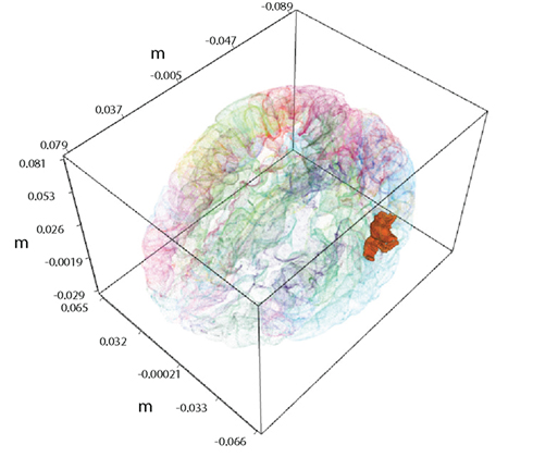
Figure 1. A single active ROI in the brain, shown with the solid color. It is the left hemisphere the bank of the superior temporal sulcus from the FreeSurfer atlas.

The graphical structure of the DBN used in this paper is shown in Figure 2.

FIGURE 2

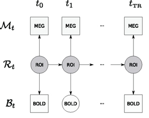
Figure 2. Graphical structure of the DBN that is used in this paper – displayed is a window for a single TR. Observations are denoted by squares (MEG and BOLD); hidden variables are denoted by circles (neural activity in an ROI and unobserved BOLD time points); arrows denote transition and observation models. Due to the sampling frequency difference, many MEG observations are available per single fMRI TR. Time between t_i and t_i+1 corresponds to the MEG sampling time period.

Let us denote the random variable for the ROI with ℛ, for the BOLD response with ℬ and for MEG measurements with 𝒩. We consider separate analysis when measurements from only a single modality are available, as well as a joint analysis, when both data sources are available but not necessary simultaneously. MEG random variable ℳ is a vector random variable containing readings from all MEG sensors. Subscript denotes the time point at which the random variable is considered. In order to denote a sequence of natural numbers we use the column notation: a sequence from 0 to N with step size 1 is denoted by 0:N. The probabilistic model associated with the graphical structure of Figure 2 can be described with the following joint distribution:

The graph from Figure 2 encodes assumptions of the model. The Markov assumption amounts to P(ℛ_t+1|ℛ_0:t) = P(ℛ_t+1|ℛ_t). The stationarity assumption leads to parameter tying of the DBN and fixes the transition P(ℛ_t+1|ℛ_t) and observation models P(ℳ_t|ℛ_t) and P(ℬ_t|⊥ℛ_t) across time steps. We need to define the transition and observation models to complete the description.

In this paper we settle on relatively simple but powerful models suitable to the problem we are working with:

• The linear Gaussian transition model from ℛ_t to ℛ_t+1:

where η_t is zero-mean, unit-variance Gaussian noise, and k and σℛ are estimated from the data. The model corresponds to the following conditional probability density:

• The BOLD response observation model:

where HFM denotes hemodynamic forward model (Hemodynamic Model) and is the variance parameter for fMRI observations, and η_t is Gaussian as before. The resulting conditional probability density is:

where fMRI_t is the measurement at time t.

• MEG observation model:

where MFM denotes MEG forward model, is the variance parameter for MEG observations, and η_t is Gaussian as before. The resulting conditional probability density is:

where MEG_t is the measurement at time t.

The goal of DBN inference is to estimate the posterior distribution of the ROI at each point in time given a sequence of observations P(ℛ_t|𝒵_0:t), where we denote by 𝒵 the measurements (observations) which can be either {B}, {M}, or {B, M}. A possible approach to this problem is the Kalman filter (Murphy, 2002). Unfortunately it is limited by Gaussian random variables and linear observation and transition models. This is not the case here, since the forward models that are necessary to describe the phenomena we are working with are non-linear. A way of using non-linear models is provided by the extended Kalman filter, unscented Kalman filter or by local linearization techniques. Particle filters have been found to provide better posterior probability estimates than Kalman filters for neuroimaging data (Johnston et al., 2008).

The rest of this section describes the forward models used in the observation probability densities and the particle filtering technique, which we use to estimate the posterior distribution of the hidden state of the ROI.

Forward Models

Neural activity is measured by fMRI-only indirectly through the BOLD response. The observation model of the BOLD response is highly non-linear due to non-linearities in the transition from neural activity (Buxton et al., 1998; Friston et al., 2000). MEG generation is also only an indirect measurement of the neural activity. Although it precisely captures the dynamics of the activity (milliseconds temporal resolution) the location of the activity is difficult to estimate due to the ill-posed nature of the inverse problem (Hämäläinen et al., 1993). Another difficulty is the silent sources that do not cause magnetic field outside the head, the best known of which for MEG are radial sources. Dependence of MEG on the source signal location is also non-linear.

Hemodynamic model

A biomechanical model of dynamic changes in deoxyhemoglobin content during brain activation was derived by Buxton et al. (1998). The model connects blood flow to the observed BOLD response using so called Balloon dynamics (also see Mandeville et al., 1999). It was further developed by Friston et al. (2000) to reflect the complete process of the BOLD response formation starting from synaptic activity.

The hemodynamic model consists of two coupled systems of differential equations. Equations (8c) and (8d) form the original Balloon model (Buxton et al., 1998). Regional cerebral blood flow (rCBF), as introduced by Friston et al. (2000), is described by Eqs 8a,b driven by synaptic activity u(t).

where

Hemodynamic model X = {x₁,x₂,x₃,x₄} consists of flow inducing signal, blood inflow, venous volume, and deoxyhemoglobin concentration respectively. Parameters of the model are neuronal efficacy ∈, signal decay τ_s, autoregulation τ_f, transit time τ₀, stiffness parameter α and resting oxygen extraction E₀. Together they form the parameter vector Θ = {∈,τ_s,τ_f,τ₀,α,E₀}. f_out relates the outflow to the volume through the Grubb’s exponent α, as expressed in (9). Equation 10 describes fraction of oxygen extracted from the inflowing blood. The complete system is driven by the underlying synaptic activity u(t) (Friston et al., 2000; Riera et al., 2004), which is the hidden variable in our study.

The relative BOLD response change can be computed from the hemodynamic model using:

where k₁, k₂, k₃ are dimensionless parameters (Buxton et al., 1998).

It has been argued that y(t) can be computed by a linear function (Obata et al., 2004). This linear computation of the BOLD response change can be done using the following equation:

where a₁ an a₂ are constants that depend on several experimental and physiological parameters (Obata et al., 2004). Yet it has been later demonstrated that a revised model with non-linear computation of the BOLD response change works best (Stephan et al., 2007). In the rest of the paper we are using Eq. 11, as one that reflects non-linearity. Note also that it has already been successfully used in a setting similar to ours (Murray and Storkey, 2008).

There is no analytic solution to the non-linear differential equations system (8) and it needs to be solved numerically. Numerical integration and estimation algorithms need to be discrete-time for implementation in software. Denoting time sampling step between samples k and k + 1 as Δ_t, we can express hemodynamic forward model in the following discrete form:

The discrete-time formulation together with the output non-linearity of (11) is itself a DBN, as shown in Figure 3.

FIGURE 3

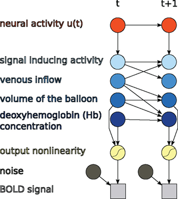
Figure 3. Hemodynamic forward model after discretization represented as a DBN, as used in this paper.

Discrete system of (13) can incorporate uncertainty of hemodynamic state variables X either through Euler–Maruyama (Kloeden and Platen, 1992) method or through the method of Jimenez et al. (1999). Different forms of discretization lead to different linearization filters (Johnston et al., 2008). For application of these methods to the differential equations system (8) see Riera et al. (2004) and Johnston et al. (2008).

Both linearization schemes are used together with adding noise to system variables, which reflects stochastic nature of the BOLD response generation. However, the main interest of our study is stochastic modeling of the hidden neural activity which is observed through noisy measurements of the BOLD response and MEG. Any reliable ODE solver suffices for our purposes and we assume noiseless signal generation by the forward model. In our model noise enters BOLD measurements on the sensor level only, as reflected by the diagram in Figure 3. Since the model returns the percentage of the BOLD response change the final fitting to the measured signal is done by:

where y(t) is the measurement at time t, η_t is zero-mean, unit-variance Gaussian noise, and σ ℬ and k are estimated parameters.

To integrate noiseless ODE equations in time we use the 4th order Runge–Kutta method. Thus the BOLD response generation model works deterministically with noise entering at the step of (14). This does not preclude the possibility of using a more sophisticated model, but still highlights stability issues and improvements brought by the joint analysis, as required for our study.

MEG forward model

We use the spherical head model of Sarvas (1987) for computing the magnetic field outside the head. The simplicity of its implementation and the speed of execution has made it a commonly used model among researchers in the field. Due to the findings of Hämäläinen and Sarvas (1989), which states that taking into account only the brain compartment for finding external magnetic field is as good as using a more complex brain–skull–scalp approximation, this model is widely used as sufficiently accurate model for magnetic field measurements.

For a dipole q at position r₀ inside the head, magnetic field outside the head at r is expressed as:

where F = a(ra + r² − r₀•r), a = r − r₀, a = |a|, r = |r| and ▽F = (r⁻¹a² + a⁻¹a•r + 2a + 2r)r − (a + 2r + a⁻¹a•r)r₀.

For the DBN model in this paper we are using a single active ROI. In the case of fMRI signal the ROI is modeled by the average activity of voxels comprising it. In the case of the spherical head model the ROI is represented by current dipoles located at the cortical surface of the ROI and oriented perpendicular to that surface. Since the locations and orientations of these dipoles are known from cortical geometry extracted by a segmentation algorithm, the lead field matrix can be precomputed. We additionally assume that dipoles of an ROI have equal magnitudes. This assumption significantly reduces the complexity of MEG forward model, since an anatomically detailed segmentation can return on the order of hundreds of thousands of dipoles per ROI. The final form of the forward model for MEG measurement due to activity of a single ROI is expressed by:

For N dipoles, M axial gradiometers, and K measurement coils, we compute K × (3N) lead field matrix L that depends on location and orientation of K measurement coils and location of N cortical dipoles. Vector o contains orientations of N cortical dipoles and has length 3N. W is the M × K switching matrix that transforms readings from the measurement coils into outputs of axial gradiometers. q is the scalar magnitude of the ROI (and each of its dipoles accordingly). Details of this formulation and matrix kernels for different MEG and EEG forward models can be found in (Mosher et al., 1999).

Particle Filtering

Particle filtering is a general approach to Bayesian filtering that allows handling of continuous random variables and non-linear transition and observation models (Doucet et al., 2001; Arulampalam et al., 2002). A particle filter is a Monte Carlo estimator of the posterior probability of a set of state variables for a system with general probability distributions over hidden variables and potentially non-linear dynamics. It uses a set of samples (called particles) to maintain a discrete estimate of a general probability distribution.

The technique has been recently applied to estimating the BOLD response and hemodynamic parameters using the hemodynamic forward model (Friston et al., 2003; Johnston et al., 2008). The conclusion was a superior performance of particle filtering comparing to extended Kalman filtering and a local linearization method. We are adopting particle filtering for our task of DBN inference for joint analysis of fMRI and MEG data.

The idea of particle filtering is based on the Monte Carlo histogram estimation. Given a set of samples from P(ℛ_t|𝒵_0:t), the distribution can be approximated with:

where δ(•) denotes the Dirac delta function. Using this we can approximate expectations of interest with

It is not easily possible to draw samples from P(ℛ_t|𝒵_0:t), so samples are generated from P(ℛ_0:t|𝒵_0:t). The task is accomplished through importance sampling (Liu, 2002; Mackay, 2002), by sampling from a proposal distribution Q and then weighting the particles with their importance ratio:

The recursive formulation of the problem leads to sequential algorithm that generates particles at the next time step and then weights them by the likelihood P(𝒵_t|ℛ_t).

It is required that the evolution of the hemodynamic model (see Hemodynamic Model) is computed at certain time intervals in order to maintain stability. In the sequential Monte Carlo framework propagation of the particles through the network (moving the fittest particles to the next time point and discarding the least fittest) needs to be controlled by the data likelihood P(𝒵_t|ℛ_t) from (19) in order to maintain sampling from highly likely regions of the distribution. It is desirable to have measurements available at each ODE integration step, so that the tracked hidden state can be brought in coherence with the data before drifting too far from the likely regions. However, fMRI measurements are only available every τ seconds, where τ is the length of the TR, which is too long for stability of the ODE system.

In order to satisfy requirements of ODE stability and data likelihood reweighting, we augment the model with both fMRI and MEG measurements simultaneously. High sampling rate of MEG guarantees availability of the data at a rate necessary to propagate the solution of the hemodynamic model. This framework (Figure 2) allows us to integrate MEG and fMRI data in a complementary way when the strength of both modalities are exploited.

When only fMRI is used to infer unobserved neural activity, we integrate the non-linear system of differential equations using sampling rate that provides a stable solution. However, resampling and reweighting is performed only at those integration points where the measurements are available. Thus most of the time the system performs stochastic search and is brought in coherence with the measurements only at the rate that corresponds to the sampling rate (TR) of the data. A particle smoother would be able to account for parts of these problems albeit incurring significantly larger computational resources, it would not be able to resolve the problem with the delay (discussed in greater detail later). We are not performing smoothing in this work for that reason and also because relative improvement of the fusion over fMRI-only results would remain when smoothing is uniformly applied over methods.

Results

First, we demonstrate our approach on a simulated dataset that exhibits the properties of the real data targeted by our model. Simulations provide known neural activity (i.e., ground truth) allowing us to characterize the performance of the approach: estimation behavior, stability of the estimate, and sensitivity to the noise. Next, we demonstrate the approach on a real fMRI/MEG dataset collected in two separate runs with the same visual event-related paradigm. Real data supports our findings confirming simulation-based observations. Although our model does not limit the exact form of connection between the hidden unit and the observed modalities, in this section we simply treat this activity as an appropriately scaled input to MEG forward model and its absolute value as the input to the HFM.

Simulation

In order to find out how estimation of neural activity and tracking of the BOLD response depends on the data modality and their combination, we have constructed the following simulation. We use the cortical surface extracted by FreeSurfer software (Fischl et al., 1999) from MRI of a human subject. A single ROI is selected from the FreeSurfer atlas: it is the bank of the superior temporal sulcus of the left hemisphere, shown in Figure 1. At this point the selection is arbitrary since for the simulation it does not make a difference, which ROI we select. Average fMRI activity of this ROI is generated by the hemodynamic forward model (Forward Models) from simulated neural activity formed by equally spaced weighted radial basis functions (RBF). In constructing simulation figures, we have expressed the BOLD signal as percentage of change around the baseline. Details of constructing simulated neural activity are described by Riera et al. (2004). Parameters of the HFM (see Table 1) were fixed to a value close to the average of the estimates from Riera et al. (2004). Parameters of the DBN model (k from Eq. 2 and noise variances) were estimated by a grid search on a hold out simulated data set, obtained using the input neural activity of Figure 5. The estimated values were used in the simulations and the real data application. The estimation could also be done without hold out data by using the EM algorithm (Dempster et al., 1977). The exact form of the underlying neural activity formed by RBF is shown by the line in the bottom plots of Figure 5. The hemodynamic forward model transformed this activity into the BOLD response, which is shown in the top plots of Figure 5 as the thin line. This activity was also used to generate the MEG signal for 273 axial gradiometers corresponding to CTF 275 system.

TABLE 1

Table 1. Parameters of the hemodynamic model.

In order to obtain physiologically correct measurements neural activity was scaled to have the maximum value of 50 nAm and treated as dipole magnitude q in Eq. 16. Noiseless simulated MEG measurements for 273 axial gradiometers are shown in Figure 4A. In simulations we set MEG sampling rate only four times higher than that of fMRI (2 Hz). It reduces computational burden and allows us to easily collect data from many experiments (e.g., Figure 7) and at the same time it reserves the main feature of the proposed fusion model: MEG contains more information about temporal dynamics of the neural activity than fMRI. Going to a higher sampling rate (as we do in real data experiments) only improves the situation since more information about temporal dynamics of the system gets represented. To create realistic conditions for MEG, we have added Gaussian noise to this output. Signal to noise ratio (SNR) of simulated MEG signal used in our experiments is set to −40 dB (see Figure 4B). We define the SNR as:

where 〈•〉 denotes the expected value, and A_i is an element of the signal (or noise) vector.

FIGURE 4

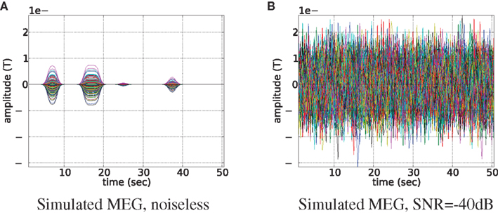
Figure 4. Magnetoencephalography signal generated by the uniformly active ROI (the bank of the superior temporal sulcus of the left hemisphere). Time courses of each of the 273 axial gradiometers are plotted on top of each other. Signal without noise is shown in subplot (A), and same signal but contaminated with noise of −40 dB is shown in subfigure (B).

We have applied and compared three different approaches to estimation of neural activity and tracking the BOLD response: using only simulated fMRI measurements (noise not added), using only simulated MEG measurements (−40 dB SNR), and using both measurements simultaneously. Figure 5 highlights the differences in the results.

FIGURE 5

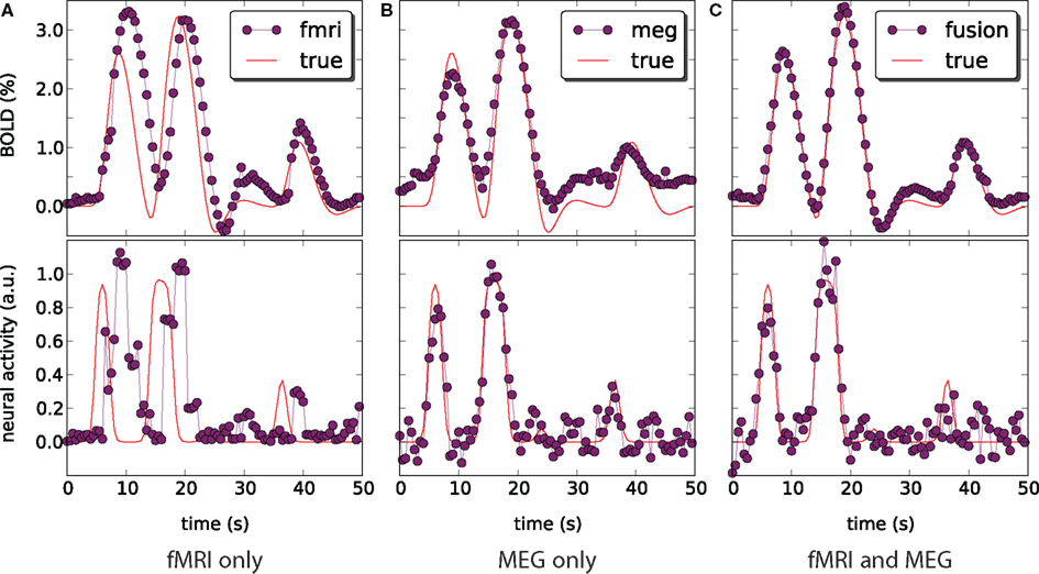
Figure 5. Blood oxygenation level dependent (top) and neural activity (bottom) signal plots. Each plot displays the ground truth signal (lines) plotted with the corresponding signal estimate produced by our Bayesian sensor fusion model (circles). Horizontal axes give time (seconds), while vertical axes are arbitrary units for neural activity and percent of change relative to baseline for BOLD. When the estimated curve falls close to the true curve, the model is performing well. (A) Displays estimation using only fMRI signal data; (B) displays estimation from only the MEG signal; while (C) shows the result of fusing both channels of data into a single estimate. We see that the fusion approach matches both the BOLD response and the neural activity more closely than do either of the single-channel estimates. Specifically, the fusion estimate tracks the BOLD response better than MEG and resolves a temporal ambiguity in the fMRI-only estimate. The temporal ambiguity corresponds to the hemodynamic delay, which is present as a parameter in our model. In (A,C) we have deliberately set the delay parameter to 0 to demonstrate that the fusion approach can use the MEG channel to resolve the hemodynamic delay without relying on a manually set parameter.

fMRI-only particle filtering loses track in the periods between available data points. To maintain a stable solution, differential equations need to be integrated with a time step smaller than the conventional TR of fMRI measurements (2 s in our case). This leads to stochastic evolution of the transition model not constrained by the data. This is visible in the BOLD response estimate of Figure 5A. The delay in the BOLD response generation is not captured by the default model (the shift is a parameter) and estimated neural activity is shifted in time (Figure 5A, bottom). In principle, this can be corrected in the particle filtering framework by using out of sequence particle filtering (Orton and Marrs, 2001; Mallick et al., 2002). We leave the delay uncorrected to demonstrate the effect of combined analysis.

MEG-only filtering is able to track neural activity with only some noise contaminating the estimate (MSE of 0.004). However, it is not tracking the BOLD response as good (Figure 5B), which is expected. The combined analysis corrects the shift in the estimate of neural activity as returned by fMRI-only filtering, improves the BOLD response tracking, and reduces the amount of noise in the neural activity estimate.

Qualitative analysis of Figure 5 demonstrates trends and differences in the signal tracking that yield the improved results seen in the combined analysis. The rest of this section concentrates on quantitative results for each of the advantages that the combined analysis provides over fMRI-only analysis.

An important improvement provided by the combined analysis is the decreased computational complexity of the filtering due to decrease in the number of particles needed. The more particles are used in the filter the better is the estimate of the posterior probability and hence of the quantities of interest. In the limit when number of particles goes to infinity the estimate is exact. For practical reasons, the number of particles should be as small as possible to enable fast computation while providing stable estimates.

For a fixed number of particles we can run the filtering procedure M times, compute an estimate Θ_m for each of the runs and compute its variance:

This variance can be used to control the influence of the number of particles on the estimate. Ideally one would want this variance to be close to 0. However, in practice it suffices to see it stabilize.

For fMRI-only and the combined analysis we compute the estimate of the mean and its variance with M = 800 for number of particles = 100k with k ∈{1,…,10}. Figure 6 demonstrates that fMRI-only filtering has much higher variance with the number of particles in the selected range and the variance is not stabilized even when 1000 particles are used. On the other hand the combined analysis provides stable results when number of particles is in the range [400,1000].

FIGURE 6

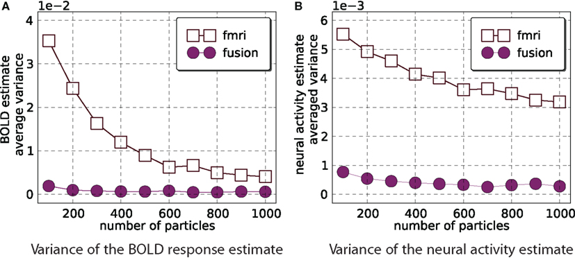
Figure 6. Estimator variance as a function of number of particles. This figure shows average (across all time points and 800 simulations) variance of estimated means of the BOLD response (A) and neural activity (B). Smaller values are better. It is clear that combined analysis requires much fewer particles to achieve lower variance of the estimate.

MEG and fMRI provide noisy measurements with typical SNR range of [−20,0] dB for MEG and [−15,5] dB for fMRI. In order to study how SNR of the measurements affects the combined analysis, the following simulation study was performed. For each of the simulated modalities SNR was varied in the range [−40,15] with a step size of 5. For each combination of SNR values for MEG and fMRI the filtering problem has been solved 20 times with different noise instantiation. The average MSE surfaces for the neural activity and the BOLD response estimates are shown in Figure 7. The algorithm is more sensitive to the SNR of fMRI than to SNR of MEG. In the range of typical SNRs the values of MSE have acceptable magnitude. MEG is shown to be less sensitive to the noise because we’re using a single ROI case and it is easier for the algorithms to handle Gaussian noise. We expect it to change in the multi-ROI case.

FIGURE 7

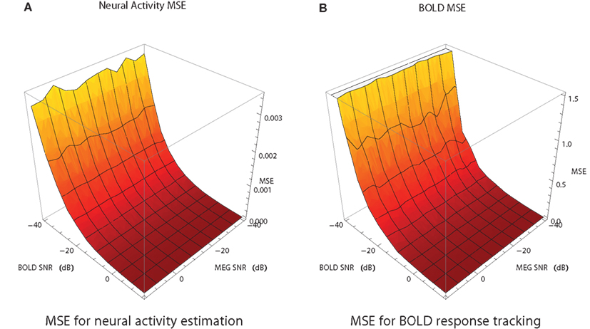
Figure 7. Mean squared error of the estimate of neural activity (A) and the BOLD response (B) as a function of SNR of fMRI and MEG data in the fMRI/MEG joint analysis. Each point is an average of 20 different runs, each with different noise instantiation and the random number generator seed.

Figures 6 and 7 use a fixed neural activity shape across all experiments. To study the effect of the input signal shape on the estimation, we have constructed a simulation in which signals of different density were generated. As previously, we are following the approach of Riera et al. (2004) by placing RBFs of equal standard deviation (σ = 0.02 s) at fixed equally spaced positions and weighting them. Now however we select weights from a zero-mean unit-variance Gaussian distribution (thus allowing negative weights) for a fixed number of RBFs keeping the rest 0. This allows us to control for the amount of neural activity. Figure 8 shows results in 1000 runs for each density level. For a total number of 70 allowed RBFs we have varied RBFs with non-zero weight from 10 to 70 with a step of 10. Resulting neural and corresponding BOLD signals typical for each density are shown in the middle pane. Each point on the figure is a root mean squared error (RMSE) normalized by the power of the true value and averaged over 1000 runs:

where ||•||₂ is the L₂-norm, T is the true signal and M is the model estimate. The fMRI estimated neural activity was manually shifted left by 4 s to decrease the effect of the default fMRI-only estimation of incorrectly identified lag (see Figure 5A) and provide some advantage to fMRI-only estimation. Note that MEG recovered the lag automatically and did not need such correction. Both approaches were compared to the absolute value of the input signal to keep the comparison on equal ground. The number of particles in the PF algorithm was set to 1000.

FIGURE 8

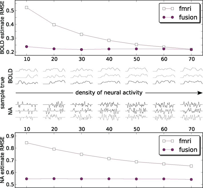
Figure 8. Estimation RMS error for BOLD (top) and neural activity (bottom) signals. Each point on the plot is an average of 1000 simulations each with its own ground truth. Neural activity becomes denser from left to right. To provide an idea what the signals look like the central panel shows a random sample of three true input and output signals 50 s in duration for each density. Data is available only at the markers (circles: fusion, squares: fMRI) – lines are for visual guides only. Estimates of both methods are compared to the absolute value of neural activity. fMRI estimates are shifted by the out of sequence parameter of −3 s to remove the harmful effect of incorrectly identified delay (Figure 5A).

Figure 8 shows that the combined analysis is more accurate for estimating neural activity as well as tracking the corresponding BOLD signal. As the power of neural activity grows, given the same maximum amplitude, the results of fMRI-only estimation improve. The low sampling rate of fMRI puts the system in disadvantage to the rapidly changing signals, since the estimate needs time to change the sign of the derivative. In the low density of neural activity many of such rapid changes of the bold response are happening, and fMRI-only system is confronted with a deliberately hard case. When many things are happening in the dense case they tend to flow smoother, which is especially pronounced for the smoothed BOLD response. This represent an easier case for fMRI-only estimation. However, it can be argued that, in practice, low density signals (in our definition) are encountered more often, for example in event-related paradigms.

The above simulations were done on (1) single-trial (non-averaged) data with (2) known parameters of the hemodynamic model, and, with exception of the noise sensitivity study, (3) noiseless BOLD data. Whereas noiseless BOLD (3) is an assumption well supported by our averaged experimental data of Section “Real Data Application,” the other two are not necessarily true. The single-trial analysis turns out to be very difficult in the real data due to the noise levels in MEG and ODE stability problems in the fMRI-only case. The parameters of the hemodynamic model can be estimated separately from neural activity tracking, for example, reported physiological values can be used (Friston et al., 2003). However, in general the parameters are unknown and need to be treated as states in the system.

We follow the literature with the joint estimation scheme where unscented Kalman filter (Zhenghui et al., 2009) and particle filter (Murray and Storkey, 2008) were successfully applied to simultaneous estimation of hemodynamic state variables and model parameters from the fMRI data. We have generated 7 s of simulated neural activity and the corresponding BOLD response in the time range with the sampling frequency of 1200 Hz (matching Section “Results”). The sampling rate was set the same for MEG and fMRI simulations, that mimics the averaged data of the real scenario, avoids stability issues in the fMRI-only case, and helps to match the statistical power of both modalities. Number of particles was set to 2000. Mean results of the fMRI-only and the joint estimates of neural activity and the BOLD response are shown in Figure 9.

FIGURE 9

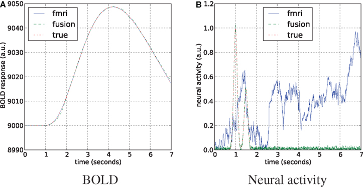
Figure 9. Estimation of the neural activity (B) and BOLD tracking (A) on simulated data with equal sampling rates for fMRI and MEG. The hemodynamic parameters are tracked as unknown states together with the unknown neural activity.

Both approaches perfectly follow the true BOLD response, although in the fMRI-only experiment neural activity is arbitrary. This happens due to the underdetermined nature of the system, where many different combinations of hemodynamic parameters and the neural activity can fit the data. In certain sense MEG is acting as a regularizer for this system, providing a good fit to BOLD and neural activity simultaneously.

The behavior of parameters across the tracking run for both approaches is summarized in Figure 10. The left column plots show a complete non-parametric representation of all distributions. The right column plots emphasize the differences by demonstrating important details, which may not be clearly visible on the box-plot due to differences in the parameter scale. The ratio of the inter quartile ranges (IQR) of fMRI-only to fusion experiment shows that for all parameters but the two (the neural efficacy and the resting oxygen extraction fraction) fMRI-only run produces significantly wider distributions of up to seven times for the hemodynamic transit time and the neural activity estimate. This is a clear demonstration of the underdetermined nature of the problem of inferring neural activity from the BOLD response. The PF algorithm using fMRI-only data allows the parameters to freely vary within a wide range while maintaining good fit to the data, whereas, in the case of fusion, parameters are constrained by MEG.

FIGURE 10

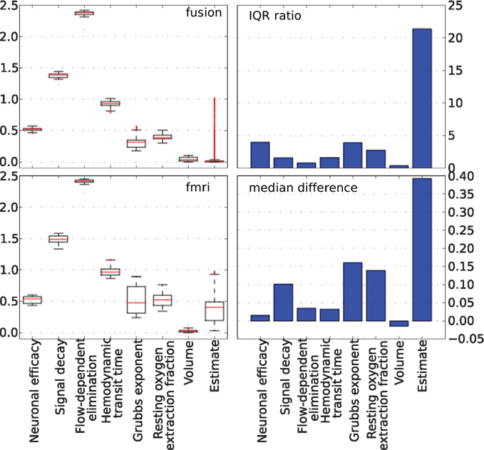
Figure 10. Non-parametric summary of parameter behavior by box and whisker (1. 5 IQR) and bar-plots comparing all parameters optimized by the PF on simulated data using fMRI-only vs. fusion data. These include seven hemodynamic parameters (Θ and V₀) and the estimate of neural activity. Bar-plots on the right summarize two important differences between results produced using fMRI-only and fusion data: ratio of IQR of fMRI over fusion, and difference of fMRI and fusion medians.

Figure 11 shows comparison of the median estimators with the true values of parameters from Table 1, where the fusion approach performs favorably (lower errors).

FIGURE 11

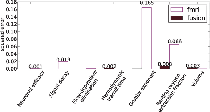
Figure 11. Squared errors of hemodynamic parameters: the estimated median values and the true values of Table 1.

Real Data Application

Validity of the simulation results is tested on visual stimulation data collected from a healthy adult male subject. Both MEG and fMRI modalities were collected using the same paradigm: 120 trials of an 8-Hz checkerboard reversal; each trial consisted of 1 s of 8 Hz oscillating checkerboard stimulus and 4 s ISI; with an additional 0–2 s of ISI randomly jittered (averaging out to 1 s of jitter).

Functional data were acquired at the remote site with EPI sequences on Siemens Avanto scanners at 1.5 Tesla (T). The imaging sequence parameters for these functional scans are as follow: Pulse sequence = single shot, single echo EPI, scan plane = oblique axial, AC-PC, copy T2 in-plane prescription, FOV = 240 mm, slice thickness = 3 mm, 1 mm skip, TR = 2000 ms, TE = 39 ms, FA = 90°, 64 × 64 matrix, 1 shot.

The MEG data was recorded with a VSMMedtech Omega 275 whole-head biomagnetometer system (VSM MedTech, Vancouver, BC, Canada) located at the Mind Research Network Imaging Center (Albuquerque, NM, USA). The data was recorded at 1200 samples/s, with only anti-aliasing filters applied. Post-processing included 60 HZ powerline noise removal.

Functional magnetic resonance imaging data were preprocessed using the SPM5 software package. Images were motion-corrected using INRIalign – an algorithm unbiased by local signal changes (Freire and Mangin, 2001; Freire et al., 2002). Data were spatially normalized into the standard Montreal Neurological Institute space (Friston et al., 1995) and slightly sub-sampled to 3 × 3 × 3 mm, resulting in 53 × 63 × 46 voxels. Next the data were spatially smoothed with a 10 × 10 × 10 mm full width at half-maximum Gaussian kernel. The resulting coordinates were converted to the Talairach and Tournoux standard space for anatomical mapping (Talairach and Tournoux, 1988).

MNE software (Hämäläinen, 2005) was used to localize cortical areas in the source space that are active while the task was performed. The areas that exhibited the most stimulus driven activity were identified from the expert knowledge of similar experiments, since visual stimulation mostly activates the primary visual cortex, (threshold levels set in MNE were 4.0, 8.5, and 9.5 for f_thresh, f_mid, and f_max parameters respectively) and corresponding ROIs from FreeSurfer (Fischl et al., 1999) atlas were chosen to represent the forward model (see Figure 12). A similar data collection scheme was used for EEG/fMRI fusion in (Ostwald et al., 2010). All dipoles orthogonal to the cortical surface and belonging to selected ROIs were used to construct the MEG forward model corresponding to the single hidden neural activity node in the DBN structure of Figure 2. The same ROIs were combined to build the HFM. This means that the model had single parameter for dipole amplitude (the same for all dipoles) in the MEG forward model and the absolute value parameter (with appropriate scaling) was also used as neural activity in the fMRI forward model. The activity source in the real data experiment is localized and active voxels do not differ substantially in their dynamics to cause problems when averaging.

FIGURE 12

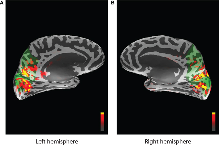
Figure 12. Activity localized by the MNE software inverse solution and overlayed on the inflated cortical surface. Peak stimulus driven activity is shown by red and yellow colors. Green areas indicate the region selected from the FreeSurfer atlas and corresponding to cuneus, precuneus, and pericalcarine ROIs for the left (A) and the right (B) hemispheres.

The data for both modalities were averaged with reference to the stimulus onset, discarding the first and the last 10 s of the run. fMRI data was linearly interpolated to the MEG resolution (1200 Hz) before averaging (see Figure 13) . Although it is a different setup from what was used in simulations and it leads to sample-by-sample symmetric treatment of both modalities, fMRI information content is not increased by interpolation and MEG still provides the most information about the dynamics of the latent activity. The averaging of fMRI time courses was performed over all of the voxels belonging to cuneus, precuneus, and pericalcarine ROIs of the FreeSurfer atlas.

FIGURE 13

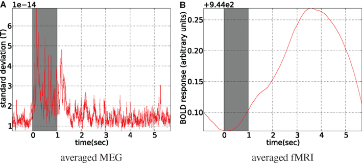
Figure 13. Stimulus-locked averaged data. Stimulus presentation is shown with the gray bar from 0 to 1 s, where 8 Hz flashing checkerboard was presented. fMRI was linearly interpolated to MEG sampling rate (1200 Hz) before averaging (A). For MEG spatial standard deviation in the sensor space is shown (B), (the global field power).

A substantial difference between our simulations and application of the method to the real dataset is the unknown parameters of the hemodynamic forward model. In this experiment we have treated them as additional random variables independent of each other and evolving as part of the original DBN model with prior values from Table 1. This corresponds to the “artificial evolution” of parameters concept in sequential Monte Carlo literature (Doucet et al., 2001) and was previously applied to fMRI data (Murray and Storkey, 2008) filtering. Thus we are able to treat unknown parameters of the HFM together with estimating neural activity and tracking the BOLD response under the framework of DBNs. Since the state space increased when parameters were added, we have increased the number of particles to 2000 (an empirical estimate that produced consistent results) to better capture the posterior.

The results of application of our method to the real data are displayed in Figure 14. They are presented in the same manner as the simulation results of Figure 5. The gray strip signifies the interval at which the flashing checkerboard stimulus was presented. fMRI-only estimation in Figure 14A is able to track the data (the BOLD response) almost perfectly. However, it produces a noisy neural activity estimate. Although it does increase together with the data similarly as observed in simulations. Note, that when estimation of neural activity is performed together with estimating the system’s parameters we are dealing with an underdetermined system, i.e., many different solutions fit the objective perfectly and we are left with inverse problem (Riera et al., 2004). We attribute poor performance of the fMRI-only estimation to this inverse problem. MEG-only estimation is quite opposite: it estimates the neural activity consistently with the stimulus presentation (Figure 14B) and fails at tracking the data. This happens since the MEG-only estimation is unconstrained by the fMRI data and, obviously, HFM parameters freely drift away from the solution region. Results of the joint analysis of MEG and fMRI (Figure 14C) support our findings in the simulated experiments: fMRI data is traced exactly and neural activity is estimated as expected. Figure 14 displays neural activity as the absolute value of the estimate, the way it inputs the HFM.

FIGURE 14

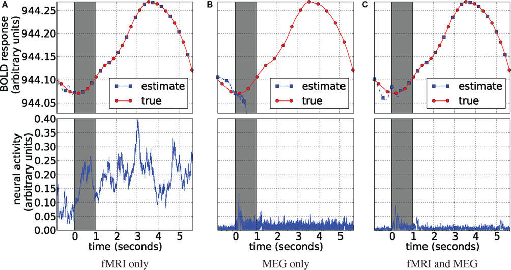
Figure 14. Blood oxygenation level dependent (top) and neural activity (bottom) estimation plots. Each plot displays the averaged BOLD response (red circles) plotted with the corresponding signal estimate produced by our Bayesian sensor fusion model (blue squares). Since true neural activity is not known for the real dataset only the estimate is displayed in the bottom plots. Horizontal axes give time (seconds), while vertical axes are arbitrary units for signal response. The BOLD response is perfectly tracked by fMRI (A) as well as by the joint analysis (C). However, MEG completely fails to track it. fMRI-only analysis fails to track neural response (B). In both cases this is due to varying parameters of the HFM, required since the true parameters are unknown. This lead to underdetermined problem in case of fMRI, creating random results while maintaining perfect fit, and also allowed the MEG-only case to drift off completely, since it was not constrained by the BOLD response. The joint analysis is closely tracking the BOLD response and provides neural activity estimation consistent with expectation from previous knowledge about the experiment (C).

As noted previously, in all real data experiments all hemodynamic parameters were modeled as random variables. They were tracked by PF together with the neural activity. A summary of the behavior of these parameters is presented in Figure 15, together with the estimate of the neural activity for completeness. The MEG-only experiment is not shown since the hemodynamic model was completely unconstrained in that case. The information presented in the figure matches that of Figure 10 and the results are generally similar to the simulated data case. The bar-plot of the differences in medians between fusion and fMRI-only runs demonstrates that parameter values in the fusion case are generally lower (negative values). A possible explanation would be the types of local minima that the unconstrained inference of fMRI-only case tends to follow, require higher values of the parameters to maintain the fit. We conclude that our fusion approach with further work can be user for inference of hemodynamic parameters as an application alternative to neural activity inference.

FIGURE 15

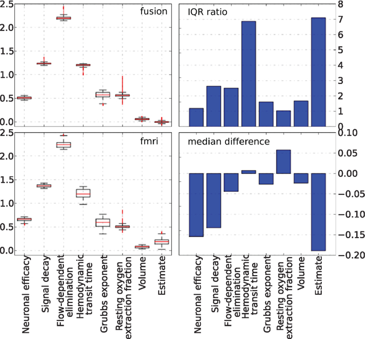
Figure 15. Non-parametric summary of parameter behavior by box and whisker (1. 5 IQR) and bar-plots comparing all parameters optimized by the PF on real data using fMRI-only vs. fusion data. These include seven hemodynamic parameters (Θ and V₀) and the estimate of neural activity. Bar-plots on the right summarize two important differences between results produced using fMRI-only and fusion data: ratio of IQR of fMRI over fusion, and difference of fMRI and fusion medians.

Discussion

Inference of neural activity in a single ROI from its BOLD signal has been implemented previously in the context of non-linear optimization by Vakorin et al. (2007), and in the context of the state space models (Riera et al., 2004; Deneux and Faugeras, 2006; Johnston et al., 2008), which are a special case of DBNs. By generalizing the problem to stochastic inference of neural activity in the DBN framework, we gain additional benefits of probabilistic modeling, such as the ability to use different transition and observation models without significant changes to algorithms, and the ability to combine measurements from different modalities. For example, EEG can be either easily added to the two already used modalities or can replace MEG, if MEG measurements are not available or in the case of concurrent EEG–fMRI recordings. Concurrent recordings ultimately yield the most suitable experimental data for our method. Another important consequence of the generalization is the ability to handle more than one ROI.

We improve estimation of the dynamics of the neural activity of an ROI in order to guarantee improvements in the modeling of statistical dependencies among multiple ROIs in future work. Currently in the DBN framework this is done by using fMRI-only analysis assuming that ROIs are directly observed (Zhang et al., 2006; Burge et al., 2007; Rajapakse and Zhou, 2007), which ignores indirect nature of the observations and makes it harder to add observations from other modalities. DBNs are general in their ability to support a wide class of dependency structures among hidden variables. Observations are not restricted to come from particular ROIs or happen always at a fixed time. Structural information of a DBN can provide interesting information about underlying problem. This ability can be important for modeling the brain’s functional connectivity.

The seeming coarseness of the uniformly active ROI is not an issue for the relationship (network) analysis. Even though there can be several possible dipole configurations within each ROI supporting the same MEG measurements, their temporal dynamics averaged across ROI will have to be very similar to support the dynamics of the measurements and fMRI predicted dynamics of the ROI. After all, ROI based approaches are widely adopted in the fMRI research field.

Different forward models would give us benefits in either computation time (as in the case of fMRI models developed using the theory of linear time invariant systems (LTIS)) or precision (in case of using a finite element model (FEM) for MEG). However, our choice was determined by desire to have simple and yet dynamically accurate models. As experiments demonstrate, these models fit the task well. Further discussion of forward modeling for MEG and fMRI can be found in Halchenko et al. (2005).

When the notion of inverse problem is brought up in the context of electromagnetic modeling it is commonly assumed that the problem at hand is the problem of localizing the sources in space (Hämäläinen et al., 1993). This notion is reflected in the focus on localization in many studies of simultaneous analysis of MEG, fMRI, and EEG (Dale and Sereno, 1993; Dale et al., 2000; Friston et al., 2008; Jun et al., 2008). Even the general variational Bayesian approach of Daunizeau et al. (2007) which pays significant attention to dynamics of the signal still connects the modalities through their spatial profile thus putting more emphasis on the spatial inverse problem. At the same time, temporal inverse problem becomes important in the real data analysis of fMRI signals (Riera et al., 2004), when hemodynamic parameters are unknown. This paper focuses mainly on the temporal aspects (see causality arguments below) and emphasizes the temporal inverse problem. Our study provides evidence that MEG (or EEG) can be used to simultaneously constrain neural activity and HFM parameter estimation mitigating consequences of the fMRI inverse problem. Figures 14A,C provide different estimates of neural activity due to constraints introduced by MEG data. This reduces the degrees of freedom of the system which may lead to better estimates of HFM parameters. Unfortunately, the large number of parameters of the HFM makes it hard to completely determine the system by simply adding an extra data source to the fMRI-only estimate. The system still is highly underdetermined and additional parameter restrictions should be employed if one is specifically interested in the true parameter values and not as much in the neural activity tracking. Addition of MEG constraints the system to stay in the nearest basin of parameter values is able to satisfy simultaneous fit ob the BOLD and MEG data. This does improve tracking results considerably (given that fMRI-only does not provide a sensible result in this case). However, if no prior information about parameter values is available parameters may end up in a wrong basin of attraction, and/or the system may experience oscillatory behavior before a satisfying assignment is found (for example see Figure 14C). Nevertheless, we feel that the fusion approach for parameter estimation is promising. The symmetric mutual constraining of MEG and fMRI is different from existing approaches (Dale et al., 2000; Jun et al., 2008), where fMRI is used as a prior to MEG, and from data-driven approaches, which identify mutual co-variation between hemodynamic and electrical signals (Calhoun et al., 2006; Eichele et al., 2008), but don’t employ a model of the dynamic relationship between the two.

Another motivation for emphasizing the temporal component and exploiting as much temporal information as available is related to causality. As it has been previously noted, reliance on either bioelectric or hemodynamic signals may lead to opposite conclusions regarding causality (Daunizeau et al., 2007). Our ultimate motivation being brain’s effective connectivity, this is an important call to focus on temporal aspects of the hidden signal.

Our fusion framework as formulated in the context of DBNs (Dynamic Model) is very general and potentially can account for all approaches discussed by Valdes-Sosa et al. (2009). In this paper at the forward modeling stage neural activity enters the MEG forward model after an appropriate scaling and the fMRI forward model after the sign correction, as explained in Section “Results.” It may seem as if we bias the model toward the asymmetric case in the classification of (Valdes-Sosa et al., 2009), but this is not the case. It becomes clear from the real data experiment case, where at each time point possible solutions are weighted according to both modalities and neither is given more weight a priori. The resulting time course is a combination of evidence from all available modalities simultaneously. A similar approach of linking the modalities together was implemented by Daunizeau et al. (2007) only focusing on spatial rather than temporal aspects. Another difference with our work is the disparity of the data collection intervals analyzed by the algorithm. In Daunizeau et al. (2007) about 50 ms of collected MEG and about 900 s of fMRI were visible to the algorithm, whereas we are performing the tracking in parallel in the same time interval.

In principle our DBN model formulation supports incorporation of complicated models connecting post synaptic potentials with the observed BOLD response and MEG signal (Babajani and Soltanian-Zadeh, 2006; Riera et al., 2006, 2007; Valdes-Sosa et al., 2009), but we have resorted to a much simpler statistical model. Our motivation follows that of Daunizeau et al. (2007), it is hard to choose the right forward model when the relationship is not fully understood. As our results show, a simple model can also lead to valuable results. In future work it may be valuable to incorporate models with greater physiological motivation.

Particle filtering has been previously applied to analyzing MEG data (Somersalo et al., 2003; Campi et al., 2008) and the BOLD response (Johnston et al., 2008; Murray and Storkey, 2008). The goal in the first case was to solve the electromagnetic inverse problem by tracking unobserved current dipoles as sources of MEG measurements. In the BOLD response case it was tracking the underlying signal as well as the response and hemodynamic parameters. To the best of our knowledge, we are the first to use PF in combining these modalities. As shown in extensive simulations by Johnston et al. (2008) PF are accurate, robust and efficient compared to linearization-based techniques. This is confirmed for the most part by comparison to a more recent expectation maximization based model (Friston et al., 2008). The only case were PF did not perform that well was the case of a system exhibited deterministic chaos behavior, as shown by Friston et al. (2008). Our method should be applied with caution in such cases since it may not be the best choice or even applicable.

The flexibility of the PF framework is usually counterbalanced by the difficulties it can have when dealing with large scale problems. These include computational and storage resources required to satisfactorily track the growing number of particles needed when the dimensions of the problem grow. An approach similar to ours (Murray and Storkey, 2008), when used to analyze statistical dependencies among multiple ROIs requires considerable computational resources. The algorithm is run on a parallel cluster in order to handle propagation of 1e6 particles. This is only for 4 ROIs and linear dependencies among particles. An interesting outcome of our work is a substantial decrease in these requirements achieved by fusion compared to fMRI-only analysis (see Figure 6). We expect this to be an advantage for multi-ROI analysis. Research of exploiting the special structure of the DBN (e.g., a single BOLD observation per hidden ROI), also allows us greatly decrease the complexity of PF framework. Mathematical details of this new advance are shown in (Besada-Portas et al., 2009). These advances form the basis of our future work in the current direction.

Conclusions

We have presented a way to perform joint analysis of fMRI and MEG data for inferring latent neural activity and tracking the BOLD response in the framework of DBNs. Non-linear state estimation and tracking was performed using particle filtering framework. Simulations and real data results demonstrate the advantages of combining fMRI and MEG: improved tracking of the dynamics of neural activity, automatic control for signal delay properties of the BOLD response, increase in SNR of the estimate, improved computational properties of the system due to fewer required particles, improved stability of the differential equations in the HFM, and possibility of mitigating the consequences of inverse problem when HFM parameter estimation is required. Future work will extend the approach to other modalities (EEG) and to multiple ROIs as well as employing inferred neural activity to estimate the functional connectivity in the brain.

Acknowledgments

This research was supported by NIMH grant 1 R01 MH076282-01 as part of the NSF/NIH Collaborative Research in Computational Neuroscience Program and in part by the National Institutes of Health, under grants 1 R01 EB 006841, 1 R01 EB 005846, 5 P20 RR 021938 (Vince D. Calhoun) and a grant from the L. Meltzer University fund 801616 (Tom Eichele). Parts of the work were funded by 5R21MH069965-02 to Michael P. Weisend and DARPA Contract NBCHC070103 to Vincent P. Clark and The Mind Research Network. We thank the research staff at the Mind Research Network who helped collect and process the data: Dae Il Kim, Mark Scully, Judith Segall, and Matthew Euler.

Conflict of Interest Statement

The authors declare that the research was conducted in the absence of any commercial or financial relationships that could be construed as a potential conflict of interest.

References

Arulampalam, S., Maskell, S., Gordon, N., and Clapp, T. (2002). A tutorial on particle filters for on-line non-linear/non-Gaussian Bayesian tracking. IEEE Trans. Signal Process. 50, 174–188.

Babajani, A., and Soltanian-Zadeh, H. (2006). Integrated MEG/EEG and fMRI model based on neural masses. IEEE Trans. Biomed. Eng. 53, 1794–1801.

Pubmed Abstract | Pubmed Full Text

Bertrand, C., Ohmi, M., Suzuki, R., and Kado, H. (2001). A probabilistic solution to the MEG inverse problem via MCMC methods: the reversible jump and parallel tempering algorithms. IEEE Trans. Biomed. Eng. 48, 533–542.

Pubmed Abstract | Pubmed Full Text

Besada-Portas, E., Plis, S., de la Cruz, J., and Lane, T. (2009). “Parallel subspace sampling for particle filtering in dynamic Bayesian networks,” in Machine Learning and Knowledge Discovery in Databases, Vol. 5781, Lecture Notes in Computer Science, eds W. Buntine, M. Grobelnik, D. Mladenic, and J. Shawe-Taylorpages (Berlin/Heidelberg: Springer), 131–146.

Bießmann, F., Meinecke, F. C., Gretton, A., Rauch, A., Rainer, G., Logothetis, N. K., and Müller, K. R. (2010). Temporal kernel CCA and its application in multimodal neuronal data analysis. Mach. Learn. 79, 5–27.

Burge, J., Lane, T., Link, H., Qiu, S., and Clark, V. P. (2007). Discrete dynamic Bayesian network analysis of fMRI data. Hum. Brain Mapp. 30, 122–137. ISSN 1065-9471.

CrossRef Full Text

Buxton, R. B., Wong, E. C., and Frank, L. R. (1998). Dynamics of blood flow and oxygenation changes during brain activation: the balloon model. Magn. Reson. Med. 39, 855–864.

Pubmed Abstract | Pubmed Full Text

Calhoun, V. D., Adali, T., Pearlson, G. D., and Kiehl, K. A. (2006). Neuronal chronometry of target detection: fusion of hemodynamic and event-related potential data. Neuroimage 30, 544–553.

Pubmed Abstract | Pubmed Full Text | CrossRef Full Text

Campi, C., Pascarella, A., Sorrentino, A., and Piana, M. (2008). A Rao-Blackwellized particle filter for magnetoencephalography. Inverse Probl. 24, 25023–25037.

CrossRef Full Text

Dale, A. M., Liu, A. K., Fischl, B. R., Buckner, R. L., Belliveau, J. W., Lewine, J. D., and Halgren, E. (2000). Dynamic statistical parametric mapping combining fMRI and MEG for high-resolution imaging of cortical activity. Neuron 26, 55.

Pubmed Abstract | Pubmed Full Text | CrossRef Full Text

Dale, A. M., and Sereno, M. I. (1993). Improved localizadon of cortical activity by combining EEG and MEG with MRI cortical surface reconstruction: a linear approach. J. Cogn. Neurosci. 5, 162–176.

Daunizeau, J., Grova, C., Marrelec, G., Mattout, J., Jbabdi, S., Pélégrini-Issac, M., Lina, J. M., and Benali, H. (2007). Symmetrical event-related EEG/fMRI information fusion in a variational Bayesian framework. Neuroimage 36, 69–87.

Pubmed Abstract | Pubmed Full Text | CrossRef Full Text

Dempster, A. P., Laird, N. M., and Rubin, D. B. (1977). Maximum likelihood from incomplete data via the EM algorithm. J. R. Stat. Soc. B (Methodol.) 39, 1–38.

Deneux, T., and Faugeras, O. (2006). “EEG-fMRI fusion of non-triggered data using Kalman filtering,” in Biomedical Imaging: Nano to Macro, 2006. Third IEEE International Symposium on April 2006, Arlington, VA, 1068–1071.

Doucet, A., de Freitas, N., and Gordon, N. (eds). (2001). Sequential Monte Carlo Methods in Practice. Berlin: Springer-Verlag.

Eichele, T., Calhoun, V. D., Moosmann, M., Specht, K., Jongsma, M. L. A., Quiroga, R. Q., Nordby, H., and Hugdahl, K. (2008). Unmixing concurrent EEG-fMRI with parallel independent component analysis. Int. J. Psychophysiol. 67, 222–234.

Pubmed Abstract | Pubmed Full Text | CrossRef Full Text

Eichele, T., Specht, K., Moosmann, M., Jongsma, M. L. A., Quiroga, R. Q., Nordby, H., and Hugdahl, K. (2005). Assessing the spatiotemporal evolution of neuronal activation with single-trial event-related potentials and functional MRI. Proc. Natl. Acad. Sci. U.S.A. 102, 17798.

Pubmed Abstract | Pubmed Full Text | CrossRef Full Text

Fischl, B., Sereno, M. I., and Dale, A. M. (1999). Cortical surface-based analysis. II: Inflation, flattening, and a surface-based coordinate system. Neuroimage 9, 195–207.

Pubmed Abstract | Pubmed Full Text | CrossRef Full Text

Freire, L., and Mangin, J. F. (2001). Motion correction algorithms may create spurious brain activations in the absence of subject motion. Neuroimage 14, 709–722.

Pubmed Abstract | Pubmed Full Text | CrossRef Full Text

Freire, L., Roche, A., and Mangin, J. F. (2002). What is the best similarity measure for motion correction in fMRI. IEEE Trans. Med. Imaging 21, 470–484.

Pubmed Abstract | Pubmed Full Text

Friston, K. J., Ashburner, J., Frith, C. D., Poline, J. B., Heather, J. D., and Frackowiak, R. S. J. (1995). Spatial registration and normalization of images. Hum. Brain Mapp. 3, 165–189.

CrossRef Full Text

Friston, K. J., Harrison, L., and Penny, W. (2003). Dynamic causal modelling. Neuroimage 19, 1273–1302.

Pubmed Abstract | Pubmed Full Text | CrossRef Full Text

Friston, K. J., Mechelli, A., Turner, R., and Price, C. J. (2000). Nonlinear responses in fMRI: the Balloon model, Volterra kernel, and other hemodynamics. Neuroimage 12, 466–477.

Pubmed Abstract | Pubmed Full Text | CrossRef Full Text

Friston, K. J., Trujillo-Barreto, N., and Daunizeau, J. (2008). DEM: a variational treatment of dynamic systems. Neuroimage 41, 849–885.

Pubmed Abstract | Pubmed Full Text | CrossRef Full Text

Gelman, A., Carlin, J. B., Stern, H. S., and Rubin, D. B. (2003). Bayesian Data Analysis, 2nd Edn. Boca Raton: Chapman & Hall/CRC. ISBN 158488388X.

Halchenko, Y. O., Hanson, S. J., and Pearlmutter, B. A. (2005). “Multimodal integration: fMRI, MRI, EEG, and MEG (chapter 8),” in Signal Processing and Communications, eds L. Landini, V. Positano, and M. F. Santarelli (New York, NY: Marcel Dekker), 223–265. ISBN 0824725425.

Hämäläinen, M. S. (2005). MNE Software User’s Guide. Available at http://www.nmr.mgh.harvard.edu/martinos/userInfo/data/sofMNE.php

Hämäläinen, M. S., Hari, R., Ilmoniemi, R. J., Knuutila, J., and Lounasmaa, O. V. (1993). Magnetoencephalography: theory, instrumentation, and applications to noninvasive studies of the working human brain. Rev. Mod. Phys. 65, 413–497.

Hämäläinen, M. S., and Sarvas, J. (1989). Realistic conductivity geometry model of the human head for interpretation of neuromagnetic data. IEEE Trans. Biomed. Eng. 36, 165–171.

Huettel, S. A., Song, A. W., and McCarthy, G. (2004). Functional Magnetic Resonance Imaging. Sunderland, MA: Sinauer Associates, Publishers. ISBN 0-87893-288-7.

Jimenez, J. C., Shoji, I., and Ozaki, T. (1999). Simulation of stochastic differential equations through the local linearization method. A comparative study. J. Stat. Phys. 94, 587.

Johnston, L. A., Duff, E., Mareels, I., and Egan, G. F. (2008). Nonlinear estimation of the bold signal. Neuroimage 40, 504–514.

Pubmed Abstract | Pubmed Full Text | CrossRef Full Text

Jun, S.-C., George, J. S., Kim, W., Paré-Blagoev, J., Plis, S., Ranken, D. M., and Schmidt, D. M. (2008). Bayesian brain source imaging based on combined MEG/EEG and fMRI using MCMC. Neuroimage 40, 1581–1594.

Pubmed Abstract | Pubmed Full Text | CrossRef Full Text

Jun, S.-C., George, J. S., Pare-Blagoev, J., Plis, S. M., Ranken, D. M., Schmidt, D. M., and Wood, C. C. (2005). Spatiotemporal Bayesian inference dipole analysis for MEG neuroimaging data. Neuroimage 28, 84–98.

Pubmed Abstract | Pubmed Full Text | CrossRef Full Text

Kloeden, P. E., and Platen, E. (1992). Numerical Solution of Stochastic Differential Equations. Berlin: Springer.

CrossRef Full Text

Liu, J. S. (2002). Monte Carlo Strategies in Scientific Computing. New York: Springer. ISBN 0387952306.

Logothetis, N. K., and Wandell, B. A. (2004). Interpreting the bold signal. Annu. Rev. Physiol. 66, 735–769.

Pubmed Abstract | Pubmed Full Text | CrossRef Full Text

Mackay, D. J. C. (2002). Information Theory, Inference and Learning Algorithms. Cambridge: Cambridge University Press. ISBN 0521642981.

Mallick, M., Kirubarajan, T., and Arulampalam, S. (2002). “Out-of-sequence measurement processing for tracking ground target using particle filters,” in Aerospace Conference Proceedings, 2002, Vol. 4 (IEEE), 1809–1818. Available at http://ieeexplore.ieee.org/xpls/abs_all.jsp?arnumber=1036893

CrossRef Full Text

Mandeville, J. B., Marota, J. J., Ayata, C., Zaharchuk, G., Moskowitz, M. A., Rosen, B. R., and Weisskoff, R. M. (1999). Evidence of a cerebrovascular postarteriole windkessel with delayed compliance. J. Cereb. Blood Flow Metab. 19, 679–689. ISSN 0271-678X.

Pubmed Abstract | Pubmed Full Text | CrossRef Full Text

Moosmann, M., Eichele, T., Nordby, H., Hugdahl, K., and Calhoun, V. D. (2008). Joint independent component analysis for simultaneous EEG-fMRI: principle and simulation. Int. J. Psychophysiol. 67, 212–221.

Pubmed Abstract | Pubmed Full Text | CrossRef Full Text

Mosher, J. C., Leahy, R. M., and Lewis, P. S. (1999). EEG and MEG: forward solutions for inverse methods. IEEE Trans. Biomed. Eng. 46, 245–259. ISSN 0018-9294.

Pubmed Abstract | Pubmed Full Text

Mukamel, R., Gelbard, H., Arieli, A., Hasson, U., Fried, I., and Malach, R. (2005). Coupling between neuronal firing, field potentials, and fMRI in human auditory cortex. Science 309, 951–954.

Pubmed Abstract | Pubmed Full Text | CrossRef Full Text

Murphy, K. (2002). Dynamic Bayesian Networks: Representation, Inference and Learning. Ph.D. thesis, UC Berkeley.

Murray, L., and Storkey, A. (2008). “Continuous time particle filtering for fMRI,” in Advances in Neural Information Processing Systems, Vol. 20, eds J. C. Platt, D. Koller, Y. Singer, and S. Roweis (Cambridge, MA: MIT Press), 1049–1056.

Obata, T., Liu, T. T., Miller, K. L., Luh, W.-M., Wong, E. C., Frank, L. R., and Buxton, R. B. (2004). Discrepancies between bold and flow dynamics in primary and supplementary motor areas: application of the balloon model to the interpretation of bold transients. Neuroimage 21, 144.

Pubmed Abstract | Pubmed Full Text | CrossRef Full Text

Orton, M., and Marrs, A. (2001). “A Bayesian approach to multi-target tracking and data fusion with out-of-sequence measurements,” in Target Tracking: Algorithms and Applications (Ref. No. 2001/174), Vol. 1 (IEEE), 15/1–15/5.

CrossRef Full Text

Ostwald, D., Porcaro, C., and Bagshaw, A. P. (2010). An information theoretic approach to EEG-fMRI integration of visually evoked responses. Neuroimage 49, 498–516. ISSN 1053-8119.

Pubmed Abstract | Pubmed Full Text | CrossRef Full Text

Rabiner, L. R. (1989). A tutorial on hidden Markov models and selected applications in speech recognition. Proc. IEEE 77, 257–286. ISSN 0018-9219.

CrossRef Full Text

Raichle, M. E., and Mintun, M. A. (2006). Brain work and brain imaging. Annu. Rev. Neurosci. 29, 449–476.

Pubmed Abstract | Pubmed Full Text

Rajapakse, J. C., and Zhou, J. (2007). Learning effective brain connectivity with dynamic Bayesian networks. Neuroimage 37, 749–760.

Pubmed Abstract | Pubmed Full Text | CrossRef Full Text

Riera, J. J., Jimenez, J. C., Wan, X., Kawashima, R., and Ozaki, T. (2007). Nonlinear local electrovascular coupling. II: from data to neuronal masses. Hum. Brain Mapp. 28, 335–354.

Pubmed Abstract | Pubmed Full Text | CrossRef Full Text

Riera, J. J., Wan, X., Jimenez, J. C., and Kawashima, R. (2006). Nonlinear local electro-vascular coupling. Part I: a theoretical model. Hum. Brain Mapp. 27, 896–914.

Pubmed Abstract | Pubmed Full Text | CrossRef Full Text

Riera, J. J., Watanabe, J., Kazuki, I., Naoki, M., Aubert, E., Ozaki, T., and Kawashima, R. (2004). A state-space model of the hemodynamic approach: nonlinear filtering of BOLD signals. Neuroimage 21, 547–567. ISSN 1053-8119.

Pubmed Abstract | Pubmed Full Text | CrossRef Full Text

Sarvas, J. (1987). Basic mathematical and electromagnetic concepts of the biomagnetic inverse problem. Phys. Med. Biol. 32, 11–22.

Pubmed Abstract | Pubmed Full Text

Schmidt, D. M., George, J. S., and Wood, C. C. (1999). Bayesian inference applied to the electromagnetic inverse problem. Hum. Brain Mapp. 7, 195–212.

Pubmed Abstract | Pubmed Full Text | CrossRef Full Text

Sekihara, K., Nagarajan, S. S., Poeppel, D., Marantz, A., and Miyashita, Y. (2001). Reconstructing spatio-temporal activities of neural sources using an MEG vector beamformer technique. IEEE Trans. Biomed. Eng. 48, 760–771.

Pubmed Abstract | Pubmed Full Text

Somersalo, E., Voutilainen, A., and Kaipio, J. P. (2003). Non-stationary magnetoencephalography by Bayesian filtering of dipole models. Inverse Probl. 19, 1047–1063.

CrossRef Full Text

Stephan, K. E., Weiskopf, N., Drysdale, P. M., Robinson, P. A., and Friston, K. J. (2007). Comparing hemodynamic models with DCM. Neuroimage 38, 387–401.

Pubmed Abstract | Pubmed Full Text | CrossRef Full Text

Talairach, J., and Tournoux, P. (1988). Co-planar Stereotaxic Atlas of the Human Brain: 3-Dimensional Proportional System: An Approach to Cerebral Imaging. New York: Thieme.

Pubmed Abstract | Pubmed Full Text

Vakorin, V. A., Krakovska, O. O., Borowsky, R., and Sarty, G. E. (2007). Inferring neural activity from bold signals through nonlinear optimization. Neuroimage 38, 248.

Pubmed Abstract | Pubmed Full Text | CrossRef Full Text

Valdes-Sosa, P. A., Sanchez-Bornot, J. M., Sotero, R. C., Iturria-Medina, Y., Aleman-Gomez, Y., Bosch-Bayard, J., Carbonell, F., Ozaki, T., Center, C. N., and Havana, C. (2009). Model driven/fMRI fusion of brain oscillations. Hum. Brain Mapp. 30, 2701–2721.

Pubmed Abstract | Pubmed Full Text | CrossRef Full Text

Zhang, L., Samaras, D., Alia-Klein, N., Volkow, N., and Goldstein, R. (2006). “Modeling neuronal interactivity using dynamic Bayesian networks,” in Advances in Neural Information Processing Systems, Vol. 18, eds Y. Weiss, B. Schölkopf, and J. Platt (Cambridge, MA: MIT Press), 1593–1600.

Zhenghui, H., Xiaohu, Z., Huafeng, L., and Pengcheng, S. (2009). Nonlinear analysis of the bold signal. EURASIP J. Adv. Signal Process. 2009, 13. doi:10.1155/2009/215409.