NeuroMap: a spline-based interactive open-source software for spatiotemporal mapping of 2D and 3D MEA data

Introduction

Microelectrode arrays (MEAs) are a powerful tool to record large populations of neurons and monitor local neural networks as a whole. They are increasingly employed in a wide variety of studies, in vivo (Nicolelis et al., 1997; Csicsvari et al., 2003) as well as in vitro (Shahaf and Marom, 2001; Tscherter et al., 2001; Beggs and Plenz, 2003; Wagenaar et al., 2005; Steidl et al., 2006; Rolston et al., 2007). Progress in the field of microtechnologies now allows the development of high-density arrays, opening the route toward exhaustive spatial sampling and coverage of the explored neural structures (Berdondini et al., 2005; Charvet et al., 2010). In particular, systems handling high number of channels now offer the possibility to sample the neural tissue in 3D with noticeable numbers of recording sites along all dimensions in space (Perlin and Wise, 2008; Rousseau et al., 2009). Yet, few tools are available to take advantage of high-density 2D or 3D MEA data to provide synthetic spatiotemporal representations of activity across all the channels, or to localize the underlying active areas on the tissue anatomy.

Synthetic representation of raw potential data or processed neural signals (e.g., spike firing rates) across all the channels of an array can be achieved by building images of activity at a given time point. Classically, activity maps are built using as many pixels as electrodes. However, this approach provides scattered information at recording sites only, and does not provide any estimate of activity between electrode sites. While these methods are satisfactory for electrode pitch small enough for information to become redundant across neighboring electrodes, the coverage of large neural structures with a limited number of electrodes would benefit from methods that estimate data continuously across the array. For instance, such methods would be of particular interest for mapping local field potentials (LFPs), which have a spatial frequency lower than action potentials and can thus be appropriately interpolated between recording sites.

The issue of spatial interpolation of bioelectric activity has been extensively addressed these past decades in the context of human electrophysiology using electro- and magneto-encephalography (EEG and MEG). Among the different approaches considered for interpolation, spline interpolation was found to be one of the most attractive compared to other interpolation methods (Perrin et al., 1987; Yvert et al., 2001). Indeed, spline interpolation has several properties of major interest: (1) it does not require equally spaced spatial sampling and can thus be used for any arrangement of the recording sites; (2) it does not constrain interpolated extrema to the range of sampled values, unlike bilinear and nearest-neighbors interpolations; (3) it is computationally simple, requiring no more than the resolution of a linear system of equations (Harder and Desmarais, 1972); (4) it provides an analytical expression of the interpolant, which is differentiable and convergent (Duchon, 1976). Differentiability of the interpolant is interesting for the computation of the spatial Laplacian, allowing to estimate the current source densities (CSDs) of the extracellular potential field (Mitzdorf, 1985; Nunez and Pilgreen, 1991; Law et al., 1993; Nunez et al., 1994; Babiloni et al., 1996).

Because such approach has, to our knowledge, not been adapted for mapping MEA data, here we present NeuroMap, an interactive Matlab-based software for mapping MEA data based on spline interpolation. NeuroMap presents itself in a graphical, user-friendly, interface allowing complete parameterization of algorithms, and visual renderings. It can handle data from any MEA configuration, including irregularly spaced electrodes arrays with electrode positions distributed in 2D or 3D. In addition to potential mapping, Neuromap also offers the possibility to map spatial Laplacian of data to provide CSD estimates. Another key feature in the case of 2D data is the possibility to coregister activity data onto anatomical images. NeuroMap has been used on real LFP data recorded from embryonic mouse brainstem and spinal cord preparations. NeuroMap is made freely available to the community under GNU General Public License (GPL) at http://sites.google.com/site/neuromapsoftware.

Materials and Methods

2D Surface Spline Interpolation

Let n be the number of recording sites and (x_i, y_i)_1≤i≤n their coordinates. The estimate of the potential at any given location (x, y) is given by the following mth degree surface spline expression (Duchon, 1976; Perrin et al., 1987):

where k_m is the function defined by:

f_m depends on the n coefficients p_i and the m(m + 1)/2 coefficients q_kd.

If (V_i)_1≤i≤n is the vector of the potentials at the electrodes, Q = (q₀₀, q₀₁, q₁₁,…, q_m−1,_m−1)^T and P = (p_i)_1≤i≤n, then P and Q are obtained through the resolution of the following system of linear equations:

where

3D Volume Spline Interpolation

Spline interpolation can be generalized in higher dimensions by means of minor changes (Duchon, 1976). In three dimensions, the interpolated spline function becomes (Babiloni et al., 2000; Yvert et al., 2001):

where h_m is the function defined by:

f_m depends on the n coefficients p_i (vector P) and the m(m + 1)(m + 2)/6 coefficients q_dkg (vector Q). P and Q are obtained through the resolution of the following system:

where

Resolution and Regularization

In both 2D and 3D cases, spline interpolation requires resolution of a system of linear equations (Eqs 2 or 4) of the type AX = B. A numerical approximate solution of this system is:

where A⁺ is the pseudo-inverse of A, classically obtained using the singular value decomposition of A:

with Σ⁺ a diagonal matrix containing k non-zero values being the inverse of the k highest singular values of A. In most cases, the value of k is the number of non-zero singular values of A. However, when A is highly ill-conditioned, a smaller value of k can be considered to obtain a regularized solution to the linear system (Uutela et al., 1999), an option available in NeuroMap.

Spatial Laplacian

As spline functions of mth degree have well-defined and continuous m − 1 derivatives, spatial Laplacians are readily available for spline interpolants of third degree or higher. In both surface (2D) and volume (3D) interpolations, there are two ways of computing the spatial Laplacian. One may compute the values of the Laplacian on the grid points, using the analytical expression of the spline function Laplacian (derived from Eqs 1 or 3):

where (x_i, y_i)_1≤i≤N are the coordinates of the N grid points.

Another way is to compute a discrete and numerically approximated Laplacian of interpolated data:

Both analytical and numerical Laplacians are implemented in NeuroMap.

Experimental 2D Data

Data used here for demonstration of NeuroMap were MEA-recorded LFPs collected from embryonic mouse hindbrain and spinal cords. Whole hindbrain–spinal cord preparations were isolated from E12 or E14 embryos surgically removed from pregnant OF1 mice (Charles River Laboratories, L’Arbresle, France). As previously described (Joucla and Yvert, 2009), the neural tube was opened dorsally and meninges were removed prior to positioning on MEAs. Experimental protocols conformed to recommendations of the European Community Council and NIH Guidelines for care and use of laboratory animals.

Microelectrode array recordings were performed using two different systems. First, LFPs were recorded using a rectangular 4 × 15-electrode array chip from Ayanda BioSystems Inc. (Lausanne, Switzerland), amplified using MultiChannelSystems MEA1060 amplifier (MCS, Reutlingen, Germany), and digitized at 10 kHz using CED Power1401 and Spike2 software version 6 from Cambridge Electronic Design (CED, Cambridge, UK). Second, a non-rectangular 256-electrode array fitting the dimension of the embryonic hindbrain and made by ESIEE-Paris was connected to the BioMEA system (Charvet et al., 2010) now commercialized by Bio-Logic SAS (Grenoble, France) and signals were digitized at 13 kHz. In all cases, data were low-pass filtered below 50 Hz offline.

Simulated 2D and 3D Data

Simulated data consisted in the potential field created by two current dipoles of identical moment and orientation located at positions (x₁ = −Δ_cs/2, y₁ = 0, z₁ = Z_cs) and (x₂ = Δ_cs/2, y₂ = 0, z₂ = Z_cs). Their moments p₁ and p₂ were of unit strength oriented along the positive z-axis (p₁ = p₂ = u_z). The potential values at locations (x, y, z) were computed as in an infinite homogeneous volume conductor using the following relation (Malmivuo and Plonsey, 1995):

where R_i = (x − x_i, y − y_i, z − z_i) and R_i the L2 norm of R_i.

Two-dimensional fictive sets of data were created from virtual 5 × 5 and 9 × 9 planar MEAs located in the y = 0 plane, centered on (x = 0, z = 0), and with inter-electrode distances Δ_e and respectively. The potential values at the electrodes were computed from current sources as indicated above, such as Δ_cs = 2.5Δ_e and Z_cs = −Δ_e/2(see Figure 1, top row).

FIGURE 1

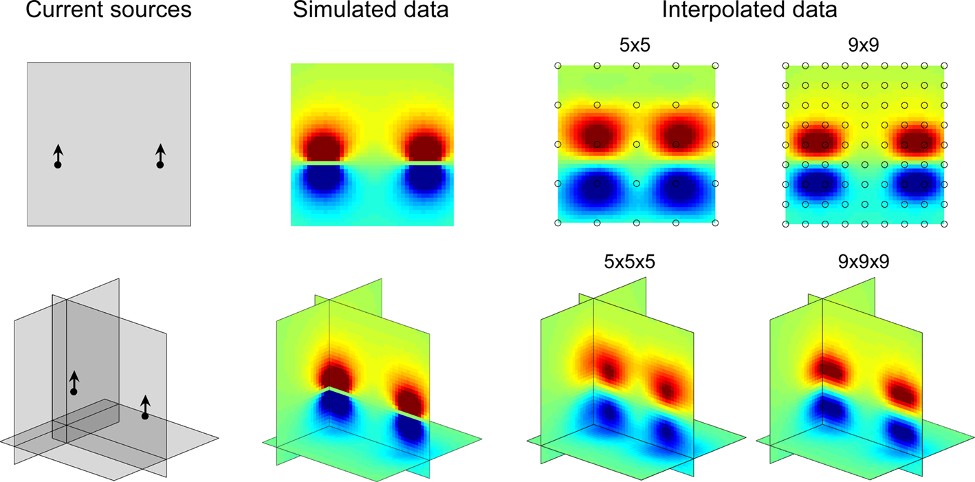
Figure 1. 2D and 3D maps of fictive MEA data. Left: current sources positions and orientations as described in Methods. Middle: simulated data computed on grids of 1681 and 68921 points for 2D and 3D configurations respectively. Right: data from fictive 5 × 5, 9 × 9, 5 × 5 × 5 and 9 × 9 × 9 MEAs interpolated on 1681 (2D) or 68921 (3D) points grids and mapped by NeuroMap. The potential field geometry can be estimated by interpolation. Note that the interpolated map is best for highest MEA resolution.

Likewise, 3D fictive sets of data were created from virtual 3D MEAs of 125 (5 × 5 × 5) or 729 (9 × 9 × 9) equally spaced electrodes, and with inter-electrode distances Δ_e and respectively. The electrode located at the center of these arrays was placed at the origin of the (x, y, z) coordinate system. The potential values were computed from the same sources (x₁ = −1.25Δ_e, y₁ = 0, z₁ = −Δ_e/2 and x₂ = 1.25Δ_e, y₂ = 0, z₂ = −Δ_e/2; see Figure 1, bottom row).

At last, a variant of the 5 × 5 × 5 data was created using potential values computed from current sources located at (x₁ = −Δ_cs/2, y₁ = 0, z₁ = 0) and (x₂ = Δ_cs/2, y₂ = 0, z₂ = 0), with Δ_cs ranging from 0 to 4Δ_e (Figure 5).

For our simulations we used Δ_e = 200 μm, but defining Δ_cs as a function of Δ_e makes our results scale-independent.

Separation Power

The possibility of improving source localization using the spatial Laplacian was investigated from the simulated data described above. The two parallel current sources create two potential fields, each one reaching its maximum amplitude in a distinct hemispace. Viewed from the recording sites, and even after careful interpolation, these two potential fields might be more or less easily differentiated, depending on the separation between the two sources (Δ_cs) in relation to the electrode pitch (Δ_e). In order to estimate the quality of this discrimination when interpolating the potential field versus interpolating the spatial Laplacian of the potential field, we define an index of separation power (SP) as follows:

where V_max is the maximum amplitude reached in each hemispace and V_mid the value at the point located between the two local maxima (see Figure 5C). The higher SP, the better the separation of the sources inferred from the interpolated map.

Image Warping

For coregistration of activity onto anatomical pictures, fine image warping is sometimes required for accurate matching of picture with recording sites locations. For this purpose, an image warping tool was implemented in NeuroMap, based on a moving least squares algorithm employing rigid transformations for a realistic deformation (Schaefer et al., 2006). This warping strategy consists in defining a set of control points p and their deformed positions q. The algorithm then constructs a deformation function f defined as f(v) = l_v(v), where l_v(x) is the best affine transformation minimizing

where p_i and q_i are coordinates of initial and deformed positions of control points respectively. The weight coefficients w_i have the form

As an affine transformation, l_v(x) can be written as l_v(x) = xM + T. Rigid transformation consists in constraining the matrix M such that M^T M = I.

This warping tool works in an interactive fashion, allowing the user to control the deformation through a set of handles that can be freely defined and positioned by mouse (see Figure 6).

The Neuromap Package

NeuroMap is licensed under GNU GPL and can be freely downloaded from a dedicated website (http://sites.google.com/site/neuromapsoftware). NeuroMap comes as a graphical user interface developed under Matlab and compatible with versions 7.1 and higher. NeuroMap has its own data format which specifies the names and 3D coordinates of the recording sites, followed by data recorded along time at each recording site. We provide NeuroMap with routines to write NeuroMap data files from Spike2 data files or Matlab variables. Besides, the distribution package includes data sets used in this paper and a comprehensive documentation.

Results

Examples of 2D and 3D maps of fictive MEA data generated by two current dipoles (see Materials and Methods) are provided in Figure 1 together with the exact calculated potential field. It appears that even with a number of electrodes as small as 25, a good approximation of the potential field pattern can be obtained using spline interpolation.

The software includes a graphical user interface (Figure 2A) allowing complete configuration of data mapping: selection of single or multiple times of mapping; selection of mapping mode (raw data, analytical, or numerical Laplacian); parameterization of the spline interpolation; loading and matching of anatomical picture with electrodes; configuration of visual rendering, including transparency effects, colormap aspect, and miscellaneous plotting-related parameters.

FIGURE 2

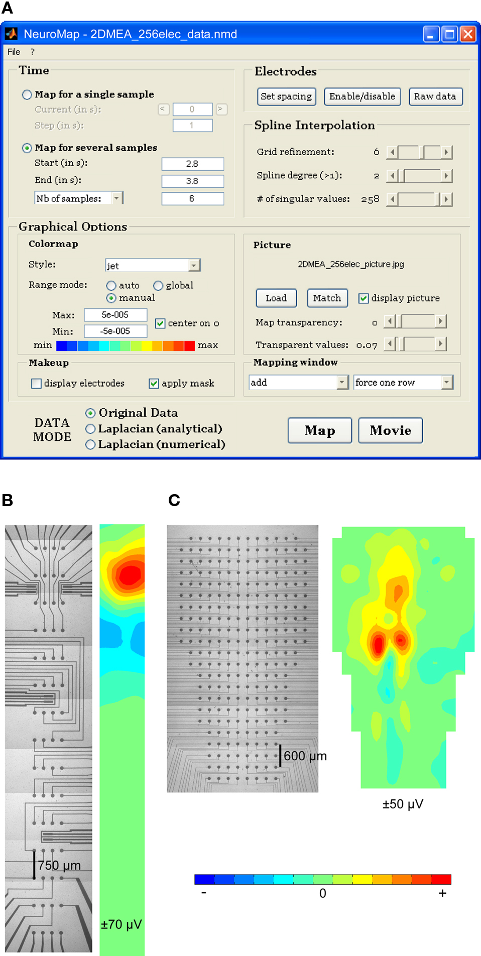
Figure 2. NeuroMap interface and mapping of experimental data from 2D MEAs. (A) NeuroMap interface for plane MEA-recorded data. (B) An example of rectangular 60-channel MEA (left) and corresponding map (right). (C) An example of irregularly shaped 256-channel MEA (left) and corresponding map (right).

Examples of 2D mapping using experimental data from a 60-electrode rectangular MEA and from a 256-electrode non-rectangular MEA are provided in Figures 2B,C, respectively.

Temporal and Spatiotemporal Representations

Due to the strong dynamic aspect of bioelectrical signals, it is essential to explore data also along the time dimension. A classical representation of both spatial and temporal features of electrical activity is time curves. NeuroMap provides such a representation, where time curves of all recording sites are positioned according to the MEA geometry (Figure 3A). It has the advantage of allowing immediate spotting of defective electrodes, which can then be disabled. Data from disabled electrodes are not used in mapping interpolation.

FIGURE 3

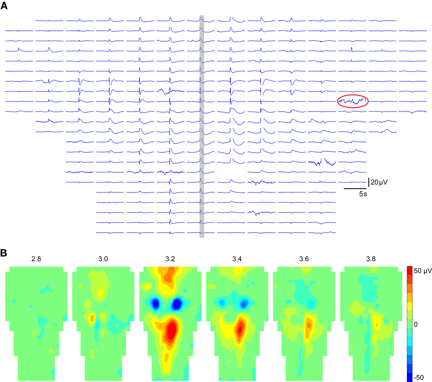
Figure 3. Temporal and spatiotemporal representations of data in NeuroMap. (A) Example of time plot in the case of 256 electrodes, positioned according to the MEA geometry. The data of the time window highlighted in gray is represented in (B) by a series of maps at regular intervals. Note that one damaged electrode (circled in A) was disabled to construct the maps. Data displayed here were obtained from the averaging of 44 individual episodes expressing the same spatiotemporal pattern.

A spatiotemporal representation of the data consists in building a series of maps at regular time intervals (Figure 3B). Such a representation is more convenient to visually detect various spatiotemporal features (initiation site, directions of propagations, etc.) than time curves.

Volume Representation of 3D Mea Data

Three-dimensional sampling of neural tissues is promising to more accurately localize activity in neural structures, as for instance to discriminate between cortical layers involved in different types of behaviors (Krupa et al., 2004). Upcoming MEA systems promise to make it a reality (Perlin and Wise, 2008; Rousseau et al., 2009). Anticipating the emergence of 3D-recording technologies, NeuroMap was designed to offer a user-friendly interface for exploration of volume data (Figure 4). All configuration possibilities offered in 2D are available in 3D, including temporal and spatiotemporal representation of data in 3D views or any x, y, or z planes in the volume of the array (not shown here).

FIGURE 4

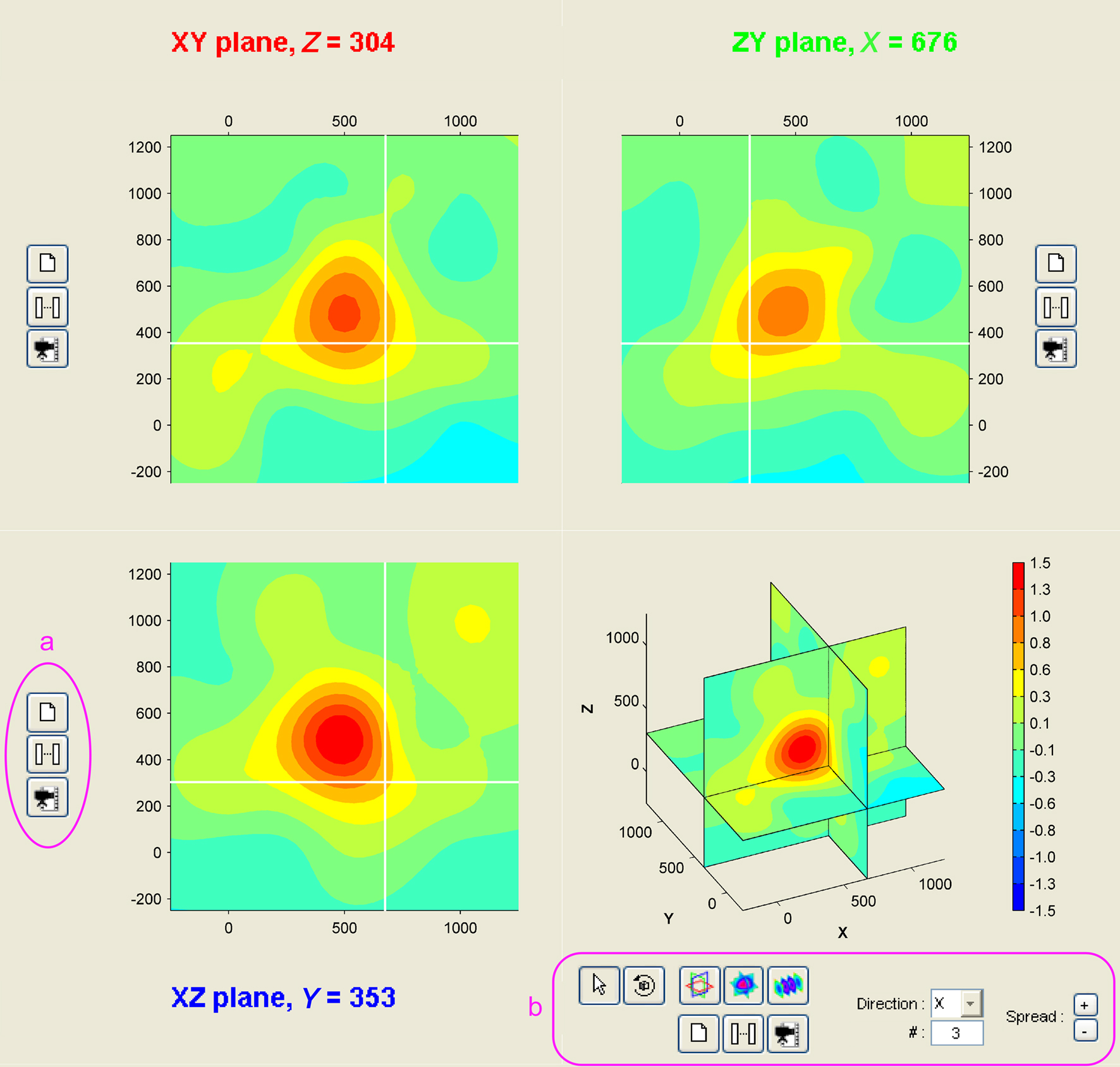
Figure 4. Volume representation of 3D MEA data. The NeuroMap interface for the exploration of 3D MEA-recorded activity presents data in three orthogonal slices: along XY (top-left), ZY (top-right), and XZ (bottom-left). White lines on each of these views indicate positions of the two other slices. User can shift these orthogonal slices in the volume by simple click on one of the three views. The interface also includes a volume view (bottom-right). To each view is associated a set of controls (a) for printing, temporal mapping, and video making. Extra controls (b) come with the volume view to modify the volume display mode: orthogonal slices (as shown here) or parallel slices; in the latter, direction and number of slices can be freely specified.

Spatial Laplacian

Spline Laplacian was shown in various human electrophysiological studies to increase significantly the spatial resolution of EEG potential distributions by providing an estimate of the cortical surface potential (Nunez and Pilgreen, 1991; Law et al., 1993; Nunez et al., 1994; Babiloni et al., 2000). In addition, providing some assumptions on the medium conductivity, one may show that the spatial Laplacian of the extracellular potential is directly linked to the current source density (Mitzdorf, 1985). Here, we implemented 2D and 3D spatial Laplacian of MEA data, which is illustrated in Figure 5 in the case of 3D simulated data (cubic 5 × 5 × 5 MEA). Raw potential and spatial Laplacian data were compared for their ability to separate the two current sources used to simulate the potential field.

FIGURE 5

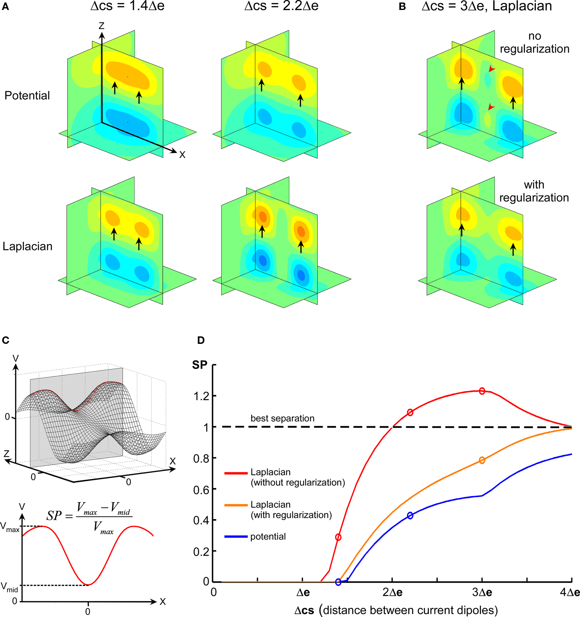
Figure 5. Comparative separation powers of raw potential and spatial Laplacian. (A) Maps illustrating the difference of separation performance between raw potential and Laplacian. (B) Top: map illustrating the phantom activity that can appear in the spatial Laplacian (red arrowheads). Bottom: phantom activity vanishes after regularization. (C) Illustration of how the SP index is calculated. In the simulated data, parallel current sources generate maximum potential field in the y = 0 plane (top). The line on which absolute maximum is reached is used. The SP index is defined using the local extrema on the maximum line (bottom). It has a value of 0 when the potential along the line has only one maximum, and is close to 1 for an optimal separation of the maxima. (D) Evolution of SP according to distance between sources (Δ_cs) for raw potential (blue), spatial Laplacian (red), and regularized Laplacian (orange). Circles indicate maps drawn in (A,B).

For distances between sources comparable to electrode pitch, the local potential extrema generated by the parallel current sources appear merged (Figure 5A, top-left), but they could be distinguished using spatial Laplacian (Figure 5A, bottom-left). When distance between sources increased, the map of raw potential could hardly display two distinct local maxima in a unique field (Figure 5A, top-right), while the Laplacian performed complete, clear-cut separation (Figure 5A, bottom-right). For large distances between sources, the spline Laplacian tended to generate phantom activity between the two fields (Figure 5B, top) due to rebounds of the spline, a phenomenon that could be corrected by regularization (Figure 5B, bottom; see Resolution and Regularization in Materials and Methods).

The performance of source separation was further investigated systematically for intersource distance Δ_cs ranging from 0 to 4 Δ_e by 0.05 × Δ_e steps. Figure 5C illustrates how the SP index was calculated (see also Materials and Methods). Figure 5D displays SP values in the whole Δ_cs range for potential and Laplacian interpolations. Spatial Laplacian always improved sources separation when compared to raw potential. While regularized Laplacian displayed a lower SP than original Laplacian, it remained more effective than raw potential for source separation.

Coregistration on Anatomical Images

A major feature of the MEA technology is the possibility to cover a large network and to study interactions between various areas. For this purpose, it can be useful to merge signal data with anatomical data. NeuroMap offers a convenient way to do so by coregistration of maps of activity onto images, which are typically pictures of the recorded preparation (Figure 6A1). To perform this coregistration, the software requires only information about the exact localization of the electrodes on the picture. This is determined from the positions of two reference electrodes, selected and indicated on the picture by the user (Figures 6A2,A3).

FIGURE 6

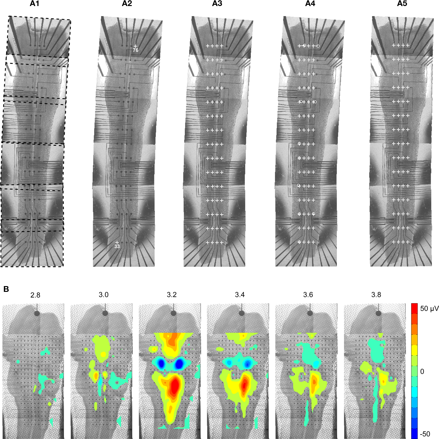
Figure 6. Coregistration of activity data onto anatomical picture. (A1) The picture of a whole embryonic hindbrain–spinal cord preparation recorded with a 4 ×] 15 MEA was rebuilt from six partial pictures (dashed frames). As partial pictures have not been perfectly aligned during reconstruction, the anatomical picture needs appropriate warping to match the real MEA geometry. (A2) First, user identifies two or more electrodes on the picture (white crosses). (A3) Using the identified electrodes coordinates, the program computes the scale of the picture and the theoretical positions of all electrodes (white crosses). As expected, these do not match the electrodes of the picture. (A4) In order to perform appropriate deformation of the picture, the user specifies the correspondence between theoretical and pictured positions for a few electrodes (white circles). These landmarks determine reference pixel displacements that are extrapolated for the whole image. (A5) Result after application of the deformation algorithm. (B) Mapping of activity on a matched anatomical picture of an embryonic hindbrain (data is identical to that of Figure 3B). In order to improve visibility of the anatomy, values in the noise range (±4 μV) were not displayed.

When large structures are considered, the full image is usually obtained by stitching several smaller fields of views, a process that may introduce distortions in the final anatomical image reconstruction. In order to compensate for these distortions and achieve accurate registration of data mapping on the anatomy of the tissue, image warping can be performed (Figures 6A4,A5).

Matching electrode locations onto anatomical picture is possible for any geometry of MEA. An example of 256-channel activity coregistered onto the anatomy of an embryonic mouse hindbrain is shown in Figure 6B. The visual rendering of coregistration can be further improved by applying transparency to activity data (not shown here), or by thresholding mapped values so as to emphasize regions of highest activity, as in Figure 6B.

Discussion

We presented NeuroMap, an interactive software for spatiotemporal mapping of 2D and 3D MEA data.

NeuroMap can be fed with any quantity at each electrode, which can be either raw bioelectric data or processed data derived from recordings (e.g., spike firing rates, LFPs, etc.). To build maps, NeuroMap estimates data between recording sites using thin plate spline interpolation. This method provides a smooth estimation of data and can predict the presence of extrema between the electrodes, unlike nearest-neighbor or bilinear interpolation approaches. The use of this software is not restricted to classical rectangular and planar commercial systems, nor to a regular spacing between electrodes. NeuroMap was designed to deal with any geometry of arrays, so as to handle the whole variety of MEA layouts that may be developed for specific uses or neural structures (e.g., hippocampus, brainstem, etc.). It is as well adapted to those forthcoming 3D arrays that will provide recording sites in all directions of space.

Spatial Laplacian is an effective approach to further increase spatial resolution and accurately estimate the locations of the current sources that underlie the observed extracellular potential field. NeuroMap takes the whole advantage of the analytical formulation of splines to build spatiotemporal representations of the spatial Laplacian. It should be noted that the estimation of spatial Laplacian is not possible using bilinear nor nearest-neighbor interpolation approaches, which provide zero or ill-defined second derivatives. This could be overcome by the use of higher order polynomial approaches such as Bezier which are less computationally time consuming than thin plate splines. However, such approach would fail in the case of irregular electrode spacing or when some non-functional electrodes of the array are discarded for mapping.

The potentiality of high spatial resolution is further exploited with coregistration of activity data onto anatomical pictures. Used with data from high-density arrays that cover macroscopic neural networks, NeuroMap can provide exhaustive mapping of whole structures. This approach opens interesting possibilities for more thorough physiological interpretation of MEA recordings, with, for instance, the merging of activity data with subsequent immunohistochemical labeling.

In conclusion, NeuroMap provides an open-source tool to visualize spatiotemporal MEA data, which can further help in the identification and segregation of multiple activity patterns over the detailed anatomy of large neural structures.

Conflict of Interest Statement

The authors declare that the research was conducted in the absence of any commercial or financial relationships that could be construed as a potential conflict of interest.

Acknowledgments

This work was supported in part by the French National Research Agency (ANR) Programme Blanc No. ANR06BLAN035601 and Programme TecSan No. ANR-08-TECS-018-05. The authors also wish to thank Lionel Rousseau (ESIEE-Paris) for making the 256 channel MEAs and Guillaume Charvet, Olivier Billoint, Sadok Gharbi, and Régis Guillemaud from CEA-LETI for their contribution to the development of the BioMEA system used here.

References

Babiloni, F., Babiloni, C., Carducci, F., Fattorini, L., Onorati, P., and Urbano, A. (1996). Spline Laplacian estimate of EEG potentials over a realistic magnetic resonance-constructed scalp surface model. Electroencephalogr. Clin. Neurophysiol. 98, 363–373.

Pubmed Abstract | Pubmed Full Text

Babiloni, F., Babiloni, C., Locche, L., Cincotti, F., Rossini, P. M., and Carducci, F., (2000). High-resolution electro-encephalogram: source estimates of Laplacian-transformed somatosensory-evoked potentials using a realistic subject head model constructed from magnetic resonance images. Med. Biol. Eng. Comput. 38, 512–519.

Pubmed Abstract | Pubmed Full Text | CrossRef Full Text

Beggs, J. M., and Plenz, D. (2003). Neuronal avalanches in neocortical circuits. J. Neurosci. 23, 11167–11177.

Pubmed Abstract | Pubmed Full Text

Berdondini, L., van der Wal, P. D., Guenat, O., de Rooij, N. F., Koudelka-Hep, M., Seitz, P., Kaufmann, R., Metzler, P., Blanc, N., and Rohr, S. (2005). High-density electrode array for imaging in vitro electrophysiological activity. Biosens. Bioelectron. 21, 167–174.

Pubmed Abstract | Pubmed Full Text | CrossRef Full Text

Charvet, G., Rousseau, L., Billoint, O., Gharbi, S., Rostaing, J. P., Joucla, S., Trevisiol, M., Bourgerette, A., Chauvet, P., Moulin, C., Goy, F., Mercier, B., Colin, M., Spirkovitch, S., Fanet, H., Meyrand, P., Guillemaud, R., and Yvert, B. (2010). BioMEA (TM): a versatile high-density 3D microelectrode array system using integrated electronics. Biosens. Bioelectron. 25, 1889–1896.

Pubmed Abstract | Pubmed Full Text | CrossRef Full Text

Csicsvari, J., Henze, D. A., Jamieson, B., Harris, K. D., Sirota, A., Bartho, P., Wise, K. D., and Buzsaki, G. (2003). Massively parallel recording of unit and local field potentials with silicon-based electrodes. J. Neurophysiol. 90, 1314–1323.

Pubmed Abstract | Pubmed Full Text | CrossRef Full Text

Duchon, J. (1976). Interpolation of 2-variable functions following principle of thin plate flexion. Revue Française D’Automatique Informatique Recherche Operationnelle 10, 5–12.

Harder, R. L., and Desmarais, R. N. (1972). Interpolation using surface splines. J. Aircr. 9, 189–191.

CrossRef Full Text

Joucla, S., and Yvert, B. (2009). Improved focalization of electrical microstimulation using microelectrode arrays: a modeling study. PLoS ONE 4, e4828. doi: 10.1371/journal.pone.0004828

Pubmed Abstract | Pubmed Full Text | CrossRef Full Text

Krupa, D. J., Wiest, M. C., Shuler, M. G., Laubach, M., and Nicolelis, M. A. L. (2004). Layer-specific somatosensory cortical activation during active tactile discrimination. Science 304, 1989–1992.

Pubmed Abstract | Pubmed Full Text | CrossRef Full Text

Law, S. K., Rohrbaugh, J. W., Adams, C. M., and Eckardt, M. J. (1993). Improving spatial and temporal resolution in evoked EEG responses using surface Laplacians. Electroencephalogr. Clin. Neurophysiol. 88, 309–322.

Pubmed Abstract | Pubmed Full Text

Malmivuo, J., and Plonsey, R. (1995). Bioelectromagnetism. New York: Oxford University Press.

Mitzdorf, U. (1985). Current source-density method and application in cat cerebral-cortex – investigation of evoked-potentials and EEG phenomena. Physiol. Rev. 65, 37–100.

Pubmed Abstract | Pubmed Full Text

Nicolelis, M. A. L., Ghazanfar, A. A., Faggin, B. M., Votaw, S., and Oliveira, L. M. O. (1997). Reconstructing the engram: simultaneous, multisite, many single neuron recordings. Neuron 18, 529–537.

Pubmed Abstract | Pubmed Full Text | CrossRef Full Text

Nunez, P. L., and Pilgreen, K. L. (1991). The spline-Laplacian in clinical neurophysiology – a method to improve EEG spatial-resolution. J. Clin. Neurophysiol. 8, 397–413.

Pubmed Abstract | Pubmed Full Text | CrossRef Full Text

Nunez, P. L., Silberstein, R. B., Cadusch, P. J., Wijesinghe, R. S., Westdorp, A. F., and Srinivasan, R. (1994). A theoretical and experimental-study of high-resolution EEG based on surface Laplacians and cortical imaging. Electroencephalogr. Clin. Neurophysiol. 90, 40–57.

Pubmed Abstract | Pubmed Full Text

Perlin, G. E., and Wise, K. D. (2008). “A compact architecture for three-dimensional neural microelectrode arrays,” in 30th Annual International Conference of the IEEE Engineering in Medicine and Biology Society, Vols 1–8 (New York: IEEE), 5806–5809.

Perrin, F., Pernier, J., Bertrand, O., Giard, M. H., and Echallier, J. F. (1987). Mapping of scalp potentials by surface spline interpolation. Electroencephalogr. Clin. Neurophysiol. 66, 75–81.

Pubmed Abstract | Pubmed Full Text

Rolston, J. D., Wagenaar, D. A., and Potter, S. M. (2007). Precisely timed spatiotemporal patterns of neural activity in dissociated cortical cultures. Neuroscience 148, 294–303.

Pubmed Abstract | Pubmed Full Text | CrossRef Full Text

Rousseau, L., Verjus, F., Rouessard, J., Abdoun, O., Mazzocco, C., Lissorgues, G., and Yvert, B. (2009). “Design of new microelectrode arrays for a 3D sampling of the neural tissue,” in Society for Neuroscience Abstract 586.19, Chicago.

Schaefer, S., McPhail, T., and Warren, J. (2006). Image deformation using moving least squares. ACM Trans. Graph. 25, 533–540.

Shahaf, G., and Marom, S. (2001). Learning in networks of cortical neurons. J. Neurosci. 21, 8782–8788.

Pubmed Abstract | Pubmed Full Text

Steidl, E. M., Neueu, E., Bertrand, D., and Buisson, B. (2006). The adult rat hippocampal slice revisited with multi-electrode arrays. Brain Res. 1096, 70–84.

Pubmed Abstract | Pubmed Full Text | CrossRef Full Text

Tscherter, A., Heuschkel, M. O., Renaud, P., and Streit, J. (2001). Spatiotemporal characterization of rhythmic activity in rat spinal cord slice cultures. Eur. J. Neurosci. 14, 179–190.

Pubmed Abstract | Pubmed Full Text

Uutela, K., Hamalainen, M., and Somersalo, E. (1999). Visualization of magnetoencephalographic data using minimum current estimates. Neuroimage 10, 173–180.

Pubmed Abstract | Pubmed Full Text | CrossRef Full Text

Wagenaar, D. A., Madhavan, R., Pine, J., and Potter, S. M. (2005). Controlling bursting in cortical cultures with closed-loop multi-electrode stimulation. J. Neurosci. 25, 680–688.

Pubmed Abstract | Pubmed Full Text | CrossRef Full Text

Yvert, B., Crouzeix-Cheylus, A., and Pernier, J. (2001). Fast realistic modeling in bioelectromagnetism using lead-field interpolation. Hum. Brain Mapp. 14, 48–63.

Pubmed Abstract | Pubmed Full Text | CrossRef Full Text