An efficient simulation environment for modeling large-scale cortical processing
- 1 Department of Cognitive Sciences, University of California, Irvine, CA, USA
- 2 Department of Computer Science, University of California, Irvine, CA, USA
We have developed a spiking neural network simulator, which is both easy to use and computationally efficient, for the generation of large-scale computational neuroscience models. The simulator implements current or conductance based Izhikevich neuron networks, having spike-timing dependent plasticity and short-term plasticity. It uses a standard network construction interface. The simulator allows for execution on either GPUs or CPUs. The simulator, which is written in C/C++, allows for both fine grain and coarse grain specificity of a host of parameters. We demonstrate the ease of use and computational efficiency of this model by implementing a large-scale model of cortical areas V1, V4, and area MT. The complete model, which has 138,240 neurons and approximately 30 million synapses, runs in real-time on an off-the-shelf GPU. The simulator source code, as well as the source code for the cortical model examples is publicly available.
Introduction
The mammalian nervous system is a network of extreme size and complexity (Sporns, 2011), and understanding the principles of brain processing by reverse engineering neural circuits and computational modeling is one of the biggest challenges of the Twenty-first century (Nageswaran et al., 2010), see also (National Academy of Engineering-Grand Challenges for Engineering1). Thus, there is a need within the computational neuroscience community for simulation environments that can support modeling at a large-scale, that is, networks which approach the size of biological nervous systems. In particular, we consider large-scale network models of spiking neurons. Spiking models can demonstrate temporal dynamics, precise timing, and rhythms that are important aspects of the neurobiological processing of information (Vogels et al., 2005). Moreover, spiking models, with their digital signaling and sparse coding, are energy efficient and amenable to hardware application development (Mead, 1990; Laughlin and Sejnowski, 2003).
There are several spiking simulators, which are currently available, that fall into different categories based on their level of abstraction and on the computer hardware in which they reside (for a recent review see Brette et al., 2007). Simulators, such as GENESIS and NEURON, incorporate molecular, detailed compartmental models of axons and dendrites from anatomical observations, and various ion channels to biophysical details (Hines and Carnevale, 1997, 2001; Bower and Beeman, 2007). A major goal of these models is to study detailed ionic channels and their influence on neuronal firing behavior. While these models are biologically accurate, they incur tremendous computational costs for simulation. Typically, these neuronal models are multi-compartmental to take into consideration dendritic morphology and distribution of ionic currents across the neuron. All of these components are modeled with differential equations having time steps less than 1 ms. Hence, large-scale simulation of the brain is extremely challenging at this level.
Neuromorphic designs, such as NEUROGRID, and SPINNAKER, are efficient enough to run large-scale networks of spiking neurons, but require specialized hardware (Boahen, 2005, 2006; Navaridas et al., 2009; Rangan et al., 2010). Therefore, these systems are not readily available to the computational neuroscience community.
Simulation environments, such as the neo cortical simulator (NCS; Drewes et al., 2009; Jayet Bray et al., 2010), Brian (Goodman and Brette, 2008, 2009), Neural Simulation Tool (NEST; Gewaltig and Diesmann, 2007), and NeMo (Fidjeland and Shanahan, 2010) are specifically designed for developing spiking neuron networks. However, each simulator environment has different tradeoffs in speed, realism, flexibility, maximum network size, etc. For example Brian is extremely flexible but incurs a performance penalty for that flexibility. NCS is powerful and can run on computer clusters, but does not incorporate a standard interface.
Our approach is to design a simulator that is easy to use and yet provide significant computational performance. We achieve this by using a PyNN-like interface and abstraction (Davison et al., 2008). PyNN is a common programming interface developed by the neuronal simulation community to allow a single script to run on various simulators. Although our simulator is not compliant with the PyNN API, we chose a similar interface since it is easy to use, and will be familiar to many users. For the neuron model, we use the Izhikevich neuron model, which is an efficient model that supports a wide-range of biophysical dynamics, but has very few open parameters (Izhikevich, 2004). To model synaptic plasticity, we use standard equations for spike-timing dependent plasticity (STDP; Song et al., 2000) and short-term plasticity (STP; Markram et al., 1998; Mongillo et al., 2008). Finally, to ensure our simulator can be supported on a wide-range of machines, our simulator runs on both generic x86 CPUs and NVIDIA GPUs under Windows and Unix operating systems.
In prior work, we developed and released a GPU implementation of current-based spiking neural networks (SNN) that was 26 times faster than a CPU version (Nageswaran et al., 2009). For simulations of 10 million synaptic connections and 100 K neurons, the GPU SNN model was only 1.5 times slower than real-time. That is, the time to calculate 1 ms of time in the differential equations describing the neurons and synapses was equivalent to 1.5 ms of wall clock time. In this prior work, we introduced optimization techniques for parallelism extraction, mapping of irregular communication, and network representation for effective simulation of SNNs on GPUs. Comparing responses against a CPU version validated the computational fidelity of the GPU simulation, and comparing the simulated neuronal firing rate, synaptic weight distribution, and inter-spike interval with electrophysiological data validated the neurobiological fidelity. We made the simulator publicly available to the modeling community so that researchers would have easy access to large-scale SNN simulations. There have been other recent, notable spiking simulators, which use GPUs to accelerate computation (Fidjeland and Shanahan, 2010; Yudanov et al., 2010). However, NeMo, Yudanov et al. (2010), and our previous simulator had shortcomings, with respect to synaptic dynamics, that limited the biological accuracy of network simulations.
Therefore, in the present paper, we extend our prior model to include: (1) a better, more flexible interface for creating neural networks, (2) equations for AMPA, GABA, and NMDA conductance (Izhikevich et al., 2004), (3) equations for STP (Markram et al., 1998; Mongillo et al., 2008), and (4) an efficient implementation of a motion energy model for generating motion selective responses (Simoncelli and Heeger, 1998). As in our prior work, the goal is to make large-scale, efficient SNN simulations readily available to a wide-range of researchers. Although the SNN simulator is written in C++, only some familiarity with C/C++ is necessary to use our simulator. We illustrate the power and ease of use of the simulation environment with several examples below.
The present simulation environment, which incorporates optimizations used in our prior work and optimizations for the new functionality, allows for efficient implementation of large-scale SNNs. GPU execution times can be faster than real-time for even moderate to large-scale networks (on the order of 100,000 neurons with 1,000 synapses each). In one of examples below, we introduce a network with 138,000 neurons and 30 million synapses that runs in real-time.
In the sections below, we will highlight the benefits of our simulator as well as provide an outline for how custom models can be implemented in the simulator. Table 1 lists the complete functionality of the simulation environment. We will provide examples for some of the more commonly used functions and options. Specifically, we will discuss how to define groups and connections, how to specify inputs to and get outputs from the networks, and how to store the network state.
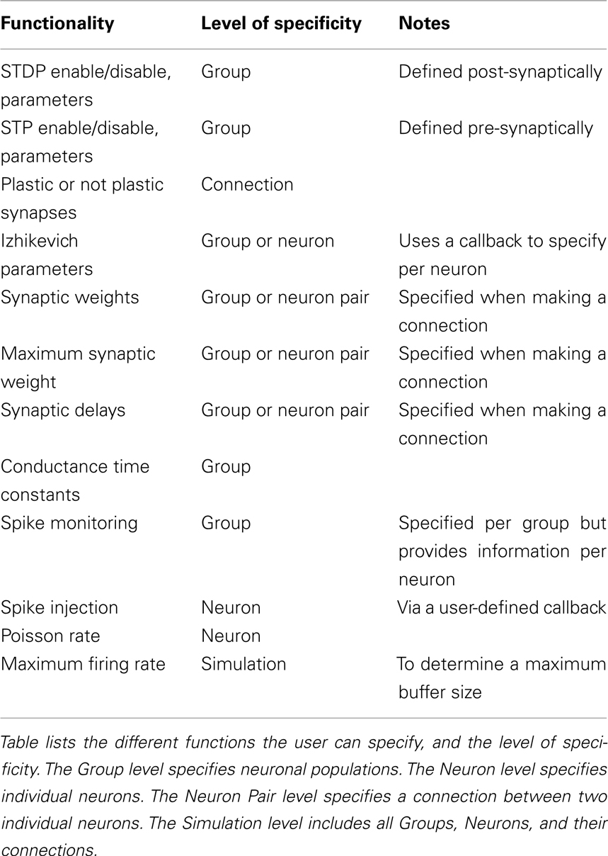
Table 1. Functionality of the simulation environment.
In the last section, we describe a large-scale model of cortical areas V1, V4, and MT, developed with our simulator, that demonstrates its ease of use, and computational power. Further, using these medium level visual processing simulations may benefit other researchers in their model development.
The source code for the simulator, networks, and analysis scripts can be obtained in the supplemental file: “http://www.socsci.uci.edu/∼jkrichma/Richert-FrontNeuroinf-SourceCode.zip.” The main code to run the examples described below can be found in the “examples” directory and MATLAB scripts to analyze the simulation results can be found in the “scripts” directory within the supplemental source code directory. MATLAB is not necessary to use the simulator. In general, any program can be used to analyze the simulation results. The MATLAB scripts are provided for demonstration purposes and can easily be translated to the user’s preferred analysis tool.
Materials and Methods
Model Capabilities
Our simulator was first published in (Nageswaran et al., 2009), but has been greatly enhanced to improve functionality and ease of use. The present simulator uses the four parameter Izhikevich point-neurons (see Eq. 1) and all four parameters can be specified per neuron or per group. The simulator supports synaptic currents or conductances. Currently, four conductances are supported: AMPA (fast decay), NMDA (slow decay and voltage dependent), GABAA (fast decay), GABAB (slow decay). All time constants are configurable. The model also supports standard implementations of the nearest neighbor formulation of STDP [see Eq. 2, (Song et al., 2000)] and STP [see Eq. 3, (Markram et al., 1998; Mongillo et al., 2008)].
The Izhikevich neuron is a dynamical systems model that can be described by the following update equations:
If v=30 mV then v=c, u = u + d
Where, v is voltage, u is the recovery variable, I is the input current, and a, b, c, d are open parameters that have different values for different neuron types.
Spike-timing dependent plasticity is a biological synaptic plasticity rule that takes into consideration the relative timing of pre- and post-synaptic spikes:
Where A+ and A− determine the height of the STDP curves, and τ+, τ− are time constants, and Δt is the time of the post-synaptic spike minus the time of the pre-synaptic spike.
Short-term plasticity is a faster scale synaptic plasticity rule, on the order of 100 ms, that contributes to synaptic facilitation and synaptic depression and is based on pre-synaptic activity:
Where δ is the Dirac function, tspk is the time of the pre-synaptic spike, x and u recover to their baseline levels (x = 1 and u = U) with time constants tD (depressing) and tF (facilitating), respectively, and st is the STP scale factor applied to the synaptic weight at time t.
Table 1 lists the functionality of the simulator. Functionality can be enabled or disabled, such as one group of neurons can have STDP while another group in the same simulation does not have STDP. Most operations are specified at the Group (i.e., neuronal population) level. Many options can be specified at the level of Neuron but to have that level of control the user must create a callback mechanism as described below.
Calculations in the simulation used the forward Euler method with dt = 1 ms for synaptic plasticity equations and dt = 0.5 ms for the neuronal activity equations.
Building and Running a Simulation
In the following sections, we outline step-by-step instructions on how to set up, construct, and execute a simulation.
Setting up a simulation
To begin a simulation, the user must import the simulator and create an instance:
         #include “snn.h”

…

CpuSNN sim(“My Simulation”);
Similar to PyNN and many other simulators, our simulator uses groups and connections as an abstraction to aid defining synaptic connectivity.
A group is composed of one or more neurons and is used for organizational convenience. Two types of groups are supported: Izhikevich neurons and spike generators. Spike generators are pseudo-neurons that have their spikes specified externally either defined by a Poisson firing rate or via a spike injection mechanism. Spike generators can have post-synaptic connections with STDP and STP, but unlike Izhikevich neurons, they do not receive any pre-synaptic inputs. Spike generators can be used to convert inputs, such as an image, into spike trains.
To create a group of Izhikevich neurons, simply specify a name (e.g., “excitatory”), the number of neurons (e.g., 100), and a type:
         int gEx=sim.createGroup(“excitatory”, 100,
EXCITATORY_NEURON);
Where EXCITATORY_NEURON denotes that the neurons in this group are glutamatergic and the group ID (used to refer to this group for later method calls) is returned and stored in the variable gEx. The name can be anything and is written to the network data file (see section Storing and retrieving the network state) to make it easier for the user to identify groups.
Next, specify the Izhikevich parameters:
sim.setNeuronParameters(gEx, 0.02f, 0.2f,
-65.0f, 8.0f);
Where 0.02f, 0.2f, −65.0f, and 8.0f correspond respectively to the a, b, c, and d parameters of the Izhikevich neuron.
To create a group of spike generators, the user also specifies a name, size, and type:
int gIn=sim.createSpikeGeneratorGroup(“input”, 10, EXCITATORY_NEURON);
Where gIn is group ID, “input” is the name of the group, 10 is the number of neurons, and EXCITATORY_NEURON denotes that the neurons in this group are glutamatergic.
To implement groups of neurons in CUDA, the groups were reordered such that groups and neurons of similar types are localized, however, only one kernel is used. The kernel looks up the group identity of each neuron, as well as other information specific to each neuron.
Making connections
Pre-defined connection types. Once the neuron groups have been defined, the synaptic connections between them can be defined. The simulator provides a set of primitive connection topologies for building networks: (1) All-to-all, (2) One-to-one, and (3) Random. All-to-all, also known as “full,” connectivity specifies that all neurons in the pre-synaptic group should be connected to all neurons in the post-synaptic group. One-to-one connectivity denotes when neuron i in the pre-synaptic group is connected to neuron j in the post-synaptic group; both pre- and post-synaptic groups should have the same number of neurons. Random connectivity denotes when a group of pre-synaptic neurons are randomly connected to a group of post-synaptic neurons with a probability p; where the user specifies p. For all pre-defined connection types the user specifies an initial synaptic weight, a maximum synaptic weight, and a range of synaptic delays.
Creating connections with the pre-defined types is quite simple. The following statement creates a random connection pattern from group gIn to group gEx with an initial weight of 1.0, a maximum weight of 1.0, a 10% (0.10) probability of connection, a synaptic delay uniformly distributed between 1 and 20 ms, and static synapses (SYN_FIXED):
sim.connect(gIn, gEx,“random”, 1.0, 1.0,

0.10f, 1, 20, SYN_FIXED);
User-defined connections. The pre-defined topologies described above are useful for many simulations, but are insufficient for constructing networks with realistic neuroanatomy. In order to provide arbitrary and flexible connectivity, we introduce a callback mechanism. In the callback mechanism, the simulator calls a method on a user-defined class in order to determine whether a connection should be made or not. The user simply needs to define a method that specifies whether a connection should be made between a pre-synaptic neuron and a post-synaptic neuron and the simulator will automatically call the method for all possible pre-, and post-synaptic pairs. The user can then specify the connection’s delay, initial weight, maximum weight, and whether or not it is plastic.
To make a user-defined connection, the user starts by making a new class that derives from the Connection Generator class:
class MyConnection: public


ConnectionGenerator { …
Inside this new class, the user defines a connect method. The following statements show a simple example that creates random connections with a 10% probability:
         void connect(CpuSNN* net,

int srcGrp, int src, int destGrp, int dest,

                               float& weight, float& maxWt,

float& delay, bool& connected)

{

      connected = getRand()<0.10;

      weight = 1.0;

      maxWt = 1.0;

      delay = 1;

}
Once the class has been defined, simply call connect on the simulator as follows:
sim.connect(gIn, gEx, new MyConnection(),

SYN_PLASTIC);
Running a simulation
Once a network has been specified running the network is quite simple. The user need only call:
sim.runNetwork(sec, msec, mode);
Where the simulation will run for sec*1000 + msec milliseconds and mode can be either CPU_MODE or GPU_MODE to specify which hardware to run the simulation on: CPU or GPU.
Interacting with the Simulation
To interact with the simulation, the user defines spike generators for injecting inputs and spike monitors for retrieving outputs. The simulator provides a simple mechanism to define Poisson firing rates, and an easy-to-use mechanism to define spike times via a user-defined callback. To retrieve outputs, a spike-monitoring callback mechanism is used. The user registers a custom method and then the spike monitor, which is automatically called once a second, specifies the neuron and the time it fired during the last second.
Generator groups
There are two types of input groups supported and both are called spike generators. The first group type is the Poisson Generators, which generates Poisson spike trains based upon a specified average firing rate. The second group type is the Spike Injection Generators, in which spike times are specified via a user-defined callback.
Poisson generators. The simulator supports specifying the mean firing rate for each neuron within a generator group. Furthermore, the rates can be changed at every time step (1 ms) for extremely fast input modulation.
To make a Poisson generator, the user first specifies the firing rates for each neuron by creating a Poisson Rate object of the same size as the Poisson group, and then fills in the values for each neuron:
PoissonRate ramp(10);

for (int i=0;i<10;i++) ramp.rates[i] = 1+i;
Once the firing rates have been specified simply call setSpikeRate:
sim.setSpikeRate(gIn,&ramp);
Spike injection generators. For more fine-grained control over spike generation, individual spike times can be specified per neuron in each group. This is accomplished by using a callback mechanism, which is called at each time step, to specify whether a neuron has fired or not.
In order to specify spike times, a new class is defined that derives from the Spike Generator class:
class MySpikes: public SpikeGenerator { …
The user must then define a nextSpikeTime method. The following is a simple example that generates a spike every 100 ms for each neuron in the group.
         unsigned int nextSpikeTime(CpuSNN* s,

int grpId, int nid, unsigned int

currentTime)

{

      return currentTime + 100;

}

…

sim.setSpikeGenerator(gIn,new MySpikes());
Spike monitoring
In order to calculate basic statistics, store spike trains, or perform more complicated output monitoring, the user can specify a spike monitor. Spike monitors are registered for a group and are called automatically by the simulator every second. Similar to an address event representation (AER), the spike monitor indicates which neurons spiked by using the neuron ID within a group (0 is the first neuron in a group) and the time of the spike. Only one spike monitor is allowed per group. Therefore, if the user desires having multiple monitors running on a single group, the user must call additional monitors from within their own spike monitor.
There are several options for spike monitoring. The following code will print basic information to the screen about the group’s activity, such as the average firing rate and current time of the simulation:
s.setSpikeMonitor(gIn);
Instead of printing basic information to the screen, the following code creates a file that stores all spikes generated by the group:
s.setSpikeMonitor(gIn,“spikes.dat”);
The file format is simply a list of Neuron ID and spike time (in ms) pairs, each stored as unsigned 32 bit integers. In general, any programming language can be used to read and analyze these files. In Section “A MATLAB Function to Read the Spike Data Files” in Appendix, we present an example, using MATLAB code, of how these spike data files can be read.
A user can create custom spike monitors by creating a new class that derives from Spike Monitor and by defining an update method. For example, the following statements show a custom spike monitor that prints a message when neuron 50 fires:
         class MyMonitor: public SpikeMonitor {…

void update(CpuSNN* s, int grpId,

unsigned int*NeuronIds, unsigned int*

timeCounts)

{

   int pos = 0;

 for (int t=0; t < 1000; t++) {

      for(int i=0; i < timeCounts [t];i++,
pos++) {

         int id = NeuronIds [pos];

         if (id == 50) cout << “Neuron

ID 50 spiked at” << t >> “ms.\n”;

      }

   }

}
The update method is passed two arrays: NeuronIds and timeCounts. NeuronIds stores a list of Neuron IDs within a group which have spiked. TimeCounts is an array of length 1000, which corresponds to 1000 ms. TimeCounts [0] indicates how many neurons spiked in the first time bin (0 ms) and timeCounts [1] for the second time bin (1 ms), etc., up to timeCounts [999] which is for 999 ms. So, if there have not been any spikes in the past 1000 ms, the array timeCounts would contain all zeros.
The example code above works by using a variable “pos” which stores the current position into the NeuronIds array and looping through all 1000 time bins. The inner for-loop then loops through the number of neurons that spiked in time bin “t” and increments “pos” simultaneously. Then the neuronID can be extracted at position “pos” and stored in variable “id.” In the example above, if a neuron with the id of 50 fires, then an output message is generated indicating when it spiked within this 1000 ms block.
Storing and Retrieving the Network State
Once all connections have been specified and the network has been instantiated, the network state can be stored in a file for later processing or for restoring a specific network. The network state consists of all the synaptic connections, weights, delays, and whether the connections are plastic or fixed. Furthermore, the network can be stored after synaptic learning has occurred in order to externally analyze the learned synaptic patterns.
The following code stores a network:
FILE* nid = fopen(“network.dat”,“wb”);

sim.writeNetwork(nid);

fclose(nid);
After a network has been stored, following code will reload the network:
FILE* nid = fopen(“network.dat”,“rb”);

sim.readNetwork(nid);

//don’t fclose nid here, call

         sim.runNetwork() first
The network file can be read by the MATLAB code shown in Section “A MATLAB Function to Read the Stored Network Files” in Appendix.
However, writing the network state to file is not the only method provided to access this information; one can retrieve the weight and delay information for a specific neuron by calling getWeights() or getDelays() respectively. For example, the following code will output the weight value of a particular synapse:
         int Npre, Npost;

float* weights = sim.getWeights(gIdPre,

gIdPost, Npre, Npost);

cout << “The weight of the synapse between

         presynaptic neuron 3 and

postsynaptic neuron 5 is<< weights[5+Npre*3]<< endl;
GPU vs. CPU Simulation Modes
One of the main features of the simulator, beyond its ease of use, is the computational efficiency of the code base. The simulator has been implemented to be able to run on either standard x86 CPUs or off-the-shelf NVIDIA GPUs. Aside from specifying which architecture to run the simulator on (sim.runNetwork(…,CPU_MODE) vs. sim.runNetwork(…,GPU_MODE)), there are no code modifications required from the user.
The ability to run on either architecture allows the user to exploit the advantages of both. The CPU is more efficient for small networks, or allows for running extremely large networks that do not fit within the GPU’s memory. The GPU is most advantageous for large networks (1 K to approximately 100 K neurons) and has been demonstrated on our hardware (Core i7 920 @2.67 GHz and NVIDIA C1060) to run up to 26 times faster than CPU and allow for approximately real-time performance for a simulation of 100 K neurons (Nageswaran et al., 2009).
Results
In the following sections we provide several complete examples of the SNN developed with our simulation environment. We demonstrate a complete Spiking Neural Network that demonstrates typical spike dynamics found in random networks having the appropriate balance of excitatory and inhibitory neurons, and STDP. We also describe the construction of a large-scale network for cortical visual processing. The network includes cortical areas V1, V4, and MT. We demonstrate that the color, orientation, and motion selectivity of neurons in the network are comparable to electrophysiological and biophysical data.
The source code to run all the simulations described below can be obtained at: http://www.socsci.uci.edu/∼jkrichma/Richert-FrontNeuroinf-SourceCode.zip.
A Complete Example
In Section “Simple Source Code to Make a Randomly Connected Network Capable of Sustained Activity and Learning” in the Appendix contains example source code of a randomly connected network with STDP. The network contains 1,100 neurons and approximately 68,000 excitatory synapses and approximately 16,000 inhibitory synapses. The conductances of the model and STDP parameters are set to physiologically realistic values and are taken from (Izhikevich, 2006). The network is a simple 80/20 network (i.e., 80% excitatory and 20% inhibitory neurons) that has been used to generate random asynchronous intermittent neural (RAIN) activity (Vogels and Abbott, 2005; Vogels et al., 2005; Jayet Bray et al., 2010), but with an additional group (gIn or “input”) to generate spontaneous activity. The simulation runs for 10 s, stores the spikes from group g1 in a file named “spikes.dat,” and the final network state is stored in a file named “network.dat.” The source code for this example can also be found in the file titled “main_random.cpp.”
Large-Scale Example of Cortical Visual Processing
In order to demonstrate the power and ease of use of our simulator, we have built a large-scale, spiking network to simulate models of area V4 color and orientation selectivity, and motion selectivity of area MT (see Figure 1). All models use a V1 level, rate-based preprocessor, which calculates color opponency responses (De Valois et al., 1958; Livingstone and Hubel, 1984), as well as motion energy responses (Simoncelli and Heeger, 1998). These rate-based responses are converted to Poisson spike trains and fed into the network. All excitatory neurons are Regular Spiking and all inhibitory neurons are Fast Spiking, as defined by Izhikevich et al. (2004). For most simulations, an input image resolution of 32 by 32 pixels was used; and this resolution was then used for every layer in the network.
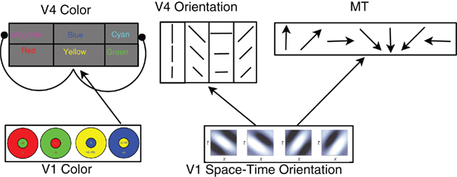
Figure 1. Architecture of the cortical model. In the V1 color layer, there are four color opponent (center+/surround−) responses corresponding to green+/red−, red+/green−, blue+/yellow−, and yellow+/blue−. The V4 color layers are composed of six color responses with both excitatory and inhibitory neurons for each color. For clarity, only the connections for Yellow are shown. V4 Yellow excitatory and inhibitory populations receive input from yellow center, blue surround cells in area V1 (normal arrow), and the V4 yellow inhibitory population inhibits the Magenta and Cyan excitatory groups (arrows with circular heads). The feed-forward connectivity is similar for Red, Green, and Blue. Cyan and Magenta receive feed-forward connections from two V1 layers: Green, Blue and Red, Blue (respectively). The V1 space–time orientation layer contains 28 space–time oriented filters at three spatial resolutions at each spatial location. These filters are converted into Poisson spike trains and project to MT and V4 Orientation neurons. See text for connectivity details.
The cortical model presented here not only showcases many of the simulator capabilities, but it also provides a starting point for computational neuroscientists to develop more complex simulations of cortical visual processing. The simulations below show examples of how to input images or videos into the model. Using the API described above, modelers can add more details to the current areas, such as the connectivity and cell classes found in layered neocortex, or add other areas. Moreover, the biologically inspired model of V1 motion selectivity, which has been optimized for GPUs, can be used with SNN or in other applications.
Cortical model of color selectivity
Using our simulator environment, we construct a model of color selectivity based on known V1 to V4 connectivity and the opponent-color theory (De Valois et al., 1958; Livingstone and Hubel, 1984). Following the opponent-color theory, we construct a rate-based model of area V1 where we have center-surround units that are selective to (1) red center, green surround; (2) green center, red surround; (3) yellow center, blue surround; and (4) blue center, yellow surround. The opponent receptive fields are made of 2-D Difference of Gaussians with a center SD of 1.2 pixels and a surround of 1.6 pixels. These 2-D Difference of Gaussians filters were then convolved with the input image. Color opponent signals are then converted to spike trains using Poisson spike generators (see Spike Generators specified above) and connected to populations that are selective to one of six colors: red, green, blue, yellow, magenta, and cyan. Each color has both an excitatory and inhibitory group, for a total of 12 V4 color groups. Each group in V1 and V4 has 1,024 (32 by 32) neurons.
Each population of V4 Red, Green, Blue, and Yellow V4 neurons receives input from the corresponding V1 color neurons (e.g., Red V4 receives input from Red V1). However, Magenta and Cyan, being secondary colors and not represented in area V1 were different; Magenta received equal input from both V1 Red and V1 Blue, whereas, Cyan received input from Green and Blue. All V4 receptive fields were 2-D Gaussian shaped from the V1 layers with a SD of 1.7 neurons (pixels). This feed-forward connectivity from the V1 layer to the V4 layer is shown in Figure 1. Each box represents both excitatory and inhibitory neurons for each color. The inhibitory population inhibits the excitatory populations (Figure 1, arrows with circular head). The inhibition causes responses to peak at their appropriate color. Without inhibition, the secondary colors (magenta, cyan, and yellow) would respond maximally to a broad range of colors and not have a peak at the desired spectral location.
The color selectivity profiles are shown in Figure 2, where the response of a single neuron is shown as a function of color input. The inputs were cycled between all combinations of RGB (Red–Green–Blue) values that summed to a constant value of 1, the far left corner corresponds to pure green, the far right is pure red, and the near corner is pure blue. The relative RBG values are converted to spike rates using a Poisson Spike Generator. The V4 responses shown in Figure 2 reveal that the neuronal units have selectivity to their preferred colors and the appropriate broad tuning to a range of hues (see Figure 2), and are similar to those found in macaque V4 (Kotake et al., 2009). For example, the panel labeled Red has highest firing rate for pure red, but responds to a lesser degree to purple and orange. The source code for this example can be found in the file titled “main_colorcycle.cpp” and the MATLAB script to analyze the results can be found in “colorcycle.m.”
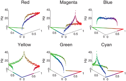
Figure 2. V4 color selectivity. Shown are responses of six excitatory V4 color units to a color stimulus cycling through all combinations of RGB (Red–Green–Blue) values that sum to a constant value of 1. The X- and Y-axes correspond to the color shown: the far left corner corresponds to pure green, the far right is pure red, and the near corner is pure blue. The Z axis represents the firing rate of the neuron in Hertz. One can clearly see that for example the Red unit (upper left tile) responds maximally to a pure red stimulus, and each unit responds maximally to its corresponding pure color.
To further demonstrate the performance of the V4 color model, we simulate the response of this network to color-blindness test images, shown in Figure 3. A standard colorblind test image was used that contained the number 6. The color content of this image was then modified so as to maximally activate different color populations (Figure 3 top row). In order to resolve the number 6 with sufficient resolution, we increased the input image size to 250 by 250 and adjusted the V4 populations accordingly. The firing rate responses of the six neural populations are shown in Figure 3 (Rows 2–7) as a gray scale image: black is no response and white is high response. The number “6” clearly “pops-out” in the network responses in nearly all of the configurations. The source code for this example can be found in the file titled “main_colorblind.cpp” and the MATLAB script to analyze the results can be found in “colorblind.m.”
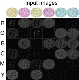
Figure 3. V4 responses to colorblind test images. Six versions of the same test image with the number 6 are used (top row). The color composition is varied so as to activate different color populations. The response of the six color regions (rows) to the six test images (columns) is shown in gray scale: no response is black and highest response is white. As one can see, under most configurations the number “6” pops-out in the neural responses.
Cortical model of motion and orientation selectivity
To generate motion selective responses, we used the Simoncelli and Heeger motion energy model for V1 (Simoncelli and Heeger, 1998). We re-implemented the motion energy model to run on the GPU. The code, (see “v1ColorME.cu” in the simulator source code directory), can be used as an efficient, standalone implementation of motion selectivity.
The Simoncelli and Heeger model uses an array of 28 space–time oriented filters (Third derivative of a Gaussian) at three spatial resolutions for a total of 84 filter responses. These filter responses are half rectified and squared to construct complex cell responses. The resulting complex cell responses are normalized by the response of all space–time orientations. Note that for the V1-complex cell normalization step, we normalize by the responses within a large Gaussian envelope instead of across the entire population as originally implemented by Simoncelli and Heeger. This was done to be more biologically realistic and has the effect of having spatially localized normalization instead of a single global normalization. These 84 complex filter responses can then be used to construct MT receptive fields that are selective to different directions and speeds of motion. The 84 rate-based responses were converted to Poisson spike trains using a Poisson spike generator (see Spike Generators above).
MT motion processing. The neurons in our MT model responded preferentially to one of eight different directions and three different speed preferences at a spatial location. The response of the MT neuron’s receptive field was based on connectivity from the V1 motion selective neurons. The connections from the 84 V1 units at a given pixel location to the MT neuron’s receptive field are quite complicated. Simply stated, the probability of a connection is proportional to the projection of the V1 cell’s receptive field onto a plane in the spatial frequency–temporal frequency domain. The slope of this plane defines the speed preference of the resulting MT cell and the rotation of the plane around the time axis defines the direction preference. For more information see Simoncelli and Heeger (1998).
To test the behavior of this model, we developed a paradigm equivalent to the random dot kinematogram (RDK) experiments performed with monkeys and humans (Roitman and Shadlen, 2002; Resulaj et al., 2009). We constructed a simple decision criterion, in which eight decision neurons (one for each of the eight directions of motion) sum all the MT responses selective to a direction of motion (see Figure 4; PFC). The decision rule was the first PFC neuron (corresponding to a direction) to spike 10 times signals a choice for that direction. The RDK stimulus was constructed out of 100 random dots on a 32 by 32 input movie. The motion in the stimulus was varied between 0 and 100% coherence and was one of two directions: left or right. Each stimulus frame was shown for 10 ms of simulation time and each coherence/direction configuration was shown for a total of 32 frames before another coherence and direction were chosen. For the RDK experiment we compared rightward responses to leftward responses and the results, which are shown in Figure 4, are comparable to human psychophysical experiments (Resulaj et al., 2009). The source code for this example can be found in the file titled “main_rdk.cpp” and the MATLAB script to analyze the results can be found in “rdk.m.”
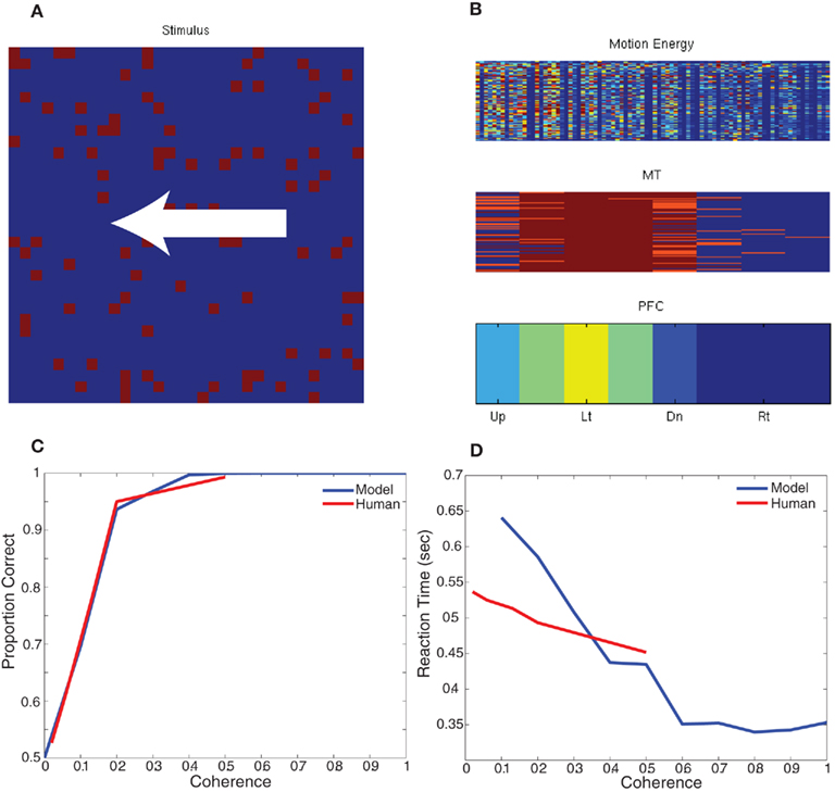
Figure 4. Simulation of Random Dot Kinematigram task (RDK). (A) The stimulus is composed of random moving dots. The coherence is varied between 0 and 100% and the direction of motion is either to the left or right. (B) The response of the network to an example stimulus. The firing rate of each unit is shown the heat of the color; blue is no response and red is high response. In the bottom of panel (B), the firing rate of the decision neurons (PFC) clearly show that the unit corresponding to leftward motion is responding maximally. (C,D) Comparison of the network response and human data for different levels of coherence dot movement. (C) Correct decision-making as a function of motion coherence. (D) Reaction time as a function of motion coherence. Human psychophysical data was adapted from (Resulaj et al., 2009).
V4 orientation. The motion energy responses can also be used to generate orientation selective responses. Since there are units in the 28 space–time filters that are more selective to orientation than motion, their responses can be used to generate a population of V4 orientation selective units. To qualitatively test the performance of the orientation selectivity, we constructed a simple stimulus composed of oriented gratings. We used four orientations and presented them to the network using a 32 by 32 resolution input image. The results show strong selectivity of V4 neurons to their preferred orientations (see Figure 5). Shown on the left hand side was the input image (four rows one for each orientation) and the corresponding response of the network is shown on the right hand side (four columns). Each column corresponds to a neural population selective to a different orientation. Each orientation has a total of 1,024 (32 by 32) neurons. The firing rate of each neuron is shown in pseudo-color; blue is no response and red is high response. The halos observed in many of the responses were due to edge effects of the motion energy filters. The source code for this example can be found in the file titled “main_orientation.cpp” and the MATLAB script to analyze the results can be found in “orientation.m.”
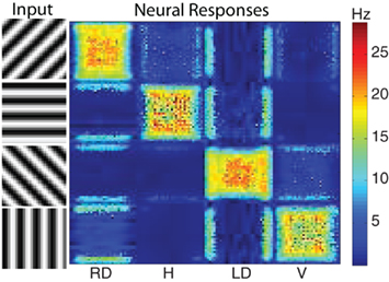
Figure 5. The response of the V4 orientation filters to different oriented stimuli. The four stimuli presented to the network are shown on the left. On the right are the neural responses of the four different orientation populations: right diagonal (RD), horizontal (H), left diagonal (LD), and vertical (V). Each population has 1024 neurons (32 by 32) and the firing rate of each neuron is shown in pseudo-color with blue being no response and red being high response. The corresponding firing rates are given by the color bar to the right of the neural populations. As one can see the strongest activity of each population corresponds to the stimuli corresponding to its preferred orientation.
Computational Performance
We measured the computational performance of both the randomly connected network, given in Section “Simple Source Code to Make a Randomly Connected Network Capable of Sustained Activity and Learning” in the Appendix, and the cortical model described in the previous section. GPU simulations were run on a NVIDA Tesla C1060 using CUDA, and CPU simulations were run on an Intel(R) Core(TM) i7 CPU 920 at 2.67 GHz.
For the randomly connected network, we ran simulations of various sized networks having a mixture of 80% excitatory and 20% inhibitory neurons. This allowed us to quantitatively compare the performances of GPU simulations to CPU simulations, and qualitatively compare the present simulation to our prior simulator (Nageswaran et al., 2009). The number of neurons in these simulations ranged from 1,000 to 300,000 neurons, plus an additional 10% of Poisson generator neurons. The Poisson spike generator neurons were used to drive the networks at an average firing rate of approximately 7 and 13 Hz. The synapses per neuron ranged from 100 to 500 connections. In the larger simulations, the GPU execution time was 12–18 times faster than the CPU at both firing rates (see Figures 6A,C). In our previous spiking neural network simulator, we reported that a random network with 100,000 neurons and a 100 connections per neuron was 1.5 times slower than real-time (Nageswaran et al., 2009). In the present simulator, networks with 110,000 neurons and 100 synaptic connections per neuron took roughly 2 s of clock time for every second of simulation time at both 7 and 13 Hz activity (see Figures 6B,D). More synapses per neuron incurred a computational cost at higher firings rates. For example, networks of 110 K neurons with 500 connections per neuron took 6 s of clock time per second of simulation time at 7 Hz activity and 10 s of clock time per second of simulation at 13 Hz activity (see Figures 6B,D). Some of the differences in performance between our previous simulator and the present one were due to the addition of conductance equations and the extra Poisson spiking neurons. In the prior simulator, which was current-based, spontaneous activity was achieved by simply injecting current generated spiking activity. In the present simulator, spiking activity is generated by Poisson generator input neurons. Despite the additional features and new programming interface, the present simulator is similar in performance to the earlier spiking network simulator.
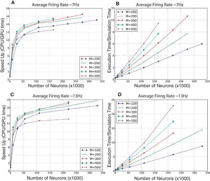
Figure 6. Evaluation of computational performance in randomly connected networks of 80% excitatory and 20% inhibitory neurons. An additional 10% of the neurons were Poisson spike generators that drove network activity. The number of neurons in the networks tested were 1,100, 11,000, 27,500, 55,000, 110,000, 220,000, and 330,000. M denotes the number of synapses per neuron. (A) Speedup, which is given as the ratio of CPU to GPU execution time, for networks with an average firing rate of 7 Hz. (B) Simulation speed, which is given as the ratio of GPU execution time over real-time, for networks with an average firing rate of 7 Hz. (C) Speedup, which is given as the ratio of CPU to GPU execution time, for networks with an average firing rate of 13 Hz. (D) Simulation speed, which is given as the ratio of GPU execution time over real-time, for networks with an average firing rate of 13 Hz.
We ran further performance metrics on the cortical model of color selectivity introduced in Section “Cortical Model of Color Selectivity” (see source code given in main_colorcycle.cpp) to quantitatively compare the performances of GPU simulations to CPU simulations. The network sizes ranged from 16 × 16 image frames (4,368 neurons) to 240 × 240 image frames (1,114,368 neurons). Note that the image height and width were increased by powers of two, except for the 240 × 240 network, which was the largest network that could be fit on the GPU card. The GPU simulations showed impressive performance gains over the CPU simulations, especially as the network size increased (see Figure 7A). The execution time of the cortical color model was slightly faster than real-time for the 32 × 32 image (69,696 neurons) network (see Figure 7B).
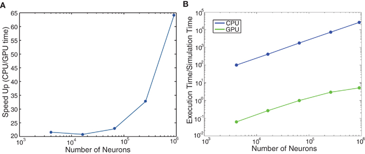
Figure 7. Evaluation of computational performance in the cortical model of color selectivity. The number of neurons in the networks tested were 4,368, 17,440, 69,696, 278,656, 979,440, and 1,114,368. (A) Speedup, which is given as the ratio of CPU to GPU execution time. (B) Simulation speed, which is given as the ratio of GPU execution time over real-time.
The complete model, which combined area MT, V4 color selectivity, and V4 orientation selectivity has 138,240 neurons and 29,547,000 synapses at a spatial resolution of 32 by 32. Running these 138 K neurons on a single NVIDIA C1060 GPU runs in approximately 0.95 of real-time; meaning it runs slightly faster than real-time. For the 64 by 64 input resolution, this network currently does not fit on a single GPU and as such required being run on the CPU which was approximately 36 times slower than real-time. The 64 by 64 network contains 552,960 neurons and 118,188,000 synapses.
Discussion
We have presented a simulation environment that supports the construction of large-scale models of SNN. The present paper serves two purposes: (1) Provide a simulation environment that can benefit the neuroscience community. To that end, we have given step-by-step instructions on how to construct networks of spiking neurons, and have made available the source code for running and analyzing these networks. (2) Present cortical models of visual processing that can be used for computational neuroscience experiments. The responses of neurons in the cortical visual processing model were comparable to electrophysiological results (De Valois et al., 1958; Livingstone and Hubel, 1984; Simoncelli and Heeger, 1998; Roitman and Shadlen, 2002), and the behavioral responses were in agreement with psychophysical data (Resulaj et al., 2009). The model can be readily expanded or parts may be extracted for specific computational models. For example, the efficient implementation of a V1 model of motion energy (Simoncelli and Heeger, 1998), which is rate-based, may be used as a standalone model in motion selectivity experiments.
The main features of the model are: (1) A flexible interface for creating neural networks. (2) Standard equations for the Izhikevich neuron (Izhikevich, 2004). This neuron model is very popular among the computational neuroscience community for being efficient, with only a few open parameters, yet supporting a wide-range of biophysically accurate dynamics. (3) Standard equations for AMPA, NMDA, and GABA conductances (Izhikevich et al., 2004). (4) Standard equations for STDP (Song et al., 2000). (5) Standard equations for STP (Markram et al., 1998; Mongillo et al., 2008). (6) An efficient implementation on either CPU or GPU environments.
The current implementation extends our previous work with new functionality, configurability, as well as eliminating some of the limitations of the previous implementation. Current GPU cards limit the size of the simulations due to memory constraints. To address these limitations, future work on GPU implementations will include: (1) interfacing our simulation environment with AER-based neuromorphic devices (Lichtsteiner et al., 2006), (2) exploiting new capabilities the GPU FERMI architecture, such as L2 cache, concurrent kernel execution, (3) and multi-GPU peer-to-peer communication (NVIDIA 2010). In the future, we plan to support more neuron models, such as integrate and fire models with adaptation (Jolivet et al., 2004; Brette and Gerstner, 2005; Gerstner and Naud, 2009; Kobayashi et al., 2009; Rossant et al., 2011), as well as other spike dependent plasticity rules (Van Rossum et al., 2000; Brader et al., 2007; Morrison et al., 2007; Urakubo et al., 2008). Given the modular code structure, we believe that these additions can be incorporated in such a way that users will be able to mix and match these models and learning rules as best fits their simulations. Furthermore, future versions of our simulator environment may take advantage of recent code generation tools such as NineML2, LEMS – Low Entropy Model Specification3, and the Brian simulator’s code generation package (Goodman, 2010) to facilitate the construction of simulations.
Our prior model, which was made available to the public, was an efficient implementation of the Izhikevich neuron on graphics processors (Nageswaran et al., 2009). This implementation was very popular among the research communities and demonstrated an interest in implementations that support large-scale modeling on generic computer platforms. The current implementation, which adds many important features, has only a slight performance penalty compared to our previous simulation and demonstrates efficient performance on both CPU and GPU platforms (see Figures 6 and 7). We hope the current implementation, which extends the functionality and usability of the original model, will find similar popularity.
Conflict of Interest Statement
The authors declare that the research was conducted in the absence of any commercial or financial relationships that could be construed as a potential conflict of interest.
Acknowledgments
This work was supported in part by the Defense Advanced Research Projects Agency (DARPA) subcontract 801888-BS.
Footnotes
References
Boahen, K. (2006). Neurogrid: emulating a million neurons in the cortex. Conf. Proc. IEEE Eng. Med. Biol. Soc. (Suppl.), 6702.
Bower, J. M., and Beeman, D. (2007). Constructing realistic neural simulations with GENESIS. Methods Mol. Biol. 401, 103–125.
Brader, J. M., Senn, W., and Fusi, S. (2007). Learning real-world stimuli in a neural network with spike-driven synaptic dynamics. Neural. Comput. 19, 2881–2912.
Brette, R., and Gerstner, W. (2005). Adaptive exponential integrate-and-fire model as an effective description of neuronal activity. J. Neurophysiol. 94, 3637–3642.
Brette, R., Rudolph, M., Carnevale, T., Hines, M., Beeman, D., Bower, J. M., Diesmann, M., Morrison, A., Goodman, P. H., Harris, F. C. Jr., Zirpe, M., Natschlager, T., Pecevski, D., Ermentrout, B., Djurfeldt, M., Lansner, A., Rochel, O., Vieville, T., Muller, E., Davison, A. P., El Boustani, S., and Destexhe, A. (2007). Simulation of networks of spiking neurons: a review of tools and strategies. J. Comput. Neurosci. 23, 349–398.
Davison, A. P., Bruderle, D., Eppler, J., Kremkow, J., Muller, E., Pecevski, D., Perrinet, L., and Yger, P. (2008). PyNN: a common interface for neuronal network simulators. Front. Neuroinform. 2:11.
De Valois, R. L., Smith, C. J., Kitai, S. T., and Karoly, A. J. (1958). Response of single cells in monkey lateral geniculate nucleus to monochromatic light. Science 127, 238–239.
Drewes, R., Zou, Q., and Goodman, P. H. (2009). Brainlab: a python toolkit to aid in the design, simulation, and analysis of spiking neural networks with the neocortical simulator. Front. Neuroinform. 3:16.
Fidjeland, A. K., and Shanahan, M. P. (2010). “Accelerated simulation of spiking neural networks using GPUs,” in Proceedings IEEE International Joint Conference on Neural Networks, Barcelona.
Goodman, D., and Brette, R. (2008). Brian: a simulator for spiking neural networks in python. Front. Neuroinform. 2:5.
Goodman, D. F. (2010). Code generation: a strategy for neural network simulators. Neuroinformatics 8, 183–196.
Hines, M. L., and Carnevale, N. T. (1997). The NEURON simulation environment. Neural. Comput. 9, 1179–1209.
Hines, M. L., and Carnevale, N. T. (2001). NEURON: a tool for neuroscientists. Neuroscientist 7, 123–135.
Izhikevich, E. M. (2004). Which model to use for cortical spiking neurons? IEEE Trans. Neural Netw. 15, 1063–1070.
Izhikevich, E. M., Gally, J. A., and Edelman, G. M. (2004). Spike-timing dynamics of neuronal groups. Cereb. Cortex 14, 933–944.
Jayet Bray, L. C., Quoy, M., Harris, F. C., and Goodman, P. H. (2010). A circuit-level model of hippocampal place field dynamics modulated by entorhinal grid and suppression-generating cells. Front. Neural Circuits 4:122.
Jolivet, R., Lewis, T. J., and Gerstner, W. (2004). Generalized integrate-and-fire models of neuronal activity approximate spike trains of a detailed model to a high degree of accuracy. J. Neurophysiol. 92, 959–976.
Kobayashi, R., Tsubo, Y., and Shinomoto, S. (2009). Made-to-order spiking neuron model equipped with a multi-timescale adaptive threshold. Front. Comput. Neurosci. 3:9.
Kotake, Y., Morimoto, H., Okazaki, Y., Fujita, I., and Tamura, H. (2009). Organization of color-selective neurons in macaque visual area V4. J. Neurophysiol. 102, 15–27.
Laughlin, S. B., and Sejnowski, T. J. (2003). Communication in neuronal networks. Science 301, 1870–1874.
Lichtsteiner, P., Posch, C., and Delbruck, T. (2006). A 128 × 128 120dB 30mW asynchronous vision sensor that responds to relative intensity change. IEEE Dig. Tech. Papers 508–509.
Livingstone, M. S., and Hubel, D. H. (1984). Anatomy and physiology of a color system in the primate visual cortex. J. Neurosci. 4, 309–356.
Markram, H., Wang, Y., and Tsodyks, M. (1998). Differential signaling via the same axon of neocortical pyramidal neurons. Proc. Natl. Acad. Sci. U.S.A. 95, 5323–5328.
Mongillo, G., Barak, O., and Tsodyks, M. (2008). Synaptic theory of working memory. Science 319, 1543–1546.
Morrison, A., Aertsen, A., and Diesmann, M. (2007). Spike-timing-dependent plasticity in balanced random networks. Neural. Comput. 19, 1437–1467.
Nageswaran, J. M., Dutt, N., Krichmar, J. L., Nicolau, A., and Veidenbaum, A. V. (2009). A configurable simulation environment for the efficient simulation of large-scale spiking neural networks on graphics processors. Neural. Netw. 22, 791–800.
Nageswaran, J. M., Richert, M., Dutt, N., and Krichmar, J. L. (2010). “Towards reverse engineering the brain: modeling abstractions and simulation frameworks,” in VLSI System on Chip Conference (VLSI-SoC), 2010 18th IEEE/IFIP, Madrid.
Navaridas, J., Luj, M., Miguel-Alonso, J., Plana, L. A., and Furber, S. (2009). “Understanding the interconnection network of SpiNNaker,” in Proceedings of the 23rd International Conference on Supercomputing. (Yorktown Heights, NY: ACM).
Rangan, V., Ghosh, A., Aparin, V., and Cauwenberghs, G. (2010). A subthreshold aVLSI implementation of the Izhikevich simple neuron model. Conf. Proc. IEEE Eng. Med. Biol. Soc. 2010, 4164–4167.
Resulaj, A., Kiani, R., Wolpert, D. M., and Shadlen, M. N. (2009). Changes of mind in decision-making. Nature 461, 263–266.
Roitman, J. D., and Shadlen, M. N. (2002). Response of neurons in the lateral intraparietal area during a combined visual discrimination reaction time task. J. Neurosci. 22, 9475–9489.
Rossant, C., Goodman, D. F., Fontaine, B., Platkiewicz, J., Magnusson, A. K., and Brette, R. (2011). Fitting neuron models to spike trains. Front. Neurosci. 5:9.
Simoncelli, E. P., and Heeger, D. J. (1998). A model of neuronal responses in visual area MT. Vision Res. 38, 743–761.
Song, S., Miller, K. D., and Abbott, L. F. (2000). Competitive Hebbian learning through spike-timing-dependent synaptic plasticity. Nat. Neurosci. 3, 919–926.
Urakubo, H., Honda, M., Froemke, R. C., and Kuroda, S. (2008). Requirement of an allosteric kinetics of NMDA receptors for spike timing-dependent plasticity. J. Neurosci. 28, 3310–3323.
Van Rossum, M. C., Bi, G. Q., and Turrigiano, G. G. (2000). Stable Hebbian learning from spike timing-dependent plasticity. J. Neurosci. 20, 8812–8821.
Vogels, T. P., and Abbott, L. F. (2005). Signal propagation and logic gating in networks of integrate-and-fire neurons. J. Neurosci. 25, 10786–10795.
Vogels, T. P., Rajan, K., and Abbott, L. F. (2005). Neural network dynamics. Annu. Rev. Neurosci. 28, 357–376.
Yudanov, D., Shaaban, M., Melton, R., and Reznik, L. (2010). “GPU-Based Simulation of Spiking Neural Networks with Real-Time Performance & High Accuracy,” in WCCI 2010 IEEE World Congress on Computational Intelligence, Barcelona.
Appendix
A MATLAB Function to Read the Spike Data Files
function s = readspikes(file, FrameDur)

if nargin<2

      FrameDur=1;

end

fid=fopen(file,’r’);

nrRead=1000000;

d2=zeros(0,nrRead);

s=0;

i=0;

while size(d2,2)==nrRead

      d2=fread(fid,[2 nrRead],’uint32’);

      d=d2;

      if isempty(d)

            if size(s,2) =max(d(2,:))+1 ||

size(s,1) =floor(d(1,end)/(FrameDur))+1,

s(floor(d(1,end)/(FrameDur))+1,max(d(2,:))+1)=0; end

s=s+full(sparse(floor(d(1,:)/(FrameDur))+1,d(2,:)+1,1,size(s,1),size(s,2)));

      end

      i=i+1;

end

fclose(fid);
A MATLAB Function to Read the Stored Network Files
function [groups, preIDs, postIDs, weights, delays, plastic, maxWeights] =

readNetwork (filename)

if ischar(filename)

      nid = fopen(filename,’r’);

else

      nid = filename;

end

version = fread(nid,1,’uint32’);

if version>1

      error([’Unknown version number ’ num2str(version)]);

end

nrGroups = fread(nid,1,’int32’);

groups = struct(’name’,{},’startN’,{},’endN’,{});

for g=1:nrGroups

      groups(g).startN = fread(nid,1,’int32’)+1;

        groups(g).endN = fread(nid,1,’int32’)+1;

      groups(g).name = char(fread(nid,100,’int8’)’);

      groups(g).name = groups(g).name(groups(g).name>0);

end

nrCells = fread(nid,1,’int32’);

weightData = cell(nrCells,1);

nrSynTot = 0;

for i=1:nrCells

      nrSyn = fread(nid,1,’int32’);

      nrSynTot = nrSynTot + nrSyn;

      if nrSyn>0

            weightData{i} = fread(nid,[18 nrSyn],’uint8=>uint8’);

      end

end

if ischar(filename)

   fclose(nid);

end

alldata = cat(2,weightData{:});

weightData = {};

preIDs = typecast(reshape(alldata(1:4,:),[],1),’uint32’);

postIDs = typecast(reshape(alldata(5:8,:),[],1),’uint32’);

weights = typecast(reshape(alldata(9:12,:),[],1),’single’);

maxWeights = typecast(reshape(alldata(13:16,:),[],1),’single’);

delays = alldata(17,:);

plastic = alldata(18,:);
Simple source code to make a randomly connected network capable of sustained activity and learning
         #include “snn.h”


#define N 1000


int main()

{

   // create a network

   CpuSNN s(“global”);


   int g1=s.createGroup(“excit”, N*0.8, EXCITATORY_NEURON);

   s.setNeuronParameters(g1, 0.02f, 0.2f, -65.0f, 8.0f);


   int g2=s.createGroup(“inhib”, N*0.2, INHIBITORY_NEURON);

   s.setNeuronParameters(g2, 0.1f, 0.2f, -65.0f, 2.0f);


   int gin=s.createSpikeGeneratorGroup(“input”,N*0.1,EXCITATORY_NEURON);

   // make random connections with 10% probability

   s.connect(g2,g1,“

            random”, -1.0f/100, -1.0f/100, 0.1f, 1, 1, SYN_FIXED);

   // make random connections with 10% probability,

         // and random delays between 1 and 20

   s.connect(g1,g2,“

            random”,0.25f/100,0.5f/100,0.1f,1,20,SYN_PLASTIC);

   s.connect(g1,g1,“

            random”,6.0f/100,10.0f/100,0.1f,1,20,SYN_PLASTIC);


   // 5% probability of connection

   s.connect(gin,g1,“

            random”,100.0f/100,100.0f/100,0.05f,1,20,SYN_FIXED);


   float COND_tAMPA=5.0, COND_tNMDA=150.0;

   float COND_tGABAa=6.0, COND_tGABAb=150.0;

   s.setConductances(ALL,true,COND_tAMPA,COND_tNMDA,

                          COND_tGABAa,COND_tGABAb);


   // here we define and set the properties of the STDP.

         float ALPHA_LTP = 0.10f/100, TAU_LTP = 20.0f;

   float ALPHA_LTD = 0.12f/100, TAU_LTD = 20.0f;

   s.setSTDP(g1, true, ALPHA_LTP, TAU_LTP, ALPHA_LTD, TAU_LTD);


   // log every 10 sec, at level 1 and output to stdout.

   s.setLogCycle(10, 1, stdout);


   // put spike times into spikes.dat

   s.setSpikeMonitor(g1,"spikes.dat");


   // Show basic statistics about g2

   s.setSpikeMonitor(g2);


   //setup some baseline input

   PoissonRate in(N*0.1);

   for (int i=0;i<N*0.1;i++) in.rates[i] = 1;

   s.setSpikeRate(gin,&in);

   //run for 10 seconds

   for(int i=0; i < 10; i++) {


      // run the established network for a duration of 1 (sec)

         // and 0 (millisecond), in CPU_MODE

      s.runNetwork(1, 0, CPU_MODE);

   }


   FILE* nid = fopen(“network.dat”,“wb”);

   sim.writeNetwork(nid);

   fclose(nid);


   // display the details of the current simulation run

   s.printSimSummary();

   return 0;

}
Keywords: visual cortex, spiking neurons, STDP, short-term plasticity, simulation, computational neuroscience, software, GPU
Citation: Richert M, Nageswaran JM, Dutt N and Krichmar JL (2011) An efficient simulation environment for modeling large-scale cortical processing. Front. Neuroinform. 5:19. doi: 10.3389/fninf.2011.00019
Received: 14 May 2011; Accepted: 27 August 2011;
Published online: 14 September 2011.
Edited by:
Andrew P. Davison, CNRS, FranceReviewed by:
Eilif Muller, École Polytechnique Fédérale de Lausanne, SwitzerlandRomain Brette, École Normale Supérieure de Paris, France
Andreas Kirkeby Fidjeland, Imperial College London, UK
Copyright: © 2011 Richert, Nageswaran, Dutt and Krichmar. This is an open-access article subject to a non-exclusive license between the authors and Frontiers Media SA, which permits use, distribution and reproduction in other forums, provided the original authors and source are credited and other Frontiers conditions are complied with.
*Correspondence: Jeffrey L. Krichmar, Department of Cognitive Sciences, University of California, 2328 Social and Behavioral Sciences Gateway, Irvine, CA 92697-5100, USA. e-mail: jkrichma@uci.edu